Publisher’s version / Version de l'éditeur:
ASHRAE Transactions, 111, 2, pp. 583-594, 2005-05-01
READ THESE TERMS AND CONDITIONS CAREFULLY BEFORE USING THIS WEBSITE.
https://nrc-publications.canada.ca/eng/copyright
Vous avez des questions? Nous pouvons vous aider. Pour communiquer directement avec un auteur, consultez la
première page de la revue dans laquelle son article a été publié afin de trouver ses coordonnées. Si vous n’arrivez pas à les repérer, communiquez avec nous à [email protected].
Questions? Contact the NRC Publications Archive team at
[email protected]. If you wish to email the authors directly, please see the first page of the publication for their contact information.
NRC Publications Archive
Archives des publications du CNRC
This publication could be one of several versions: author’s original, accepted manuscript or the publisher’s version. / La version de cette publication peut être l’une des suivantes : la version prépublication de l’auteur, la version acceptée du manuscrit ou la version de l’éditeur.
Access and use of this website and the material on it are subject to the Terms and Conditions set forth at
Guidelines for the use of CFD simulations for fire and smoke modeling
Hadjisophocleous, G. V.; McCartney, C. J.
https://publications-cnrc.canada.ca/fra/droits
L’accès à ce site Web et l’utilisation de son contenu sont assujettis aux conditions présentées dans le site LISEZ CES CONDITIONS ATTENTIVEMENT AVANT D’UTILISER CE SITE WEB.
NRC Publications Record / Notice d'Archives des publications de CNRC: https://nrc-publications.canada.ca/eng/view/object/?id=d509267a-b845-42ad-877d-52d5fd06ec41 https://publications-cnrc.canada.ca/fra/voir/objet/?id=d509267a-b845-42ad-877d-52d5fd06ec41
http://irc.nrc-cnrc.gc.ca
G u i d e l i n e s f o r t h e u s e o f C F D s i m u l a t i o n s f o r
f i r e a n d s m o k e m o d e l i n g
N R C C - 4 7 7 4 0
H a d j i s o p h o c l e o u s , G . V . ; M c C a r t n e y , C . J .
A version of this document is published in / Une version de ce document se trouve dans: ASHRAE Transactions, v. 111, no. 2, 2005, pp. 583-594
The material in this document is covered by the provisions of the Copyright Act, by Canadian laws, policies, regulations and international agreements. Such provisions serve to identify the information source and, in specific instances, to prohibit reproduction of materials without written permission. For more information visit http://laws.justice.gc.ca/en/showtdm/cs/C-42
Les renseignements dans ce document sont protégés par la Loi sur le droit d'auteur, par les lois, les politiques et les règlements du Canada et des accords internationaux. Ces dispositions permettent d'identifier la source de l'information et, dans certains cas, d'interdire la copie de documents sans permission écrite. Pour obtenir de plus amples renseignements : http://lois.justice.gc.ca/fr/showtdm/cs/C-42
Guidelines for the Use of CFD Simulations for Fire and Smoke Modeling
G. V. Hadjisophocleous, Ph.D.,
Department of Civil and Environmental Engineering, Carleton University 1125 Colonel By Drive, Ottawa, Ontario, K1S 5B6, Canada
C. J. McCartney
Fire Research Program, Institute for Research in Construction National Research Council Canada
Bldg M-59 Montreal Road, Ottawa, K1A 0R6, Canada
Abstract
This paper presents a 'back to basics' examination of CFD techniques as they relate to the modelling of fire development and smoke production. The paper aims at providing a better understanding of fundamental fire dynamics concepts, their limitations and impact on model predictions. Key issues examined include: grid resolution, plume entrainment rates, combustion models, smoke modeling, radiative fraction, non-orthogonal
geometries, interface height calculation, and boundary layer modeling. Guidelines for the proper treatment of each issue are given as well as advice on avoiding common pitfalls. The NIST's Fire Dynamics Simulator (FDS) software is discussed in detail, however many of the issues, results and discussions are applicable to other CFD models. The fire scenarios considered deal with fires in compartments and atria due to their relevance to ASHRAE members. Where appropriate, comparative results based on the sample models provided with FDS are presented.
INTRODUCTION
The use of Computational Fluid Dynamics (CFD) models, or field models, in the design of smoke management and smoke control systems for large and geometrically complex spaces such as atria and subway stations, as well as underground tunnels, is becoming more common as a result of increased computer speeds at lower costs and the
availability of CFD models. There are many examples in the literature where the results of CFD models were the basis of smoke control and smoke management system
designs [1,2]. This trend, however, has raised the concern by many, in both the authorities and the engineering groups that some of the users may not have a full appreciation of the complexities of CFD models and the impact on the solution of a number of parameters used in modelling fires and smoke movement. As a result of the increased user-friendliness of CFD models, it is now possible for users who have a minimal knowledge of the theories behind CFD models to use them and produce results that look reasonable and defendable. One such parameter, discussed in some detail by Yau et al. [3], is the treatment of the fire source in CFD models. The authors have demonstrated that it may be possible to use a volumetric heat source to describe the fire instead of a combustion model and obtain good results provided that certain rules are followed. The authors present guidance in selecting the area and the volume of the fire to ensure good results. This type of guidance is also required for a number of other parameters used in setting up CFD models to perform such simulations.
The objective of this paper is to provide some guidance to users of CFD models on some of the important parameters that affect the predicted results. This paper is not intended as an introduction to CFD techniques or their application. The paper presents
results of investigations and comparisons with accepted correlations that demonstrate how these parameters influence the results and show what is required to ensure that these parameters have values that ensure accuracy with minimum run times.
Parameters considered in this study are grid resolution, plume entrainment rates, combustion models, radiative fraction, non-orthogonal geometries, interface height calculation, and boundary layer modeling. Results presented in this paper are useful to fire protection professionals who design fire safety systems in buildings using CFD models and to authorities who review these designs.
METHODOLOGY
The application of CFD models to any problem involves a number of basic steps. These steps are the following:
• Computational domain: The computational domain defines the volume over which the solution will be obtained. For some problems the computational domain is obvious, however for others, such as for example where door or window plumes are expected definition of the computational domain should be carefully selected to ensure accurate predictions.
• Grid generation: a grid to cover the computational domain is constructed in such a way to ensure that a grid-independent solution is obtained. The higher the number of grid points the longer the computational time will be, hence it is essential to generate grids that provide accurate and affordable solutions. Grid properties such as aspect ratio may have an impact on the solution and should be carefully
examined during the preliminary runs.
• Boundary conditions: at each boundary of the computational domain it is necessary to define thermal and hydrostatic boundary conditions. In the case of free flows the boundary conditions should be defined away from the flow so that they do not influence the solution.
• Fire modelling: modelling the fire can be done by assigning a volumetric heat source at the control volumes where combustion takes place or by using a combustion model. Care should be taken in defining volumetric heat sources so that realistic plume characteristics are predicted.
To demonstrate the impact of the above on the predictions, in this work, the CFD model FDS developed by NIST [4,5] is used to simulate a number of scenarios. The scenarios were selected to allow an examination of the impact of model parameters on the
solution. The model results are then analysed and graphs are produced that clearly show this impact. Where possible the results of the model are compared with existing correlations.
GRID RESOLUTION
The use of smaller mesh elements in a CFD simulation generally increases the accuracy of the results. Spatial gradients are approximated using more points and, for large-eddy simulations, a greater proportion of the flow vortices are modelled directly without resorting to a turbulence model. The drawback of higher resolution meshes is their increased computational cost. A mesh resolution should be chosen which yields results with the desired accuracy but also takes into account limitations on available time and computational resources.
For CFD simulations of fire scenarios, mesh refinement is most important in the combustion volumes, plume boundaries and thermal layer interfaces. Combustion models require fine enough mesh resolutions to accurately model the production of heat and fire products. Plume boundaries and layer interfaces represent areas of relatively high gradients in the flow and require small mesh elements to accurately predict entrainment and mixing rates.
Grid resolution also affects the accuracy of the mixture fraction model used in FDS. The use of coarse mesh elements in the combustion volume can lead to under predicted heat release rates and flame heights [5]. FDS makes some adjustments to the mixture fraction model to compensate for these effects. In contrast, grid resolution has little effect on the accuracy of volumetric heat source modeling. However, volumetric heat sources are characteristically poor at predicting flame heights.
The simulations presented for this issue are variations of the ‘plume3’ model supplied with FDS Version 3 [4]. A 0.2 m square burner is located in the center of a flow domain 1.6 m wide by 1.6 m deep by 3.6 m high (Figure 1). Three different mesh element sizes are used for a 24 kW fire and three heat release rates are used for the smallest mesh element size of 0.025 m (Table 1). The main comparison parameters are the vertical mass flow rate and plume centreline temperature profiles.
(Figure)
Figure 1. Geometry for ‘plume3’ simulations.
Table 1. Parameters for ‘plume3’ simulations.
Simulation Number of Mesh Elements Mesh Element Size (m) HRR1 (kW) HRRPUA2 (kW/m2) z03 (m) Theo. Flame Height (m) plume3_A 16,16,36 0.1 24 600 0.0657 0.608 plume3_B 32,32,72 0.05 24 600 0.0657 0.608 plume3_C 64,64,144 0.025 24 600 0.0657 0.608 plume3_D 64,64,144 0.025 48 1200 0.160 0.875 plume3_E 64,64,144 0.025 12 300 -0.00595 0.405
1. Heat release rate
2. Heat release rate per unit area 3. Virtual origin
The virtual origin is the elevation where an equivalent point source produces the same plume as a fire over an actual area. This parameter is used extensively in the analysis of fire plume dynamics and is calculated as:
z0 = -1.02 D + 0.083 Q2/5 (1)
where Q is the total heat release rate in kilowatts and D is the burner diameter in metres [6]. The area of the 0.2 m square burner in all models is 0.04 m2 and the grid is selected
to match the burner perimeter exactly. The equivalent diameter of the square burner is calculated as:
D = (4A/ π)1/2 = 0.2257 m (2)
The theoretical flame height, L, is calculated assuming normal atmospheric conditions [6]:
L = -1.02D + 0.235Q2/5 (3)
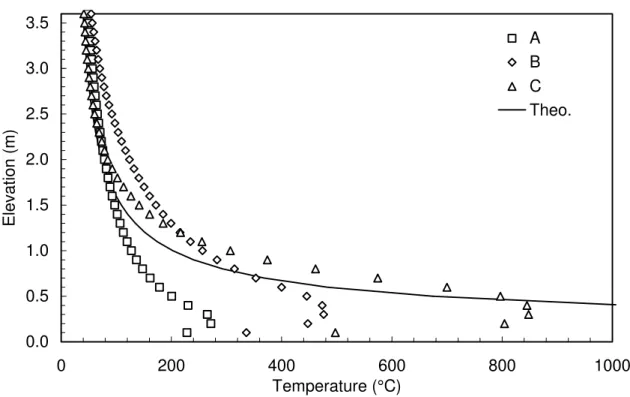
Figure 2 compares the plume centreline temperature predictions of simulations A through C as a function of height (z) with the following correlation:
T0 = 9.1 (T∞ / g cp2 ρ∞2)1/3 Qc2/3 (z-z0)-5/3 + T∞ (4)
where ρ∞, cp and T∞ are the density (kg/m3), heat capacity (kJ/kg-K) and temperature (K)
of the ambient air and Qc is the convective portion of the fire’s heat release rate (kW) [6].
The mass flow rate profiles for the 24 kW simulations with different mesh resolutions were also compared with the theoretical correlation based on the weak plume equations for axisymmetric plumes [6]:
m = 0.153 (g ρ∞2/cp T∞)1/3 Qc1/3 (z-z0)5/3 (5)
Equations 4 and 5 are experimental correlations and are therefore considered an accurate basis for comparison of numerical modeling results. Note that although these correlations were developed for axisymmetric fires, they are still relatively accurate for square fire sources.
Figure 2 compares the plume centreline temperature profiles for simulations A, B and C with the theoretical profile. Simulations A and B show significant deviations from the theoretical temperature profile. This is an indication that plume entrainment rates are being inaccurately modeled at these mesh resolutions. Simulation C gives a much better approximation to the theoretical centreline temperature profile.
(Figure)
Figure 2. Comparison of centreline temperature profiles for ‘plume3’ simulations.
Figure 3 compares the mass flow rate for simulations C, D and E with the theoretical profile. These results show that, for a constant mesh element size, the accuracy of the simulated profiles decreases with increasing fire size. This is consistent with Quintere and Ma’s guidelines that suggest the accuracy of plume modelling is dependant upon the non-dimensional fire size, Q*:
Q* = Q / (ρ∞cpT∞D2 (gD)1/2) (6)
All three simulated profiles show a divergence near the top of the flow domain. This is attributed to the effect of the open boundary condition propagating into the flow domain.
Figure 3. Comparison of ‘plume3’ mass flow rate profiles, various fire sizes.
Although the fires used here are much smaller than typical design fires for construction applications, the importance of grid resolution is still relevant. The non-dimensional fire size, Q*, may be used as a parameter for comparing grid resolutions for fires with different heat release rates. Quintiere and Ma [7] discuss this parameter in more detail.
ATRIUM PLUME RESOLUTION
Modeling of fire plume dynamics is a basic requirement for many fire protection engineering designs. Analysis of simple plumes can be performed using standard correlations. CFD techniques allow analysis of plumes with non-standard shapes or those plumes which interact with complex geometries. The main modeling issue is the mesh resolution required to accurately predict plume dynamics.
Most plume analyses require an estimate of the entrainment rate. This in turn affects plume size, temperature, mass flow rate and the depth of the hot layer formed in any enclosing volume. Accurate prediction of entrainment at the plume edges requires modeling of eddies down to a certain minimum size. For a large eddy simulation (LES) model such as that available in FDS, this requirement translates into a minimum mesh element size since any eddy smaller than this size will be estimated rather than modeled directly.
The simulations presented here are of a simple fire in an atrium. The atrium is 20 m square and 30 m high with no walls and a ceiling. No smoke exhaust ventilation is specified. A 4 MW fire, spread over 9 m2 is centered on the atrium floor. Two meshes are used for simulation D to allow higher resolution of the combustion volume: Mesh 1 is defined as a 6 m cube around the fire with open sides and top; Mesh 2 is defined as the remainder of the atrium and is modeled as a 20 m square by 24 m high volume. The remaining simulations use a single mesh over the entire atrium. All mesh elements are isometric and all simulations are solved to steady-state conditions. The main
parameters for comparison are the vertical mass flow rate and plume centreline temperature profiles.
(Figure)
Figure 4. Geometry for ‘atrium’ simulations.
Table 2. Parameters for ‘atrium’ simulations.
Simulation Mesh element size (m)
Solution time (h) atrium_D 0.1 (Mesh 1), 0.5 (Mesh 2) 98.2
atrium_E 0.5 2.84 atrium_F 0.25 18.8 atrium_G 0.2 41.4
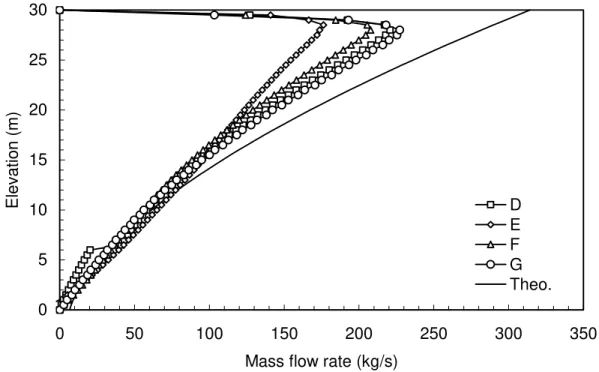
Figure 5 compares the mass flow rate profiles for all four simulations with the theoretical profile based on Equation 4. The results from simulation D are relatively close to the theoretical mass flow rate profile and are the closest of the four for the theoretical plume
centreline temperature profile. This is to be expected as simulation D has the highest resolution of the combustion volume. Higher resolution of the combustion volume improves the accuracy of the results at higher elevations compared to the 0.5 m single mesh in simulation E. However, there are noticeable discontinuities in both of the profiles from simulation D at the interface between the two meshes (z = 6.0 m). This is attributed to the sudden change in mesh size and may result in unknown modeling errors.
(Figure)
Figure 5. Comparison of mass flow rate profiles for ‘atrium’ simulations.
Of the three simulations using a single mesh, simulation G yields the profiles closest to the theoretical due to its high mesh resolution. Note that the discrepancy between results from simulation F (0.25 m) and G (0.2 m) show that 0.2 m is not a grid-insensitive resolution for this model. Additional modeling at higher mesh resolutions would be required.
The results from the ‘atrium’ simulations show that high resolution modelling of the combustion volume may not be necessary for accurate prediction of the bulk plume flow at higher elevations. This can result in computational savings, although selected grid sensitivity studies should be performed to verify the model’s accuracy. As a rough guideline, mesh resolutions in the order of 10-1 m should be used for plume models. Ma and Quintiere have recently published a mesh sensitivity study applied to plume
dynamics modeling [7].
ASPECT RATIO
The use of a non-isometric mesh to reduce the number of elements in a flow domain can significantly decrease solution times. Non-isometric elements are especially appropriate where there is a strong directed flow in the direction of the element transformation. The higher advection tends to decrease spatial gradients in the direction of flow, reducing the need for fine mesh elements along one axis. However, highly non-isometric mesh elements may introduce numerical errors into the simulation and affect the accuracy of the results.
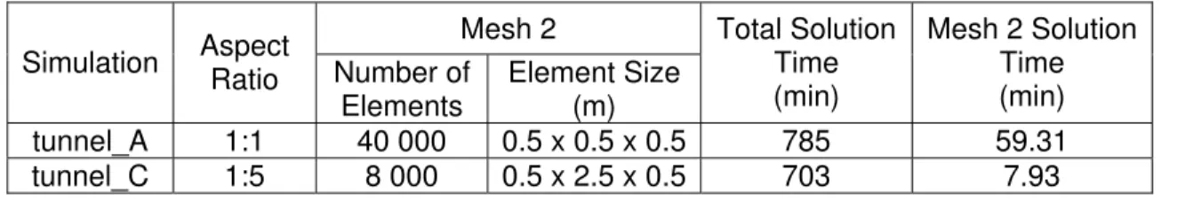
The simulations presented here are of a 60 m long, 10 m square tunnel open at one end with a 5 MW fire covering 9 m2 near the closed end. The burner is resolved with a 10 m cubic mesh (Mesh 1) using a relatively fine resolution of 0.25 m to accurately model the combustion process and plume dynamics. The remainder of the tunnel (Mesh 2) is resolved at 0.5 m along the tunnel width and height, and four different aspect ratios along the tunnel length: 1:1 (0.5 m), 1:5 (2.5 m) and 1:10 (5.0 m) (Table 3).
Table 3. Parameters for ‘tunnel’ simulations.
Mesh 2 Simulation Aspect Ratio Number of Elements Element Size (m) Total Solution Time (min) Mesh 2 Solution Time (min) tunnel_A 1:1 40 000 0.5 x 0.5 x 0.5 785 59.31 tunnel_C 1:5 8 000 0.5 x 2.5 x 0.5 703 7.93
tunnel_D 1:10 4 000 0.5 x 5.0 x 0.5 683 3.98
Table 3 also lists the solution times for the three simulations. The total solution time decreases as the number of elements in Mesh 2 is reduced.
The mass flow rate profiles along the tunnel were compared for all three simulations but are not presented here. This is an indicator of how well entrainment into the hot layer is modeled as it flows along the tunnel. Although the profile for simulation A may not be grid-insensitive, it still serves as a basis for comparison for the other two profiles. The profiles from simulations C and D both show a large increase in the mass flow rate along the middle portion of the tunnel, indicating larger entrainment rates into the hot layer. Both profiles also show a high amount of unstable variation near the end of the tunnel due to the propagation of the open boundary condition into the flow domain. This effect increases with the aspect ratio, carrying the variation farther into the flow domain.
Figure 6 compares the temperature profiles at the tunnel exit for all three simulations. This data supports the conclusion that increased aspect ratios artificially increase entrainment rates into the hot layer, leading to a thicker layer with lower temperature rise. From a design standpoint, this will affect the specification of tunnel heat detectors and, more importantly, increase estimates of the smoke exhaust system capacity.
(Figure)
Figure 6. Tunnel exit temperature profiles for ‘tunnel’ simulations.
The results of these simulations show that, although non-isometric mesh elements allow for savings in solution time, they should be applied carefully with selected comparison against results using smaller aspect ratios.
DOORWAY JET PLUMES
Compartment fires are of interest to many fire engineering professionals. Accurate modeling of compartment fire dynamics is critical in predicting such parameters as time to flashover, secondary ignition of objects, and smoke and heat production from the compartment. One issue affecting the accuracy of compartment fire simulations is the modeling of the doorway jet plume.
The doorway jet plume impacts conditions within the compartment through radiation heat transfer and interaction with the flow of combustion air into the compartment. It is
desirable to minimize the size of the flow domain in order to reduce computation time. However, if the plume is not modelled for a sufficient distance beyond the door, radiation will be lost from the flow domain and interaction with the combustion air layer will be poorly predicted. Therefore, a key modeling issue is how far outside the compartment opening the doorway plume should be modelled to achieve accurate results.
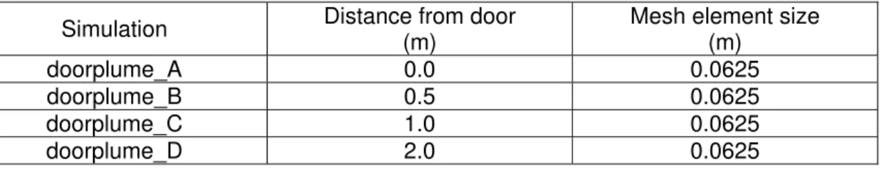
The simulations presented here are of simple compartment fires with different distances outside the room being included in the flow domain. The compartment is 2.5 m wide by 3.0 m long by 2.5 m high with a 1.5 m wide by 2.0 m high doorway centered in one of the shorter walls (Figure 7). A 1 m2, 500 kW burner is located at floor level centered against the wall opposite the doorway. Four different distances outside the room are included in the flow domain: 0.0, 0.5, 1.0, and 2.0 m (Table 4). A mesh element size of 0.0625 m is
used in all simulations. The simulations are run for 5 min to achieve steady-state conditions.
(Figure)
Figure 7. Geometry for ‘door-plume’ simulations.
Table 4. Parameters for ‘door-plume’ simulations.
Simulation Distance from door (m)
Mesh element size (m)
doorplume_A 0.0 0.0625
doorplume_B 0.5 0.0625
doorplume_C 1.0 0.0625
doorplume_D 2.0 0.0625
Temperature profiles were compared throughout the compartment. Figure 8 compares the door centreline temperature profiles for all four simulations. Results from simulation A are markedly different from the rest, with a higher flame temperature and increased hot layer elevations in the room and at the doorway opening. This is partly due to poor modeling of the complex flow dynamics at the doorway opening. The specification of an open flow domain boundary at the doorway changes the flow pattern across the door in order to satisfy the boundary conditions. The loss of radiation from the doorway jet plume back into the compartment may also be affecting the compartment temperature profiles.
Comparison of profiles B, C and D show little change in the temperature profiles as the modeled plume length is increased from 0.5 to 2.0 m beyond the door. This indicates that grid-insensitive results may be obtained even if only a short length of the doorway jet plume is modeled.
(Figure)
Figure 8. Door centerline temperature profiles for ‘door-plume’ simulations.
NON-ORTHOGONAL GEOMETRY
Although most commercial CFD software programs allow non-orthogonal geometries, FDS does not in order to increase solution efficiency. Orthogonal geometries are sufficient for a large number of CFD problems encountered by ventilation and fire protection engineering professionals. However, as a limited solution to non-orthogonal geometries, FDS allows the vorticity to be set to zero at the corners of obstructions. This prevents the formation of vortices that would not be present in the real flow, reducing errors due to increased entrainment and drag.
The simulations presented here show the effect of non-orthogonal geometries in FDS with and without vorticity compensation. The ‘tunnel’ model presented earlier is used as a basis for the ‘slope’ simulations. The tunnel is sloped at approximately 5° and both ends of the tunnel are specified as open boundary conditions (Figure 9). Simulation A models the sloped tunnel with a series of stair stepped obstructions. Simulation B uses
the same geometry but specifies the vorticity to be set to zero at the corners of the obstructions. Simulation C is a non-sloped tunnel for comparison purposes. Simulation D models the sloped tunnel as an orthogonal volume with the gravity vector specified approximately 5° from the vertical. All simulations use a single mesh with an element size of 0.5 m. The main parameters of interest are the mass flow rate profiles along the tunnels and the temperature profiles at the tunnel exit.
(Figure)
Figure 9. Geometry for ‘slope’ simulations.
Figure 10 compares the mass flow rate profiles along the tunnel for all four simulations. The mass flow rate predicted by simulation C is drastically lower than the rest because of the lack of slope. The increased buoyancy force in a sloped tunnel increases the flow rate of the hot layer along its entire length. The profile for simulation B is higher than either A or D. The absence of vorticity produced at the obstruction corners in simulation B reduces the amount of entrainment into the hot layer. This allows the hot layer to flow at a higher speed, increasing its mass flow rate. Simulations A and D have very similar profiles, showing that the use of a non-orthogonal gravity vector may only increase the mass flow rate slightly. It may be expected that the profile from simulation D should match the profile from simulation B more closely since both represent a flow with no increased vorticity generation. However, these simulations may be difficult to compare directly since their geometries are dissimilar.
(Figure)
Figure 10. Mass flow rate profiles for ‘slope’ simulations.
The temperature profiles at the tunnel exit were compared for simulations A and B but are not presented here. The hot layer temperature in simulation B is slightly lower, supporting the conclusion that entrainment into the hot layer is artificially increased by the obstruction corner vortices. Hot layer temperatures are of primary importance for tunnel smoke control as they affect the tendency of smoke to flow against the desired direction via back layering.
The results of these simulations show that vorticity compensation in FDS does make a difference in the flow dynamics around orthogonal geometries. The use of a non-orthogonal gravity vector may also be appropriate for simple geometries.
RADIATIVE FRACTION
Radiative fraction is the portion of a fire’s energy which is emitted as radiation to the surroundings. Radiative heat transfer strongly affects the development of flashover conditions, secondary ignition of materials, and hot layer depth and temperature. Accurate modeling of radiative heat transfer is essential for the majority of fire growth simulations.
Numerical modeling of radiation can be computationally expensive. Ideally, radiation transfer should be calculated over a large number of very small angles and over the entire spectrum of electromagnetic energy. Most practical simulations are limited in both respects due to the high computational costs. FDS uses a finite volume method to
calculate radiation transfer over a discrete number of angles. Options are available to use more angles, thus improving accuracy, or to use a six-band radiation model instead of the default grey-gas model. The default radiation model is stated to require about 20% of the total computational time [5]. Although radiative fraction in real fires varies with fuel type, temperature, available oxygen and soot concentration in the flame, FDS uses a constant value for radiative fraction.
The ‘roomfire3’ model provided with FDS is used to show the effect of radiative fraction on compartment fire dynamics. Three simulations were performed: one with the default radiative fraction of 0.35 and two with specified radiative fractions of 0.50 and 0.20. The default grey-gas radiation model is used with the default number of angles. The main comparison variable is the time to flashover.
Flashover with the default radiative fraction of 0.35 occurred at approximately 280 s. A radiative fraction of 0.50 caused this time to decrease to 165 s, and a radiative fraction of 0.20 prevented the room from reaching a flashover condition. The radiative fraction affects the time to flashover through the ignition of secondary objects in the room. Higher values cause these items to ignite more quickly, leading to flashover conditions much earlier, while lower values do not allow the secondary objects to ignite.
MATERIAL COMBUSTION PROPERTIES
Most real fire sources are composed of multiple materials with different combustion properties. Although extensive fire behaviour data is available for most materials, similar data for composite combinations of these materials is more limited. Fire protection engineering professionals have traditionally resorted to testing specific fuel packages in set scenarios to obtain data for input into numerical models. This case-by-case
approach can be both expensive and time-consuming.
FDS allows direct modeling of material combustion through two sets of material properties: chemical reaction stoichiometry properties and material combustion properties. Stoichiometry properties specify yields of fire products such as carbon monoxide and soot, and energy produced per unit of oxygen consumed. Combustion properties specify variables such as heat of combustion, density, thermal properties, ignition temperature and maximum burning rate. FDS continues to extend its basic capabilities to include more complex phenomena such as temperature dependant material properties and the formation of char.
Numerical modeling of complex fire sources poses some challenges. Direct modeling of the geometry and composition of a complex source may require an unreasonably high resolution mesh around the fire source. The simplest approximation is to replace the complex fire source with a single block whose material properties are an equivalent combination of the original materials. The method used to combine material properties is an important issue since it will affect both the fire development and generation of fire products.
The ‘blocks’ simulations presented here model a cone calorimeter test. A 100 mm square block 25 mm in height is placed under a radiant source. The source is removed after 60 s to allow free combustion. Four simulations were performed using two
materials typically found in upholstered furniture: wood (pine) and polyurethane foam (Table 5). Two simulations were run with each material as one of the blocks and an inert
material as the other block (A, B). Both materials were then simulated together using the volumetric (C) and mass (D) weighted methods for averaging the stoichiometric properties (see below). The combustion properties were not combined and were
assigned independently to each block. Default values from FDS Version 3 were used for both the chemical properties and combustion properties. Isometric mesh elements 6.25 mm in size were used for all simulations. The main parameters for comparison were heat release rate and smoke production.
(Figure)
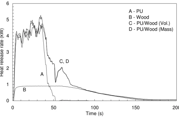
Figure 11. Heat Release Rate for “block” simulations.
Table 5. Parameters for ‘blocks’ simulations.
Simulation Materials Reaction blocks_A Upholstery, Inert PU blocks_B Pine, Inert WOOD blocks_C Pine, Upholstery PU/WOOD (Vol.) blocks_D Pine, Upholstery PU/WOOD (Mass)
One simple method for combining material properties is to average them on a volumetric basis. For the two equal sized blocks in these simulations, the volumetric average is equivalent to the arithmetic average. Table 6 contains volume-averaged properties for a PU/wood composite material. A more rigorous approach is to use a mass weighted average since all of the physical properties are intensive i.e. associated with mass, not volume. For an intensive property Ni, the composite property Ncomp can be calculated as:
Ncomp = i tot i
N
m
m
∑
(7)where mi is the mass of each material and mtot is the total mass of all materials.
For these simulations:
Ncomp = (mPU/(mPU+mW))NPU + (mW/(mPU+mW))NW
= (ρPUVPU/(ρPUVPU+ρWVW))NPU + (ρWVW/(ρPUVPU+ρWVW))NW (8)
Since VPU = VW:
Ncomp = (ρPU/(ρPU+ρW))NPU + (ρW/(ρPU+ρW))NW (9)
For typical values of ρW = 640 kg/m3 and ρPU = 30 kg/m3:
Ncomp = 0.04478 NPU + 0.9552 NW (10)
Table 6 also contains mass-weighted stoichiometry properties for a PU/wood composite.
Table 6. Stoichiometry properties for ‘blocks’ simulations.
(g/mol) (-) (-) (-) (g/g) (kJ/kg) PROPANE 44 5 3 4 0.01 13 100 WOOD1 87 3.7 3.4 3.1 0.01 11 020 POLYURETHANE2 130.3 7.025 6.3 3.55 0.10 13 100 PU/WOOD (Vol.) 108.65 5.3625 4.85 3.325 0.055 12 060 PU/WOOD (Mass) 88.94 3.849 3.530 3.120 0.01403 11 110
1. Ritchie, et al., 5th IAFSS, C3.4H6.2O2.5
2. Babrauskas, NFPA Handbook, C6.3H7.1NO2.1
The heat release rate and smoke production data were compared for all four simulations (Figure 12). Note that the wood sample did not burn to completion in any of the
simulations. The heat release rate for simulation B (wood only) is much less than for simulation A (PU foam) due to its higher heat of vaporization and lower heat of combustion. The heat release rates for the two combined simulations (C, D) are very similar indicating that the choice of property averaging method does not affect this parameter greatly. However, the smoke yields for the two methods are markedly different with the mass averaging method yielding much lower smoke production rates. From a design point of view, the two methods will yield similar heat release rates, and therefore temperature and velocity fields, but will give drastically different smoke concentrations throughout the simulation.
(Figure)
Figure 12. Smoke production for ‘blocks’ simulations.
Another issue to note when averaging material properties is time averaging. The PU smoke production rate data shows a quick burn producing a large amount of smoke early in the fire. In contrast, the wood simulation yields a lower amount of smoke lasting a longer period of time. Combining the material properties averages the two behaviours, yielding an intermediate smoke production rate for an intermediate amount of time. Although the total amount of smoke produced is roughly the same, analyses which depend heavily on the initial rate of smoke production should be considered carefully.
COMBUSTION MODEL
Two main methods exist for modeling of fire sources using CFD techniques: volumetric heat source modeling and chemical modeling. Volumetric heat source modeling specifies a source of heat and combustion products over a volume in the flow domain. Chemical models such as the mixture fraction model implemented in FDS assume an infinitely fast combustion reaction occurring on an infinitesimally thin flame sheet.
A volumetric heat source model is computationally less expensive than a chemical model. It also requires a lower mesh resolution for the combustion volume, further reducing solution times. Chemical models have the advantage of being able to model fire development directly, as opposed to volumetric heat source models, which require a prescriptive trend for the fire development.
Volumetric heat source models are appropriate for simulations where combustion chemistry has a limited impact on the flow field. This includes plume flow at elevations
above the mean flame height and the movement of heat, smoke and toxic gas in a multi-compartment fire. Validation of volumetric heat source models against experimental data has shown that they can yield accurate results for regions of the flow domain remote from the fire itself [3]. Volumetric heat source models do require an appropriate combustion volume to be chosen in order to produce accurate results.
Detailed chemical models are required for simulations in which combustion chemistry directly affects the fire development, such as flame spread or under-ventilated
compartment fires. Fire growth and fire suppression modeling are highly dependent on combustion chemistry and should not be treated with a volumetric heat source model. A wide variety of combustion chemistry models are available whose application depends on the fuel type and combustion conditions.
INTERFACE HEIGHT
Fire protection engineering designs often require estimates of layer interface height throughout the protected space. Zone models are designed to calculate these layer heights directly in addition to average temperatures in the hot and cold layers. In contrast, CFD models calculate temperatures throughout the flow domain. A physically reasonable method is therefore required to calculate the above three values from CFD data. Reference 8 gives an example of such a method applied to experimental data.
Previous versions of FDS allowed temperature data to be collected at discrete points which could then be processed in the same way as experimental data. This approach required significant data processing. FDS Version 4 applies a numerical integration based on conservation of mass and energy to process any vertical temperature profile into a single interface height. FDS also calculates the hot and cold layer average temperatures. All three values are available as time-varying quantities.
CFD software which makes use of the k-ε turbulence model generally performs poorly when it comes to predicting layer heights [9]. The reason for this is attributed to the differences between large eddy simulations and the k-ε turbulence model. LES models are able to directly model a proportion of the flow eddies.
SOOT MODELLING
FDS models soot as a transported quantity similar to the gaseous combustion products. Soot yields from materials are specified as constants. This simple treatment avoids implementation of a more computationally expensive smoke model. However, the following issues related to smoke modeling are not addressed by FDS:
Soot particle agglomeration: In general, soot particle will tend to stick to each other over
time, resulting in less particles but of larger size. Errors in predicting soot particle size and number may impact on occupant visibility estimates and the predicted effectiveness of both photoelectric and ionization smoke detectors. Deposition of soot particles on solid surfaces is a related issue.
Particle size: Soot particle size varies with fuel type and combustion conditions. Particle
size is a key factor in determining smoke obscuration, therefore occupant visibility and detector efficiency are again impacted.
Flow separation: FDS models soot as a continuous phase, not particles with mass. This
treatment will not predict any separation of the soot from the flow as it changes direction. This may be critical for simulations of ducts or detectors. As a partial solution, FDS allows discrete soot particles to be modelled as Lagrangian particles.
Colour: Soot particle colour varies primarily with fuel type: hydrocarbon soot is much
darker than cellulosic soot, for example. FDS does not allow modeling of soot particle colour. When smoke obscuration is defined purely as light absorption by soot particles, their colour does not have an effect. In reality, light scattering for lighter coloured smokes drastically decreases effective visibility because of lower light coherence. The response of smoke detectors based on backscattering technology will also be difficult to compare to FDS results.
Recommendations for addressing these issues in CFD models are beyond the scope of this paper. The potential impact of these factors on data from CFD analyses should be addressed on a case-by-case basis.
BOUNDARY LAYER MODELING
A fluid’s tangential velocity is zero at any solid surface and increases to the freestream velocity through the boundary layer. Accurate modeling of boundary layers is important for most thermofluid simulations. In full-scale fire simulations, boundary layer modeling mainly affects the transfer of heat from hot combustion gases to solid surfaces. This will in turn influence secondary ignition times, pyrolysis rates, heat losses from
compartments and the development of ceiling and wall layers as they are cooled. Boundary layer modeling may also have an affect on entrainment into ceiling jets.
The importance of boundary layers varies with each fire scenario. For compartment fires, the hot layers may move fast enough to make accurate modeling of the boundary layers relatively unimportant. For lower speed flows, such as ceiling jets from plumes rising over a large elevation, boundary layers have a greater impact on the flow. Scenarios involving very low speed flows such as detector activation modeling may be especially susceptible to errors in boundary layer modeling.
FDS models boundary layer development by applying a tangential velocity boundary condition at fluid-solid interfaces. For gases, most boundary layer thicknesses are in the 10-3 m range. Resolution of such a thin layer for construction-scale simulations is
generally difficult due to the high computational costs. To compensate for this lack of mesh resolution, FDS sets the fluid velocity at solid interfaces to a fraction of its value in the next mesh element away from the wall. In effect, this replaces the boundary layer with a linear approximation. Modelers can specify the tangential velocity fraction to represent anything from a no-slip condition, or zero velocity, to a free slip condition representing no wall friction. Mass and heat transfer at the fluid-solid interface are handled mainly through empirical correlations.
As an option, FDS allows a direct numerical simulation (DNS) to be performed where all flow features are calculated directly without resorting to a turbulence or eddy model. Fluid velocities at solid interfaces are set to zero. Among the benefits are better
However, the required mesh resolution is very high, limiting the use of DNS to small-scale simulations for most modelers.
Any FDS simulations in which heat transfer or wall friction are a major factor should be the subject of a grid sensitivity study focused on the boundary layer. Although physically small, the boundary layer has the potential to impact the rest of the flow.
CONCLUSIONS
This paper deals with the use of CFD models in applications related to fire modelling and smoke movement in enclosures and especially in atria, and tunnels. The aim of the paper is to demonstrate through examples the impact on the solution of some parameters used to define and solve the problem in these models. Key parameters examined include: grid resolution, plume entrainment rates, combustion models, smoke modeling, radiative fraction, non-orthogonal geometries, interface height calculation, and boundary layer modeling.
The results of the examples presented lead to the following conclusions:
The accuracy of plume characteristics for a constant mesh element decreases with increasing fire size.
The results from the ‘atrium’ simulations show that high resolution modelling of the combustion volume may not be necessary for accurate prediction of the bulk plume flow at higher elevations. As a rough guideline, mesh resolutions in the order of 10-1 m should be used for plume models.
Non-isometric mesh elements have an impact on the solution and should be applied carefully. Small aspect ratios produce results similar to isometric meshes, however as the aspect ratios increase the impact on the solution becomes significant.
Flows through doors and windows can be accurately predicted with the addition of an exterior computational domain of small length.
In cases where a non-orthogonal grid is necessary it was found that vorticity compensation in FDS does make a difference in the flow dynamics around non-orthogonal geometries. The use of a non-non-orthogonal gravity vector may also be appropriate for simple geometries.
The radiative fraction affects significantly fire development and time to flashover for a compartment. It should be selected carefully to represent the burning fuel.
When the fuel package is a single object consisting of multiple fuels, the package can be modelled as a block with fuel properties that are computed as a mass weighted average of the constituent fuel properties. Note that the preferred approach is direct modeling of fuel package geometry and composition if sufficient computing resources are available.
REFERENCES
[1] Mills, F.A., Case study of a fire engineered approach to a large, unsprinklered, naturally ventilated atrium building, ASHRAE Transactions, Volume 107, Part 1, 2001.
[2] Sinclair, R., CFD simulation in atrium smoke management system design, ASHRAE Transactions, Volume 107, Part 1, 2001
[3] Yau, R., Cheng, V., Yin, R. Treatment of fire source in CFD models in
performance based fire design. International Journal on Engineering Performance-Based Fire Codes, Vol. 5, No. 3, pp. 54-68. 2003.
[4] McGrattan, K., Forney, G., et. al. Fire Dynamics Simulator (Version 3) User’s Guide. National Institute of Standards and Technology. November 2002.
[5] McGrattan, K., Forney, G. Fire Dynamics Simulator (Version 4) User’s Guide. National Institute of Standards and Technology. July 2004.
[6] SFPE handbook of fire protection engineering, 2nd Ed. National Fire Protection Association. 1995
[7] Ma, T. G., Quintiere, J. G. Numerical simulation of axi-symmetric fire plumes: accuracy and limitations. Fire Safety Journal Vol. 38, Iss. 5, pp. 467-492. September 2003.
[8] He, Y.P., Fernando, A., Luo, M.C. Determination of interface height from
measured parameter profile in enclosure fire experiment. Fire Safety Journal, 31, pp. 19–38. 1998.
[9] Hadjisophocleous, G.V., Lougheed, G.D., Cao, S. Numerical study of the
effectiveness of atrium smoke exhaust systems. ASHRAE Transactions, 105, (1), pp. 699-715. 1999.
Figures
Figure 1. Geometry for ‘plume3’ simulations.
0.0 0.5 1.0 1.5 2.0 2.5 3.0 3.5 0 200 400 600 800 1000 Temperature (°C) Elevation (m) A B C Theo.
0.0 0.5 1.0 1.5 2.0 2.5 3.0 3.5 0.00 0.25 0.50 0.75 1.00 1.25 1.50 Mass flow rate (kg/s)
Elevation (m) C (24 kW) D (48 kW) E (12 kW) Theo. (C) Theo. (D) Theo. (E)
Figure 3. Comparison of ‘plume3’ mass flow rate profiles, various fire sizes.
0 5 10 15 20 25 30 0 50 100 150 200 250 300 350 Mass flow rate (kg/s)
Elevation (m) D
E F G Theo.
Figure 5. Comparison of mass flow rate profiles for ‘atrium’ simulations.
0 1 2 3 4 5 6 7 8 9 10 0 20 40 60 80 100 Temperature (°C) Elevation (m) A (1:1) C (1:5) D (1:10)
Figure 7. Geometry for ‘door plume’ simulations. 0.0 0.5 1.0 1.5 2.0 2.5 0 50 100 150 200 250 300 Temperature (°C) Elevation (m) A B C D
Figure 9. Geometry for ‘slope’ simulations. 0 5 10 15 20 25 30 0 5 10 15 20 25 30 35 40 45 50 55 X-position (m)
Mass flow rate (kg/s
)
A B C D
0 1 2 3 4 5 6 0 50 100 150 200 Time (s)
Heat release rate (kW)
A - PU B - Wood C - PU/Wood (Vol.) D - PU/Wood (Mass) A B C, D
Figure 11. Heat release rates for ‘blocks’ simulations.
0.0E+00 5.0E-07 1.0E-06 1.5E-06 2.0E-06 2.5E-06 3.0E-06 0 50 100 150 200 Time (s) Soot mass (kg) D A C B A - PU B - Wood C - PU/Wood (Vol.) D - PU/Wood (Mass)