When does a developing country use new technologies?

HAL Id: halshs-00197539

https://halshs.archives-ouvertes.fr/halshs-00197539

Submitted on 14 Dec 2007

HAL is a multi-disciplinary open access

archive for the deposit and dissemination of sci-entific research documents, whether they are pub-lished or not. The documents may come from teaching and research institutions in France or

L’archive ouverte pluridisciplinaire HAL, est destinée au dépôt et à la diffusion de documents scientifiques de niveau recherche, publiés ou non, émanant des établissements d’enseignement et de recherche français ou étrangers, des laboratoires

When does a developing country use new technologies?

Olivier Bruno, Cuong Le Van, Benoît Masquin

To cite this version:

Olivier Bruno, Cuong Le Van, Benoît Masquin. When does a developing country use new technologies?. 2005. �halshs-00197539�

Maison des Sciences Économiques, 106-112 boulevard de L'Hôpital, 75647 Paris Cedex 13

http://mse.univ-paris1.fr/Publicat.htm

UMR CNRS 8095

When does a developing country use new technologies ?

Olivier BRUNO, GREDEG Cuong LE VAN, CERMSEM Benoît MASQUIN, GREDEG

When Does a Developing Country Use New

Technologies?

∗

Olivier Bruno

_{, Cuong Le Van}

_{, and Benoît Masquin}

July 6, 2005

Abstract

We develop a model of optimal pattern of economic development that is first rooted in physical capital accumulation and then in tech-nical progress. We study an economy where capital accumulation and innovative activity take place within a two sector model. The first sec-tor produces a consumption good using physical capital and non skilled labor. Technological progress in the consumption sector is driven by the research activity that takes place in the second sector. Research activity which produces new technologies requires technological capital and skilled labor. New technologies induce an endogenous increase of the Total Factor Productivity of the consumption sector. Physical and technological capital are not substitutable while skilled and non skilled labor may be substitutable.

We show that under conditions on the adoption process of new tech-nologies, the optimal strategy for a developing country consist in accu-mulating physical capital first; postponing the importation of techno-logical capital to the second stage of development. This result is due to a threshold effect from which new technologies begin to have an impact on the productivity of the consumption sector. However, we show that once a certain level of wealth is reached, it becomes optimal for the economy to import technological capital to produce new technologies.

∗_{The authors would like to thank the participants to the seminar of GREDEG,}

espe-cially Richard Arena, Flora Bellone, Jean-Luc Gaffard and Jacques Ravix, and also the participants to a seminar in European University Institute

†_{GREDEG, UNSA}

‡_{GREDEG, CERMSEM, CNRS, UNSA, University Paris 1}

1

Introduction

It is still rather unclear whether capital accumulation matters relatively more than technological progress in the growth of developing countries. The Krugman — Solow controversy about the Asian Miracle illustrates par-ticularly well this divergence between those who think that capital accumu-lation is an unimportant part of the growth process and those who think that it is a fundamental factor of growth for developing countries.

According to the traditional growth theories, poorer countries grow faster than richer ones during their first stage of development. This result is rooted in the assumption of decreasing returns to scale on capital accu-mulation which induce a catching-up process compatible with conditional convergence (Cass [1965]). However, cross-countries empirical studies show that development patterns differ considerably between countries in the long run (Barro&Sala-i-Martin [1995], Barro [1997]). These differences can be ex-plained within a model of capital accumulation with convex — concave tech-nology. In such a framework, Dechert and Nishimura [1983] prove the exis-tence of threshold effect with poverty traps explaining alternatively "growth collapses" or taking-off. In all those models, the rate of growth is exoge-nous. Alternatively, other models propose several ways for endogeneizing the rate of growth: they state that growth patterns are influenced by ed-ucational resources, innovation processes and technical differences between countries. Therefore, developing countries initially follow divergent paths of growth corresponding to international differences in factor endowments and in patterns of government intervention. However, this point is in contradic-tion with most of the empirical studies stressing the role played by capital accumulation in early stages of growth.1

According to these empirical studies, it seems that the respective weight of capital accumulation and technical progress which contributes to explain the rate of growth of a country depends on its level of development. The higher the level of development the higher the weight of technical progress, and the smaller the relative share of capital accumulation (Kim and Lau [1994])

Even if this idea seems to be spreading in the profession, it seems there is still no model explaining the optimal switch of a country from the first stage to the second stage of development. In this paper, we present a model

1_{Notice that threshold effect is also used by Le Van and Saglam [2004] who show that}

a developing country can retain to invest in technology if the initial knowledge of the country and the quality of knowledge technology are low or if the level of fixed costs of the production technology are high.

which aims at explaining this switch. We show that the optimal pattern of growth of a developing country is initially determined by physical cap-ital accumulation. Later, the technological progress will appear when the country has reached a certain level of development. Capital accumulation and innovative activity take place within a two sector growth model. The first sector produces a consumption good using physical capital and non skilled labor according to a Cobb-Douglas production function. Technolog-ical progress in the consumption sector is driven by the research activity that takes place in the second sector. Research activity which produces new technologies requires technological capital and skilled labor along the line of a Cobb-Douglas production function. When new technologies produced by the research activity are used in the consumption sector they induce an endogenous increase of the Total Factor Productivity. The two kinds of capital are not substitutable while skilled and non skilled labors may be substitutable.

We suppose that technological capital, used by the research activity, is not produced within the economy. The domestic economy must purchase it in the international market at a given price. Consequently, the consumption good can be consumed, invested as physical capital or exported in order to import technological capital. The price of the consumption good is given by the international market and is used as numeraire in our economy. Finally, we assume that physical capital is less costly than technological capital. Our model exhibits first decreasing returns and then increasing returns, and from this point of view it differs from Dechert and Nishimura [1983] seminal model which is convex-concave.

We show that under conditions on the adoption process of new technolo-gies, the optimal strategy for a developing country consist in accumulating physical capital first; postponing the importation of technological capital to the second stage of development. thus, all resources of the economy are devoted to consumption or investment in the physical capital and there is no research activity. The growth process is initially driven by capital accu-mulation using concave technology. This result is due to a threshold effect from which new technologies begin to have an impact on the productivity of the consumption sector. Indeed, it is necessary to have a minimum amount of adoption of new technologies in order for them to be efficient. This may be due to technological complementarity between new technologies or to a network effect (Ciccone and Matsuyama (1999)). Threshold is related to three factors: the amount of available human capital, the price of techno-logical capital and the initial income of the economy. For given values of these factors, we show that there is a time period after which it is optimal

for the economy to import technological capital in order to produce new technologies. From that date onwards, research activity generates an en-dogenous technical change and the economy follows an optimal enen-dogenous growth path with increasing returns to scale technology. Our model exhibits an optimal pattern of economic development that is first rooted in physical capital accumulation and then in technical progress. As a consequence of the existence of the threshold, a country may never take off and may converge towards a traditional steady state. This explains that the international con-vergence or dicon-vergence of income levels tightly depends on the value of the threshold effect.

The initial value of human capital plays an essential role in the process we have just described. The higher this value, the sooner research activity and endogenous growth will take place. This result is in accordance with the empirical study of Benhabib and Spiegel [1994] showing that growth is related to the initial level of human capital and not to the accumulation of human capital.

In the last part of the model (Section 5) we relax the assumption of non substitutability between the two kinds of labor. We allow high-skilled work-ers to work in the production sector. We show that the optimal endogenous growth path may be compatible with an underutilization of high-skilled la-bor in the research activity. However, if the number of high-skilled workers is low relatively to the low-skilled workers then, after a certain time, the technological sector will full employ high-skilled workers.

Our paper is organized as follows. We set the model in Section 2. We first study the one period economy in Section 3. Section 4 deals with the infinitely lived optimal growth model with non substitutable labor force. In Section 5, we allow high skilled workers shift towards consumption sector but low skilled workers cannot join the innovative sector. Section 6 gathers the main results of our paper.

2

The Structure of the Economy

We consider a developping country which produces a consumption good Yd with physical captial Kd and low-skilled labor Ld. The consumption

sector may use a quantity of new technologies Yeto increase its Total Factor

Productivity. We have:

Yd= φ (Ye) KdαdL1−αd d

where αd∈ (0, 1) and φ is a non decreasing function which verifies φ (0) =

The amount of new technologies Ye may be produced through a

Cobb-Douglas function using technological capital Ke and high-skilled labor Le.

We have:

Ye= AeKeαeL1−αe e.

where αe∈ (0, 1) and Ae is the total productivity.

The economy cannot produce technological capital whereas physical cap-ital and consumption good are homogenous. It exports consumption good Yd in order to import technological capital. We use domestic consumption

good as numeraire. Prices are respectively λ > 1 for technological capital and 1 for consumption good and physical capital.

Let S be the value of the initial wealth of the country in terms of con-sumption good. S could take the form of a development aid granted to the developing economy by foreign countries. It can be either used for physical capital accumulation or for the importation of technological capital. The budget constraint of the economy is:

Kd+ λKe = S

3

The Single Period Model

The social planner maximizes the following program max

c,Ke,Kd,Le,Ld

{u(c)} under the constraints:

c = Yd (1) Yd= φ (Ye) KdαdL1−αd d (2) Ye= AeKeαeL1−αe e (3) Kd+ λKe = S (4) Ld≤ L∗d (5) Le≤ L∗eh (6)

By assumption, the function u is strictly increasing. Thus, maximising agents’ utility is equivalent to maximize the quantity of consumption goods. In a single period model there will be no saving or investment (equation

1). In (5) and (6), L∗_d and L∗_e are exogenous supplies of low-skilled and high-skilled workers. These inequalities state there is no possible transfer between high-skilled and low-skilled workers. We suppose the human capital for high-skilled workers is measured by the number h ≥ 1.

Let θ = λKe

S . Then (4) can be re-written

Kd= (1 − θ) S, λKe= θS (7)

Since at the optimum, Le= L∗eh, Ld= L∗d, the social planner’s problem

turns out to be max θ∈[0,1]φ Ã Aeh1−αeL∗ 1−αe e λαe θ αe_Sαe ! (1 − θ)αd_Sαd_L∗1−αd d (8) Let re= _λAαee L∗ 1−αe e h1−αe and ψ (re, S, θ) = φ (reθαeSαe) (1 − θ)αdL∗ 1_−αd d

Solving the previous problem becomes equivalent to solve max

0≤θ≤1ψ (re, S, θ) (9)

Since the function ψ is continuous in θ, there will always be an optimal solution. Let be

G(re, S) = Argmax{ψ(re, S, θ) : θ ∈ [0, 1]}

and F (re, S) = max{ψ (re, S, θ) : θ ∈ [0, 1]}. From the Maximum Theorem,

F is continuous, and the maximum output of the consumption sector will be H(re, S) = F (re, S)Sαd.

In this program the function φ is important because it represents the way the research output impacts the economy. Two alternative situations are possible. On the one hand, new technologies may have an immediate impact on TFP. In that case, there is no adoption effect and it is always efficient to use the technological capital. On the other hand, we can assume technological complementarity between new technologies. In that case, a minimum level of adoption of new technologies is necessary in order for them to impact the economy. In the case of adoption effect, the developing country must be sufficiently abundant in resources or human capital in order to take off by buying technological capital.

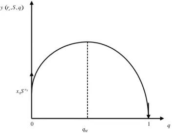
(r Se, , ) y q 0 d x Sa M q q 0 1 Figure 1:

3.1

Case 1: No adoption effect of new technologies

Proposition 1 Assume φ continuously differentiable, strictly increasing and φ0(0) > 0. Then G (re, S) is not empty. Moreover, G (re, S) ⊂ ]0, 1[

Proof. It’s obvious that the function ψ is continuouly differentiable in ]0, 1[ . It satisfies ψ0_θ(re, S, 0) = +∞ and ψ0θ(re, S, 1) = −∞. Hence, there

exist θ1 with ψ(re, S, θ1) > ψ(re, S, 0) and θ2 with ψ(re, S, θ2) > ψ(re, S, 1).

Therefore, the maximizer θM must be included in ]0, 1[.

Figure 1 sketches ψ (re, S, θ) with φ strictly concave. In that case, the

developing economy will devote an equilibrium proportion θM of its initial

wealth to buy technological capital. A share of new technologies is still produced in the economy.

3.2

Case 2: Existence of an adoption effect of new

technolo-gies

In the previous case we suppose that any rise in the quantity of technological capital, even very small, could have a direct effect on TFP of consumption

( )

sector. To analyse the impact of the adoption of new technologies, we assume there is a threshold effect from which new technologies begin to impact positively the TFP. If level of the research activity is not sufficient, it will be useless for the consumption sector.

Assume that the function φ is not strictly increasing but is supposed to have the following form:

φ (x) = ½

x0, ∀x ≤ X

x0+ γ (x) , ∀x ≥ X

¾

with x = reSαeθαe and γ continuously differentiable, γ0 > 0, γ (X) = 0.

Figure 2 sketches φ when γ (x) = ax, a > 0.

The technological capital is useless since reSαe ≤ X.

In the case reSαe > X, there is a ¯θ that satisfies reSαe¯θ = X

We can prove that if S is high enough, it will be efficient to use the technological capital and produce new technologies, and when S is small, it is not efficient to import technological capital.

Proposition 2 _{(i) If S ≤ (r}X

e) 1

αe _{then G (re, S) = {0} .}

Proof. _{(i) If S ≤ (}X_r

e) 1

αe_{, then for any θ ∈ [0, 1], we have reS}αe_θαe

≤ X, and hence ψ(r, S, θ) = x0(1 − θ)αdL∗

1_−αd

d . Obviously, the maximizer is unique

and equals 0.

(ii) Observe that ∀S ≥ 0, F (re, S) ≥ x0L∗ 1_−αd

d . Let S0 > (_rX_e) 1 αe_{, and}

¯

θ(S0) satisfies reS0αeθ(S¯ 0)αe = X. Let ˆθ ∈]¯θ(S0), 1[. When S increases,

¯

θ(S) decreases and ˆθ will be in ]¯θ(S), 1[. We have ψ(re, S, ˆθ) → +∞ when

S → +∞. Hence, for S large enough, say, greater than some ˆS, then maxθ{ψ(re, S, θ)} > x0L∗

1_−αd

d . That implies 0 /∈ G(re, S). Since ψ(re, S, 1) =

0, we have 1 /_{∈ G(r}e, S). The proof is complete.

CommentObserve that the larger re is the higher the opportunity for the

country to use new technology. Therefore, if the number of high-skilled workers is large, or if their human capital is high, or if the price of new technology is low, or if the productivity of the new technology production function is important, then the country will use new technology more rapidly. Finally, we want to prove there exists a critical value Sc_{, i.e., if S < S}c

then G(re, S) = {0} and if S > Sc then G(re, S) ⊂]0, 1[. In that case, the

country will import technological capital and produce new technologies as soon as its wealth S is higher than the critical value Sc_{. Figure 3 illustrates}

that point.

Let B = {S ≥ 0 : F (re, S) = x0L∗ 1_−αd d }.

Lemma 3 B is non empty and compact. Proof. _{(i) B is not empty: obviously, 0 ∈ B.}

(ii) B is closed because the function F is continuous.

(iii) To prove that B is bounded take a sequence Sn converging to +∞.

Fix some θ ∈]0, 1[. For n large enough, ¯θ(Sn) < θ < 1. Then ψ(re, Sn, θ)

converges to +∞. This implies F (re, Sn) > x0 L∗ 1_−αd

d for any n sufficiently

large. That contradicts Sn∈ B.

Proposition 4 Let Sc _{= max{S : S ∈ B}. Then if S < S}c we have G(re, S) = {0} and if S > Sc then G(re, S) ⊂]0, 1[.

Proof. From Proposition 2(i), Sc> 0 since it must be greater than (X_r

e) 1 αe_.

q ( )Sc q c S (e, ) F r S 1 0 d d L-ax S 1 S 2 S 1 2 c S <S <S <S 1 Figure 3:

First, observe that if S < Scthen F (re, S) = x0L∗ 1_−αd

d . Indeed, we have

∀θ ∈ [0, 1], ψ(re, S, θ) ≤ ψ(re, Sc, θ).

Hence F (re, S) = maxθ{ψ(re, S, θ)} ≤ maxθ{ψ(re, Sc, θ)} = F (re, Sc) =

x0L∗ 1_−αd d . Since ∀S ≥ 0, F (re, S) ≥ x0L∗ 1_−αd d , we have F (re, S) = x0L∗ 1_−αd d

Now, (i) if S > Sc, then from the very definition of Sc, we have G(re, S) ⊂

]0, 1[.

(ii) If S < Sc, then take some S0 < Sc. Suppose for S0 we have two solutions

θ1_M = 0 and θ2_M > 0. There must be ¯θ0 ∈]0, 1[ which satisfies reS0αe(¯θ0)αe =

X (if not, ∀θ, reS0αe ≤ X, and G(re, S0) = {0}). For θ ∈]0, ¯θ0], we have

ψ(re, S, θ) = (1 − θ)αdx0L∗ 1_−αd

d < ψ(re, S, 0) = x0L∗ 1_−αd

d . Hence θ2M > ¯θ0.

Let S0 < S1 < Sc, and ¯θ1 satisfy reS1αe¯θ αe 1 = X. Then θ2M > ¯θ0 > ¯θ1. We have φ(reS0αe(θ2M)αe) = x0+ γ(reS0αe(θ2M)αe) φ(reS1αe(θM2 )αe) = x0+ γ(reS1αe(θ2M)αe) > φ(reS0αe(θ2M)αe). We obtain a contradiction x0L∗ 1_−αd d = F (re, S1) ≥ φ(reS1αe(θ 2 M)αe)(1 − θ2M)αdx0L∗ 1_−αd d > φ(reS0αe(θ2M)αe)(1 − θ2M)αdx0L∗ 1_−αd d = F (re, S0) = x0L∗ 1_−αd d .

When the economy is subjected to an adoption effect, the impact of new technologies is not instantaneous on the TFP of consumption sector. Conse-quently, the production and the use of new technologies is highly dependent of the level of wealth of the economy, and it is not always optimal to use them. On the contrary, for a level of wealth lower than Sc_{, it is optimal}

for the developping country to devote all its ressources to physical capital accumulation.

4

The Dynamic Model

4.1

The Model

We consider now an economy with one infinitely lived representative agent who has an intertemporal utility function. She has the possibilty to consume or to save at each period t. Savings are directly used to buy an equivalent amount of capital. This capital as before can be of two kinds, technological

or physical capital. As before, we suppose that the technological capital costs more than the physical capital. There is no change in the production functions of the consumption goods and of the new technology.

4.1.1 The program

The social planner will solve the following program.

max

+∞

X

t=0

βtu (ct) with 0 < β < 1,

under the constraints: for every date t,

ct+ St+1≤ φ (Ye,t) K_d,tαdL(1−α_d,t d), (10)

Ye,t = AeKe,tαeL1−αe,t e, (11)

Ld,t≤ L∗d, Le,t≤ hL∗e, (12)

Kd,t+ λKe,t= St. (13)

The initial resource S0 > 0 is given.

This problem is equivalent to:

max

+∞

X

t=0

βtu (ct)

under the constraints: for every date t,

ct+ St+1≤ H (re, St) with H (re, St) = max θ φ (reθ αe_Sαe t ) (1 − θ)αdL∗ 1_−αd d S αd t , and S0> 0 is given.

Recall that, as in the previous section, re= Aeh

1−αe_L1−αe e λαe .

We maintain the assumptions stated in Section 3 on φ. We add for this section:

(H1) The function u is strictly concave, strictly increasing and satisfies

u(0) = 0 and the Inada Condition u0_{(0) = +∞.}

From the Maximum Theorem, H is continuous. It is obviously strictly increasing with respect to S and H (re, 0) = 0.

(i) If S < Sc, then the set of optimal values θM, G(re, S), equals {0}, and

(ii) if S > Sc, then G(re, S) ⊂]0, 1[.

Since the utility function is strictly increasing, at the optimum the con-straints will be binding.

ct= H (re, St) − St+1

A sequence (St)_t=0...∞ is called feasible from S0 ≥ 0 if we have ∀t, 0 ≤

St+1 ≤ H (re, St). Thus the initial program is equivalent to the following

problem max ∞ X t=0 βtu (H (re, St) − St+1)

under the constraints,

0 ≤ St+1≤ H (re, St) , for all t ≥ 0,

with S0 > 0 given.2.

4.2

Properties of the optimal path

In this subsection, we will give some properties of the optimal path of our economy. In particular, we will show it is monotonic and does not converge to 0. Under some stronger conditions, we will show that any optimal path will grow without boundaries. Along this growth path, after a date T , the economy will use new technology to produce consumption goods.

Lemma 5 Every optimal path is monotonic

Proof. Notice that we have the following Bellman equation. Let V be the value-function of the problem. We have

∀S0≥ 0, V (S0) = max {u (H (re, S0) − S) + βV (S) : 0 ≤ S ≤ H (re, S0)}

Let Γ denote the optimal correspondence. From Amir [1996], this corre-spondence is non decreasing, i.e.,

if S₀0 < S0 then ∀S10 ∈ Γ(re, S00), and ∀S1 ∈ Γ(re, S0), S10 ≤ S1.

Hence, any optimal path must be monotonic.

2

We assume that the utility function u is such that the sum

∞

[

t=0

βtu (H (re, St) − St+1)

Proposition 6 Every optimal trajectory (S_t∗) from S0 > 0 cannot converge

to 0.

Proof. Suppose that S_t∗ _{→ 0. Then for t ≥ T, we have: St}∗ < Sc. Hence, ∀t > T, H(re, St∗) = x0L∗

1_−αd

d St∗αd and HS0 (re, St∗) → ∞, because, St→ 0.

As u0_{(0) = +∞, we have Euler equation for t > T ,}

u0(c∗_t) = βu0¡c_t+1∗ ¢H_S0 ¡re, St+1∗

¢ . There exists T0 ≥ T such that for all t ≥ T0 we have HS0

¡

re, St+1∗

¢ β > 1. That implies u0(c∗_t) > u0¡c∗_t+1¢or equivalently, c∗_t+1> c∗_{t ≥ c}∗_T0 > 0. That is contradictory with S_t∗_{→ 0 (because it would have for consequence c}∗_{t → 0) .}

Let us denote by K_d,t∗ and K_e,t∗ respectively the optimal values of the physical and the technological capital stock and let θ∗_t the associated optimal capital share, i.e. K_d,t∗ _{= (1 − θ}∗_t)S_t∗ and λK_e,t∗ = θ∗_tS_t∗.

Proposition 7 Let Ss be defined by x0L∗ 1_−αd

d αd(Ss)αd−1 = _β1. Suppose

Ss > Sc. Let S0 > 0. Then there exists T such that: ∀t > T, G(re, St∗) ⊂

]0, 1[ or equivalently K∗ e,t > 0.

Proof. When S0 ≥ Sc, since the optimal path (St∗) is nondecreasing, we

have ∀t > 0, G(re, St∗) ⊂]0, 1[ or equivalently Ke,t∗ > 0.

Consider the case S0< Sc. If for any t, Ke,t∗ = 0, then the optimal path (St∗)

will converge to Ss(see e.g. Le Van and Dana, [2005], Chapter 2). Since we assume Ss> Sc, there will be t with S_t∗ > Sc. In this case K_e,t∗ > 0 which is contradictory.

So, let T be the first date with S_T∗ > Sc. Since the optimal path (S_t∗) is nondecreasing, we will have K_e,t∗ > 0 for every t > T .

Ss is the steady-state of our economy in the case of concave technology. If the critical value from which the economy becomes to import technological capital and to produce new technologies (Sc) is higher than the steady-state value, the economy will never take off. In fact it will converge to its steady-state with a constant value of income per capita. On the contrary, if the steady-state value is higher than the critical wealth from which the econ-omy produces new technologies, it will follow an endogenous growth path with a constant increase in income per capita. Sc depends on the quantity of high-skilled labor and human capital initially available in the economy. Consequently, the model is able to explain different patterns of economic development according to the initial value of these variables. Moreover, it

S s S c S (e, ) H r S Figure 4:

is possible for a country to exhibit in the first stage of its development con-ditional convergence to its steady-state and after a certain period of time a complete divergence. Figure 4 gives a graphical interpretation of proposition 7.

We will show in the case of Ss> Scthat the optimal path S_t∗ may converge to +∞ with θ∗t → θ∞ = αeα+αe d. Thus, the optimal capital stocks converge

also to +∞.

We will now assume

(H2) The function φ has the following form

φ (x) = ½

x0, ∀x ≤ X

x0+ a(x − X), ∀x ≥ X with a > 0.

¾

Lemma 8 Assume (H2). (i) The function F (re, S) is continuously

differ-entiable with respect to S in ]0, Sc[S]Sc_{, +∞[. At S}c, it has left derivative (equal to 0) and right derivative.

(ii) For S > Sc, there exists a unique θM(S) ∈ G(re, S). Moreover, when S

Proof. (i) (a) When S < Sc, from Proposition ??, we have F (re, S) =

x0L∗_d1−αd.

(b) Consider the case where S > Sc. Let ¯θ(S) satisfy reSαe¯θ(S) αe = X. Since ψ(re, S, θ) = x0(1 − θ)αdL∗ 1_−αd d ≤ x0L∗ 1_−αd

d when θ ≤ ¯θ(S), from the

very definition of Sc, any solution must be larger than ¯θ(S). Thus, any solution θ must be interior to the interval ]¯θ(S), 1[, because ψ(re, S, 1) = 0.

The solution is unique since ψ(re, S, θ) is strongly concave in θ. One can

check that ∂ψ_∂θ < 0. It satisfies ψ0_θ(re, S, θ) = 0. Tedious computations give:

αe αd θαe−1 (1 − θ) = x_ar0− aX eSαe + θαe ₍₁₄₎

The left side member is a decreasing function in θ while the right side one is increasing in θ. The solution θM is unique. One can check that

dθM dS = A B (15) with A = aX−x0 are S αe−1_{and B =} αe−1 αd θ αe−2 M −(1+ αe αd)θ αe−1 M < 0. Thus F (re, ·) is differentiable for S > Sc.

(c) When S = Sc, there is a solution θ1_M = 0 and another θ2_M which is the unique solution to equation (14). From Clarke ( [1983] , theorem 2.8.2), there is a right derivative equal to ψ0_S(re, Sc, θ2M) and a left derivative which

is trivially zero.

(ii) In (i) (b), we have shown that G(re, S) is a singleton {θM(S)} when S >

Sc_{. Taking the limit when S → +∞, we obtain that θ}M(S) → θ∞= _αeα_+αe d.

Proposition 9 We maintain the same assumptions as in Lemma 8. We add

(H3) αe+ αd> 1.

There exist ¯Ae > 0 (or ¯h) such that if Ae > ¯Ae (or h > ¯h) then Ke,t∗ →

+∞ and θ∗t → θ∞= αeα+αe d.

Proof. It suffices to show that H_S0(re, S) 6= 1_β, ∀S.

Case 1: x0 − aX < 0. In this case dθM_dS(S) < 0 when S ≥ Sc (see (15)).

Therefore, for every S ≥ Sc, θM(S) > θ∞.

Let θM(Sc) be the unique maximizer associated with F (re, Sc) which is

strictly positive. For short, write θcinstead of θM(Sc). Then (θc, Sc) satisfy

(14) and F (re, Sc) = x0L∗ 1_−αd . We obtain: (x0− aX) αeθαce−1(1 − θc)αd+1 (αe+ αd)θαce− αeθαce−1 = x0.

We see that θc is independent of re hence Ae and h. If Ae (or h) is large

enough, then from (14) Sc_{< S}s _{= (βx} 0αd)

1

1_{−αd and H}0

S(re, S) 6= _β1, ∀S ≤ Sc.

Consider the case where S > Sc. From the envelope theorem and relation 14, we have

H_S0(re, S) = areαeθM(S)αe−1(1 − θM(S))αdSαe+αd−1.

We can bound this derivative from below:

H_S0(re, S) > areαe(1 − θc)αdSαe+αd−1 and hence S < ( 1 βareαe(1 − θc)αd ) 1 αe+αd−1_{, if HS}0_{(re, S) =} 1 β. Again from (14) we can write Sc= (ζ(a,x0,X)

are ) 1

αe _{where the function ζ can be}

easily computed. One can also easily check that if Ae(hence re) is sufficiently

large then S will be less than Sc which is a contradiction.

Case 2: x0− aX > 0. As above, θcis independent of re. If Ae(or h) is large

enough, then from (14) Sc< Ss = (βx0αd) 1 1_{−αd and H}0 S(re, S) 6= _β1, ∀S ≤ Sc. When S > Sc_{, (14), we have θ} M(S) < θ∞. We then have H_S0(re, S) > areαe(1 − θ∞)αdSαe+αd−1 and hence S < ( 1 βareαe(1 − θc)αd ) 1 αe+αd−1_{, if H}0 S(re, S) = 1 β. Apply the same argument as above to obtain a contradiction.

Case 3: x0= aX. From (14), we have θM(S) = θ∞, ∀S ≥ Sc. It is easy to

check that Scαe_ar eθ∞ α e_{(1 − θ}∞₎αd_{= x} 0.

Obviously, when Ae or h are large then Sc < Ss. Since we now have for

S > Sc, H(re, S) = areθ∞ α e_{(1 − θ}∞₎αd_L∗(1−αd)_Sαe+αd we get H_S0(re, S) = areθ∞ α e_{(1 − θ}∞₎αd_L∗(1−αd)_(α e+ αd)Sαe+αd−1

5

Mobility of labour

We now assume that high-skilled people can work in the sector of consump-tion good if the demand for high-skilled labor is not sufficient in the research sector. But the reverse is not possible, i.e. low-skilled people cannot move in the new technology sector. We therefore replace the constraints labor demands (5,6) by

Ld≤ L∗e+ L∗d (16)

and

Le≤ hL∗e (17)

We can write Le= µhL∗e, Ld= L∗d+(1−µ)L∗ewith µ ∈ [0, 1]. We assume that

when the high-skilled workers are in the consumption sector their human capital equals the one of this sector.

The production function in the new technology sector will be: Ye=

Ae

λαeθ

αe_Sαe_µ1−αe_h1−αe_L∗1−αe e

where µ represents the part of high skilled labor used in this sector. The production function in the consumption good sector now is:

Yd= φ (Ye) (1 − θ)αdSαd(L∗d+ (1 − µ) L∗e)1−αd

5.1

The one period model

Let re = _λAαee h1−αeL∗ 1−αe

e . The program of the social planner is:

max 0 ≤ θ ≤ 1 0 ≤ µ ≤ 1 Yd= φ ¡ reθαeSαeµ1−αe¢(1 − θ)αdSαd(L∗_d+ (1 − µ) L∗e)1−αd. Let ϕ (re, S, θ, µ) = φ ¡ reθαeSαeµ1−αe ¢ (1 − θ)αd_(L∗ d+ (1 − µ) L∗e)1−αd.

The problem is equivalent to max

(θ,µ)∈[0,1]×[0,1]ϕ (re, S, θ, µ) .

Let

F (re, S) = max

Then F (re, S) ≥ x0(L∗_d+ L∗e)1−αd. As before, define B = {S ≥ 0 : F (re, S) =

x0(L∗_d+ L∗e)1−αd}. It is easy to check that B is compact and nonempty. The

critical value is

Sc_{= max{S : S ∈ B}} Observe that for S > Scthe function

Z(re, S, θ, µ) = Log(ϕ(re, S, θ, µ))

is strongly concave in (θ, µ). Since to maximize ϕ(re, S, θ, µ) is equivalent

to maximize Z(re, S, θ, µ) when S > Sc, the solution (θM(S), µM(S)) will

be unique. Obviously, if S > Sc _{then θ}

M(S) > 0 (if not, we will have

µ_M(S) = 0 and F (re, S) = x0(L∗_d+ L∗e)1−αd). We have the following result

Proposition 10 Assume L∗e L∗

d < 1−αe

1−αd. Then there exists ¯S such that if S >

¯

S then µ_M(S) = 1.

Proof. Assume the statement false. Then there exists a sequence (Sn)

converging to +∞ with µM(Sn) < 1, ∀n. We may assume µM(Sn) → ¯µ ≤ 1

and θM(Sn) → ¯θ. For short, write µn= µM(Sn) , θn = θM(Sn). For every

n, we have

x0+ a(reSnαeθαneµ1−αn e− X)(1 − θn)αd(L∗d+ (1 − µn)L∗e)1−αd

≥ x0+ a(reSnαeθαeµ1−αe− X)(1 − θ)αd(L∗d+ (1 − µ)L∗e)1−αd

for every θ ∈ [0, 1], every µ ∈ [0, 1]. This inequality is equivalent to x0 Sαe n + a(reθαneµ1−αn e− X Sαe n )(1 − θn )αd_(L∗ d+ (1 − µn)L∗e)1−αd ≥ x0 Sαe n + a(reθαeµ1−αe − X Sαe n )(1 − θ) αd_(L∗ d+ (1 − µ)L∗e)1−αd.

Let Sn converge to infinity. We obtain

are¯θαeµ¯1−αe(1 − ¯θ)αd(L∗d+ (1 − ¯µ)L∗e)1−αd

≥ areθαe µ1−αe(1 − θ)αd(L∗d+ (1 − µ)L∗e)1−αd > 0 if θ ∈]0, 1[, µ > 0.

That implies ¯_{θ ∈]0, 1[, ¯µ > 0. But for every n we also have:}

x0+ a(reSnαeθαneµ1−αn e− X)(1 − θn)αd(L∗d+ (1 − µn)L∗e)1−αd

Since µ_{n∈ (0, 1) we get the first order condition for µn}: areθαne(1 − αe)µn−αe(L∗d+ (1 − µ)L∗e) = L∗_{e(1 − α}d)[ x0− aX Sn + areθαneµ1−αn e].

Let Sn converge to infinity. We obtain ¯µ = (1−αe )(L∗ d+L∗e) (2−αe−αd)L∗e . And ¯µ > 1 if L∗ e L∗ d < 1−αe

1−αd. That implies µn= 1 for any n large enough.

Proposition 11 Let S > Sc. Assume L∗e L∗

d < 1−αe

1−αd and x0− aX ≤ 0. Then

µ_M(S) = 1.

Proof. To make short, write (θM, µM) instead of (θM(S), µM(S)). If

(θM, µM) are interior we have the following first-order conditions

θαe−1 M µ1−α e M αe(1 − θM) = ∙ x0− aX areSαe + θαe Mµ1−α e M ¸ αD, (18) θαe Mµ−α e M (1 − αe)(L∗d+ (1 − µM)L∗e) = ∙ x0− aX areSαe + θαe Mµ1−α e M ¸ (1 − αd)L∗e.(19)

If x0− aX ≤ 0, then from (19) we obtain µM ≥ µ∞ = (1−α

e)(L∗_d+L∗e) (2−αd−αe)L∗e . But if L∗e L∗ d < 1−αe 1−αd, then µ

∞_{> 1 and we have a contradiction. Since µ}

M > 0, we

must have µ_M = 1.

5.2

The Dynamic Model

Define

L(re, S) = F (re, S)Sαd.

The function L is strictly increasing in S, continuous and L(re, 0) = 0.

As before the optimal growth model is:

max

+∞

X

t=0

βtu (L (re, St) − St+1)

under the constraints

0 ≤ St+1≤ L (re, St) S0 > 0 is given.

As in the previous dynamic model, from Amir (1996), the optimal path (S∗ t)

is monotonic.

Proposition 12 Let Ss satisfy

αd(Ss)αd−1x0(L∗e+ L∗d)1−αd =

1 β.

Assume Ss > Sc. Then any optimal path (S_t∗) from S0> 0 cannot converge

to zero. Moreover, there will be a date T such that, for all t > T , the optimal technological capital stock satisfies K_e,t∗ > 0.

Proof. If the optimal path (S∗

t) converges to zero, then for all t large

enough, we have S_t∗ < Sc. That implies the optimal values θ∗t and µ∗t are

respectively 0 and 1. To end the proof, see the proofs of Propositions 6, 7. Observe that along an optimal path, we cannot ensure the supply of high-skilled labor supply be exhausted. The following proposition gives a condi-tion for which that will be true.

Proposition 13 Assume that the optimal path (S_t∗_{) converges to +∞ and}

L∗ e L∗

d < 1−αe

1−αd. Then there exists T such that ∀t > T, µ ∗ t = 1.

Proof. That is a corollary of Proposition 10 Finally we have the following proposition.

Proposition 14 (i) Assume (H3). Then there exists ¯Ae > 0 (or ¯h) such

that if a = ¯a, Ae> ¯Ae (or h > ¯h) then Ke,t∗ → +∞ and θ∗t → θ∞= αeα+αe d.

(ii) Moreover, if L∗e L∗

d < 1−αe

1−αd, then there exists T ≥ 0, such that µ ∗

t = 1 for

every t ≥ T .

Proof. (i) The proof is similar to the one of Proposition 9.

(ii) When x0− aX ≤ 0 then from Proposition 11, we have µ∗t = 1 for every

t ≥ 0. When x0− aX > 0, apply Proposition 13.

Remark 15 Consider the case where x0 = aX and αe+ αd > 1. From

the first order conditions (18, 19) when S > Sc, we obtain that the optimal values (θ∗, µ∗_{) are independent of S and respectively equal}

θ∞= αe αe+ αd , µ∞= (1 − αe)(L ∗ d+ L∗e) (2 − αd− αe)L∗e . The technological function of the optimal growth model becomes

and

L(re, S) = areθ∞ αe

(1−θ∞)αd_µ∞1−αe_(L∗

d+(1−µ∞)L∗e)1−αdSαe+αd−1, if S > Sc.

The function L(re, ·) is concave-convex and differs from the case in Dechert

and Nishimura (1983) where the technology is convex-concave.

6

Conclusion

We summarize the results we obtain in this paper.

1. When there is an adoption effect of new technologies by firms, there exists a critical value Sc for the domestic resource. Below this value, it is not optimal for the country to invest in new technology. Above this value, it is optimal to invest in new technology. The critical value decreases when the human capital or/and the productivity of the new technology sector is high, or/and the price of the new technology capital is low.

2. When the human capital is high and/or the productivity of the new technology sector is high, in the dynamic setting, there is a date T1 such

that for any date beyond T1 the country will adopt the new technology and

grows without bound.

3. If we allow the high skilled workers to move to the consumption sector, then may be a date T2 such that the new technology sector will use all the

high skilled workers only after this date. This result shows that is not always optimal to have a very large number of high-skilled workers.

4. Here we want to sketch a country which faces the corruption phenomenon. There are many ways to formalize this phenomenon. One is to assume that the production function in the consumption sector exhibits fixed costs. But it will raise many mathematical complications. So, we use the way proposed by Dimaria and Le Van (2002). We assume that at every date t, the bribers divert a fraction η ∈ (0, 1) of national resource, St+1, devoted to the next

period investment. The amount ηSt+1 either goes abroad or is used for

consuming imported goods. In this case the constraints at every period are: ct+ St+1= L(re, (1 − η)St)

and

Kd,t+ λKe,t= (1 − η)St.

It is obvious that the new critical value S0c _equals Sc

1−η, i.e. larger than S c_{. It}

converges to +∞ when η goes to 1. The new value S0s (corresponding to the steady state of the optimal growth model without new technology) will be

Ss_{(1 − η)}1_−αdαd _{, i.e. smaller than S}s_{. It converges to zero when η converges}

to one. Assume the initial wealth S0 satisfy Sc < S0 < Ss allowing the

country to take off. In presence of high corruption (η close to 1), we have S0s

< S0< S0 c

and the country will fall down by converging to S0s

.

Observe that in this paper we obtain an optimal path which grows without bound in contrast with usual Ramsey models. Our condition is the same as in Kamihigashi and Roy (2005) for a more general setting.

References

[1] Amir, R., Sensitivity Analysis in Multisector Optimal Economic Mod-els, Journal of Mathematical Economics, 25, pp. 123-141, 1996.

[2] Barro, R. Determinants of Economic Growth. A Cross-Country Empir-ical Study. MIT Press, Cambridge, 1997.

[3] Barro, R. and Sala-i-Martin, X., Economic Growth, McGraw Hill, New York, 1995.

[4] Benhabib, J. and Spiegel, M.M., The Role of Human Capital in Eco-nomic Development: Evidence from Aggregate Cross-Country Data, Journal of Monetary Economics, 34,2, 1994.

[5] Cass, D., Optimal Growth in an Aggregative Model of Capital Accu-mulation, Review of Economic Studies, 32, 1965.

[6] Ciccone, A and Matsuyama, K., Efficiency and Equilibrium with Dy-namic Increasing returns due to Demand Complementarities, Econo-metrica, 67,2, 1999.

[7] Clarke ,F.H., Optimization and Nonsmooth Analysis, John Wiley and Sons, 1983.

[8] Dechert, W.D. and Nishimura, K., A Complete Characterization of Op-timal Growth Paths in an Aggregated Model with a Non-Concave Pro-duction Function, Journal of Economic Theory, 31, pp. 332-354,1983. [9] Dimaria, Ch-H. and Le Van, C., Optimal Growth, Debt, Corruption

and R-D, Macroeconomic Dynamics, 6, pp. 597-613, 2002.

[10] Kamihigashi, T., and Roy, S., A Nonsmooth, Nonconvex Model of Op-timal Growth, 2005 (to appear in Journal of Economic Theory).

[11] Kim, J., and Lau, L., The Sources of Economic Growth in the East Asian Newly Industrial Countries, Journal of Japanese and Interna-tional Economics, 8, 1994.

[12] Le Van, C. and Dana, R.A., Dynamic Programming in Economics, Kluwer Academic Publishers, 2003.

[13] Le Van, C. and Cagri Saglam, H., Quality of Knowledge Technology, Re-turns to Production Technology, and Economic Development, Macro-economic Dynamics, 8, 147-161, 2004.