BRIGHT METAL-POOR STARS FROM THE HAMBURG/ESO SURVEY. II. A CHEMODYNAMICAL ANALYSIS

BRIGHT METAL-POOR STARS FROM THE HAMBURG/

ESO SURVEY. II. A CHEMODYNAMICAL ANALYSIS

The MIT Faculty has made this article openly available. Please share

how this access benefits you. Your story matters.

Citation

Beers, Timothy C. et al. “BRIGHT METAL-POOR STARS FROM THE

HAMBURG/ESO SURVEY. II. A CHEMODYNAMICAL ANALYSIS.”

The Astrophysical Journal 835.1 (2017): 81. © 2017 The American

Astronomical Societ

As Published

http://dx.doi.org/10.3847/1538-4357/835/1/81

Publisher

IOP Publishing

Version

Final published version

Citable link

http://hdl.handle.net/1721.1/109482

Terms of Use

Article is made available in accordance with the publisher's

policy and may be subject to US copyright law. Please refer to the

publisher's site for terms of use.

BRIGHT METAL-POOR STARS FROM THE HAMBURG/ESO SURVEY. II.

A CHEMODYNAMICAL ANALYSIS

Timothy C. Beers1, Vinicius M. Placco1, Daniela Carollo1, Silvia Rossi2, Young Sun Lee3, Anna Frebel4, John E. Norris5, Sarah Dietz1, and Thomas Masseron6

1

Department of Physics and JINA Center for the Evolution of the Elements, University of Notre Dame, Notre Dame, IN 46556, USA;

tbeers@nd.edu,vplacco@nd.edu,dcarollo@nd.edu,sdietz@nd.edu

2

Instituto de Astronomia, Geofísica e Ciências Atmosféricas, Departamento de Astronomia, Universidade de São Paulo, Rua do Matão 1226, 05508-900 São Paulo, Brazil;rossi@astro.iag.usp.br

3

Department of Astronomy & Space Science, Chungnam National University, Daejeon 34134, Korea;youngsun@cnu.ac.kr

4

Massachussetts Institute of Technology and Kavli Institute for Astrophysics and Space Research, 77 Massachusetts Avenue, Cambridge, MA, 02139, USA;afrebel@mit.edu

5

Research School of Astronomy and Astrophysics, The Australian National University, Mount Stromlo Observatory, Cotter Road, Weston, ACT 2611, Australia;john.norris@anu.edu.au

6

Institute of Astronomy, University of Cambridge, Madingley Road, CB3 0HA, Cambridge, UK;tpm40@ast.cam.ac.uk

Received 2016 September 28; revised 2016 November 9; accepted 2016 November 11; published 2017 January 19

ABSTRACT

We obtain estimates of stellar atmospheric parameters for a previously published sample of 1777 relatively bright ( < <9 B 14) metal-poor candidates from the Hamburg/ESO Survey. The original Frebel et al. analysis of these

stars was able to derive estimates of[Fe/H] and [C/Fe] only for a subset of the sample, due to limitations in the methodology then available. A new spectroscopic analysis pipeline has been used to obtain estimates of Teff,log g,

[Fe/H], and [C/Fe] for almost the entire data set. This sample is very local—about 90% of the stars are located within 0.5 kpc of the Sun. We consider the chemodynamical properties of these stars in concert with a similarly local sample of stars from a recent analysis of the Bidelman and MacConnell“weak metal” candidates by Beers et al. We use this combined sample to identify possible members of the halo stream of stars suggested by Helmi et al. and Chiba & Beers, as well as stars that may be associated with stripped debris from the putative parent dwarf of the globular cluster Omega Centauri, suggested to exist by previous authors. We identify a clear increase in the cumulative frequency of carbon-enhanced metal-poor (CEMP) stars with declining metallicity, as well as an increase in the fraction of CEMP stars with distance from the Galactic plane, consistent with previous results. We also identify a relatively large number of CEMP stars with kinematics consistent with the metal-weak thick-disk population, with possible implications for its origin.

Key words: Galaxy: kinematics and dynamics – Galaxy: stellar content – stars: abundances – stars: carbon – stars: Population II– stars: kinematics and dynamics

Supporting material: machine-readable tables

1. INTRODUCTION

There have been numerous recent studies of the disk system of the Milky Way, primarily based on data from the Sloan Digital Sky Survey(SDSS; York et al.2000), in particular the

SEGUE (Yanny et al. 2009) and APOGEE (Majewski

et al. 2015) sub-surveys, as well as from the Radial Velocity

Experiment (RAVE; Steinmetz et al. 2006; Kordopatis et al. 2013) and the Gaia-ESO survey (Gilmore et al. 2012; Guiglion et al. 2015). Beers et al. (2014) and Guiglion et al.

(2015) summarize the pertinent papers, to which the interested

reader is referred. Most of these papers model the Galactic disk system in terms of a superposition of a thin disk, a thick disk, and (in some cases) a metal-weak thick disk (MWTD). The series of papers from Bovy and collaborators, culminating with Bovy et al. (2015), has taken a different approach. These

authors use abundance information ([Fe/H] and [α/Fe]) for large samples of red-clump stars measured with APOGEE to model the radial and vertical structure of the disk in terms of mono-abundance populations (MAPs), and demonstrate that this technique captures the relevant observations without invoking a separation of stellar populations. Because MAPs are based on red-clump stars, they do not include any stars with

< -Fe H 1.0

[ ] and so are not suitable for exploring issues relating to the MWTD, which Beers et al.(2014) have argued

to be a potentially separate component of the disk system that has yet to be explored in detail. A recent paper by Kawata & Chiappini (2016) emphasizes that the separability of the thin

disk and thick disk remains uncertain, arguing that the scheme of chemically dividing the disk system on the basis of the [α/Fe] ratio, pioneered by Lee et al. (2011a,2011b), is for now

the most practical approach.

One of thefirst large spectroscopic samples of stars in the disk system was originally reported by Frebel et al. (2006; hereafter, PaperI). These stars, selected from partially saturated

objective-prism spectra from the Hamburg/ESO survey (HES; Wisotzki et al.2000; Christlieb2003) with 9 < <B 14, formed the basis of an early effort to identify bright metal-poor halo stars in the Galaxy. Due toflaws in the selection procedure, the great majority of these stars turned out to have metallicities more typical of the disk system than of the halo. Even so, the star HE1327-2326, which was first identified in that effort, turned out to have one of the lowest iron abundance known ([Fe/H] = −5.45; Frebel et al. 2005; Aoki et al.2006), only

recently surpassed by SMSSJ031300.36−670839.31, with <

-Fe H 7.8

[ ] (Keller et al.2014; Bessell et al. 2015). That

paper was also thefirst to suggest an increase in the fraction of carbon-enhanced metal-poor(CEMP) stars (Beers & Christlieb

2005) with distance from the Galactic plane, which was later © 2017. The American Astronomical Society. All rights reserved.

confirmed with much larger samples of stars from SDSS (Carollo et al.2012).

A substantial fraction of very low metallicity stars in the halo of the Milky Way have been found to be CEMP stars. Beers & Christlieb(2005) originally divided such stars into several

sub-classes, depending on the nature of their neutron-capture element abundance ratios—CEMP-s, CEMP-r, CEMP-r/s, and CEMP-no.7 As discussed by those authors and many others since, the observed differences in the chemical signatures of the sub-classes of CEMP stars are thought to arise from differences in the astrophysical sites responsible for the nucleosynthesis products they now incorporate in their atmospheres, including elements produced by the veryfirst generations of stars.

At the time PaperIwas published, the authors could obtain

estimates of [Fe/H] and [C/Fe] from their spectra only for those stars with[Fe H]< -1.0, due to the nascent saturation of the CaIIK line. This limitation precluded a comprehensive investigation of the disk system, including stars over the full range of expected metallicities. Over the course of the past decade, we have developed and tested new spectroscopic tools (primarily for application to SDSS stellar spectra—the SEGUE Stellar Parameter Pipeline, SSPP) that are useful for the analysis of stars over wide ranges of [Fe/H] (see, e.g., Lee et al. 2008a). In this paper, we employ a modification of

the SSPP that can be used for spectra of similar resolving power and with input broadbandV B, -V and/or J J, -K

photometry, to obtain estimates of the stellar atmospheric parameters Teff, log g, and [Fe/H], as well as [C/Fe]

abundance ratios for most of the stars in the Paper Isample.

Similarly determined quantities from the local sample of “metal-weak” candidates from Bidelman & MacConnell (1973), reported recently by Beers et al. (2014), are analyzed

in concert with the PaperIsample.

This information (in combination with well-determined radial velocities and available accurate proper motions) is employed to carry out a detailed examination of the kinematics of the combined sample and identify stars that are possible members of the halo stream/trail of stars by Helmi et al. (1999)

and Chiba & Beers (2000), as well as stars that may be

associated with stripped debris from the putative parent dwarf of the globular cluster Omega Centauri (ω Cen), suggested to exist by Dinescu(2002), Klement et al. (2009), and Majewski

et al. (2012). We identify a clear increase in the cumulative

frequency of CEMP stars as a function of declining metallicity, as well as an increase in the fraction of CEMP stars with distance from the Galactic plane, as quantified by the maximum distances reached during the course of their orbits, Zmax,both consistent with previous results. We also identify a number of CEMP stars that are apparently associated with the MWTD, with implications for its origin. Finally, we make use of the Yoon–Beers diagram of A(C) versus [Fe/H] (Figure 1 of Yoon et al. 2016) to sub-classify the relatively small number of

CEMP stars in the combined sample with available kinematic information(36 stars) into likely CEMP-s and CEMP-no stars, and show that the distributions of their Zmaxdiffer, in the sense

that the CEMP-s stars appear to be preferentially associated with the inner-halo population, while the CEMP-no stars are more likely to be associated with the outer-halo population, similar to the previous claim of Carollo et al.(2014).

2. SAMPLE STARS AND ADOPTED PHOTOMETRY Paper Idescribes the original motivations and selection of

the bright candidate metal-poor stars from the HES, to which the interested reader is referred for details. Unfortunately, the original candidate selection was confounded by (known) saturation effects on the derived estimates of approximate B−V to such a degree that numerous stars were included that later turned out to be more metal-rich than hoped for. In spite of this limitation, more than a hundred relatively bright very metal-poor (VMP; [Fe H]< -2.0) stars were identified during follow-up spectroscopy, which formed the basis for much of the analysis carried out in PaperI.

In the present paper, we re-analyze medium-resolution (R∼2000) spectroscopy of the sample of stars from PaperI

(see Table 6 of Paper Ifor the telescope/spectrographs

employed), using the n-SSPP spectroscopic pipeline described below. This new effort, which also incorporates a large amount of newly available broadband V B, -V

photometry for the sample stars, enables determinations of stellar atmospheric parameters for the great majority of the Paper Isample, including stars with metallicities up to solar

and beyond(which were not previously possible), as well as refined estimations of [C/Fe] abundance ratios for most of the stars in this sample.

2.1. Broadband Photometry and Reddening Estimation Broadband V magnitudes and B−V colors for the majority of our program objects were obtained from the APASS database (Henden et al. 2015), supplemented by

photometry from a number of sources as described in Paper I(primarily stars that were re-discoveries of

metal-poor candidates from the HK survey; Beers et al. 1985,

1992). For stars that are of particular interest, i.e., those found

in Paper Ito have [Fe H]< -2.0 or to exhibit enhanced carbon, we also make use of photometry reported by Beers et al. (2007). In a number of cases, we have also used

photometry from the SIMBAD database. For stars with photometry available from multiple sources, we either use the data judged to be superior, or else average data expected to be of similar precision. Near-IR JHK photometry from the 2MASS catalog(Skrutskie et al.2006) is available for all but

a few stars in our sample.

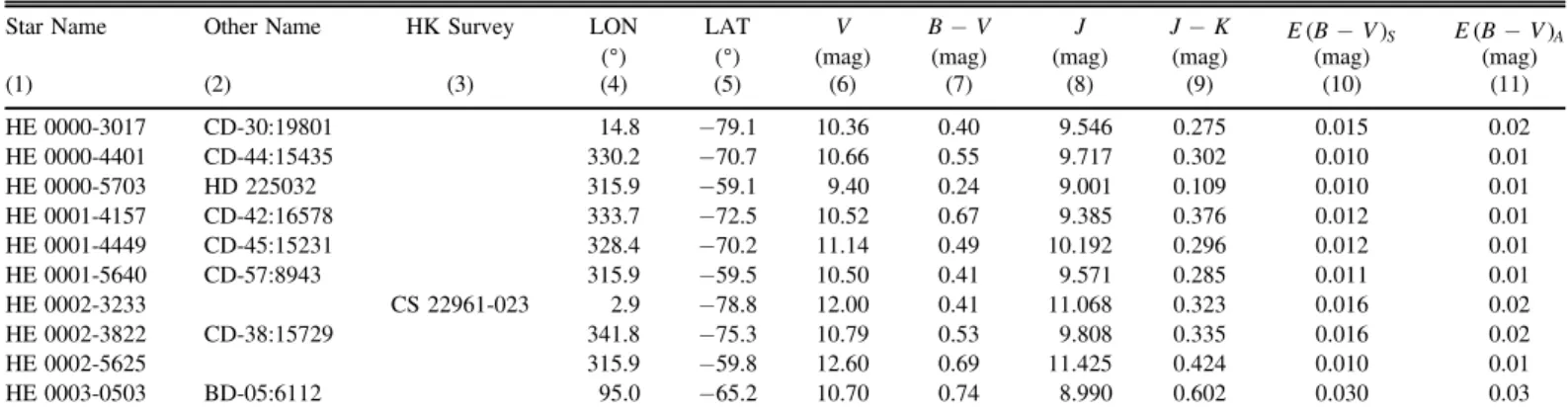
Column(1) of Table1lists the star names, while columns(2) and (3) list other common names for the star and the HK Survey star name, respectively. The full set of coordinates for our program stars are provided in PaperI.Columns (4) and (5) list the Galactic longitude and latitude for our program stars. The adopted V magnitude and B−V colors are provided in columns (6) and (7). The 2MASS J magnitude and J−K colors (including only stars without flags indicating potential problems in the listed values) are listed in columns (8) and (9). In order to obtain absorption- and reddening-corrected estimates of the magnitudes and colors, respectively, we initially adopted the Schlegel et al. (1998) estimates of

reddening listed in column(10) of Table1. We have applied corrections to these estimates for stars with reddening greater thanE B( -V)S = 0.10, as described by Beers et al. (2000). The corrected reddening estimates, E B( -V) , are listed inA column(11).

7

CEMP-s:[C/Fe]>+1.0, [Ba/Fe]>+1.0, and [Ba/Eu]>+0.5; CEMP-r: [C/Fe]>+1.0 and [Eu/Fe]>+1.0;CEMP-r/s: [C/Fe]>+1.0 and 0.0<[Ba/Eu]<+0.5; CEMP-no: [C/Fe]>+1.0 and [Ba/Fe]<0.0.

2

3. RADIAL VELOCITIES, LINE INDICES, ATMOSPHERIC PARAMETERS, ABUNDANCE RATIOS, DISTANCES,

AND PROPER MOTIONS

3.1. Measurement of Radial Velocities and Line Indices Radial velocities were (re-)measured for our program stars using the line-by-line and cross-correlation techniques described in detail by Beers et al. (1999) and references

therein. In the process of carrying out this exercise, we found that many of the new measurements differ (in some cases by large amounts) from those originally reported in PaperI,which apparently suffered from transcription difficulties during file exchanges between the authors. The current measurements supersede those values. The spectral resolution of our data is similar to that obtained for the majority of the HK Survey follow-up; thus we expect that the measured radial velocities should be precise to the same level(or better, given the higher signal-to-noise of our present spectra), on the order of 7–10 km s−1 (one sigma). Column (1) of Table 2 is the star name, while column (2) lists notes on the nature of a small number of stars that deviate from the majority(e.g., hot stars, sdB and WD stars, known variable stars, stars with emission lines, extremely late-type stars), which precludes their use in later analysis. We conservatively estimate that our medium-resolution velocities, RVM, listed in column(3) of Table2, are precise to 10kms−1(as validated below).

Roughly one-third of our program objects (614 stars) have had radial velocities determined from the RAVE survey, based on moderate-resolution (R∼7500) spectroscopy in the region of the Ca triplet from Data Release 4(Kordopatis et al.2013).

The RAVE velocities should be more precise than those we obtained from our lower-resolution spectra (Kordopatis et al. 2013 demonstrate that the majority of the RAVE radial velocities are precise to better than 2 km s−1, with a tail going out to∼5 km s−1, and have small zero-point offsets relative to external catalogs). For our purpose we conservatively assume a precision of 5 km s−1 for the RAVE velocities (validated below). We adopt the RAVE velocities for our subsequent analysis, except in cases where flags were raised in the DR4 database indicating potential problems (including possible binary membership). The available RAVE velocities are listed as RVR in column(4) of Table 2. In order to weed out stars with inaccurate RAVE velocities, we have indicated stars with flags suggesting potential problems with parentheses around them. We still adopt these radial velocities for our analysis if

they are within 20 km s−1of the listed RVMvalue. If the RAVE velocities differ by more than this amount and hadflags raised, we assume that the RVM estimates are superior. We indicate such cases by brackets around the listed RVRvalues. In some instances, there are no flags raised, but the RAVE radial velocities differ from our medium-resolution results by more than 20 km s−1; in such cases, we assume the RAVE estimates are superior, and adopt them.

There are 148 stars in our sample (mostly VMP stars and stars of interest for other reasons, such as carbon enhancement) for which radial velocities based on high-resolution spectrosc-opy are available, either in the published literature or based on more recent unpublished observations we are aware of. These are listed as RVH in column (5) of Table2. We adopt these measurements (when available), with assumed errors of 2 km s−1, even in the few cases where they disagree by more than 20 km s−1with either RVMor RVR. Unrecognized binarity may be responsible for a number of these discrepancies.

Figure 1 (left column) compares the medium-resolution

velocities, RVM, with the high-resolution radial velocities, RVH, while the middle column of panels compares RVMwith the moderate-resolution RAVE velocities, RVR(excluding the rejected cases). The right column of panels compares the RAVE velocities with the high-resolution velocities. As can be appreciated from inspection of this figure, there is generally very good agreement between the different sources of radial velocity. The middle row of panels shows the residuals in radial velocity for each comparison, with dark gray and light gray regions indicating the 1σ and 2σ ranges, respectively. Maximum-likelihoodfits to the residuals in radial velocity for each comparison are shown in the lower panels of each column. The RVMversus RVHresiduals exhibit a scatter of 10.7 km s−1 and a small zero-point offset; the RVM versus RVR residuals exhibit a scatter of 8.8 km s−1and a similarly small offset. The RVRversus RVHresiduals exhibit a scatter of 4.7 km s−1and a small offset. Assuming our adopted estimate of the 2 km s−1 precision for the high-resolution radial velocities, our results indicate that the RAVE radial velocities are precise to 4.2 km s−1 (note that this comparison emphasizes metal-poor stars, for which the RAVE velocities are expected to be somewhat less precise than for more metal-rich stars). Adopting this value for the scatter in the RAVE velocities, we estimate that the medium-resolution velocities have a precision of 7.7 km s−1. Compared to the high-resolution velocities, the medium-resolution velocities are estimated to

Table 1

Photometric Information and Adopted Reddening

Star Name Other Name HK Survey LON LAT V B−V J J−K E B( -V)S E B( -V)A (◦_{) (}◦_{) (mag) (mag) (mag) (mag) (mag) (mag)}

(1) (2) (3) (4) (5) (6) (7) (8) (9) (10) (11) HE0000-3017 CD-30:19801 14.8 −79.1 10.36 0.40 9.546 0.275 0.015 0.02 HE0000-4401 CD-44:15435 330.2 −70.7 10.66 0.55 9.717 0.302 0.010 0.01 HE0000-5703 HD225032 315.9 −59.1 9.40 0.24 9.001 0.109 0.010 0.01 HE0001-4157 CD-42:16578 333.7 −72.5 10.52 0.67 9.385 0.376 0.012 0.01 HE0001-4449 CD-45:15231 328.4 −70.2 11.14 0.49 10.192 0.296 0.012 0.01 HE0001-5640 CD-57:8943 315.9 −59.5 10.50 0.41 9.571 0.285 0.011 0.01 HE0002-3233 CS22961-023 2.9 −78.8 12.00 0.41 11.068 0.323 0.016 0.02 HE0002-3822 CD-38:15729 341.8 −75.3 10.79 0.53 9.808 0.335 0.016 0.02 HE0002-5625 315.9 −59.8 12.60 0.69 11.425 0.424 0.010 0.01 HE0003-0503 BD-05:6112 95.0 −65.2 10.70 0.74 8.990 0.602 0.030 0.03

Table 2

Radial Velocities, Line Indices, Atmospheric Parameters, and Type Assignments

Star Name Note RVM RVR RVH KP HP2 GP TeffS log gS [Fe/H]S TeffR log gR [Fe/H]R TeffH log gH [Fe/H]H TeffC log gC [Fe/H]C TYPE

(kms−1_{) (kms}−1_{) (kms}−1_{) (Å) (Å) (Å) (K) (cgs) (K) (cgs) (K) (cgs) (K) (cgs)} (1) (2) (3) (4) (5) (6) (7) (8) (9) (10) (11) (12) (13) (14) (15) (16) (17) (18) (19) (20) (21) HE0000-3017 21.8 ... ... 6.57 4.99 1.89 6666 3.99 −0.18 ... ... ... 6875 4.60 +0.23 6776 4.41 +0.20 D HE0000-4401 −1.0 −2.1 ... 8.29 3.60 3.55 6199 3.77 −0.13 6168 4.12 −0.05 ... ... ... 6227 4.14 +0.26 D HE0000-5703 30.3 26.4 ... 2.59 9.37 1.16 7758 4.08 −0.03 7474 4.25 −0.10 ... ... ... 8060 4.53 +0.30 D HE0001-4157 2.0 −10.8 ... 9.15 1.73 5.47 5725 3.81 −0.10 5710 3.99 +0.10 ... ... ... 5670 4.19 +0.30 D HE0001-4449 5.0 −9.4 ... 7.53 3.53 2.92 6227 3.65 −0.58 5959 3.66 −0.62 ... ... ... 6260 3.99 −0.28 TO HE0001-5640 −14.0 [23.3] ... 7.80 4.06 2.82 6377 3.86 −0.26 6176 3.65 +0.14 ... ... ... 6436 4.25 +0.11 D HE0002-3233 61.1 ... ... 1.30 4.24 0.48 6349 3.65 −2.54 ... ... ... ... ... ... 6404 4.00 −2.70 TO HE0002-3822 −8.0 ... ... 7.80 3.39 3.20 6132 3.87 −0.59 ... ... ... ... ... ... 6148 4.26 −0.30 D HE0002-5625 22.4 ... ... 9.25 1.65 5.55 5750 4.02 −0.14 ... ... ... ... ... ... 5699 4.45 +0.25 D HE0003-0503 30.6 34.4 ... 6.82 3.39 4.21 5972 2.63 −1.10 (4793) (3.46) (−0.19) ... ... ... 5960 2.72 −0.92 G Note. Parentheses around a listed quantity indicate that it is regarded with some suspicion, while brackets indicate that it is considered as possibly flawed. See text for more details.

(This table is available in its entirety in machine-readable form.)

4 The Astrophysical Journal, 835:81 (22pp ), 2017 January 20 Beers et al.

have a precision of 10.5 km s−1. These values justify our adopted estimates for the kinematic analysis carried out below —sRVR = 5 km s

−1 _{and s = 10}

RVM km s

−1 _{for the RAVE and} medium-resolution velocities, respectively.

For each star, the measured(geocentric) radial velocities are used to place a set of fixed bands for the derivation of line-strength indices, which are the pseudo-equivalent widths of prominent spectral features. We employ a subset of the bands listed in Table 1 of Beers et al. (1999).8Although we do not make use of them in the present analysis, others may choose to, so we list line indices for prominent spectral features in each of our program stars in columns(6)–(8) of Table2. A number of our stars have had more than one spectrum obtained during the course of our follow-up observations. From a comparison of the stars with repeated measurements, we estimate that errors in the line indices on the order of 0.1 Å are achieved. Note that our line indices are identical to those reported in Paper I.

3.2. Stellar Atmospheric Parameter Estimates and Abundance Ratios

In a series of papers, Lee et al. (2008a, 2008b, 2011a),

Allende Prieto et al. (2008), and Smolinski et al. (2011)

describe the development, testing, and validation of the SSPP software, which has been used to determine atmospheric parameter estimates for over 500,000 stars from the SDSS and its extensions. Although the spectra of our program stars do not reach as far red as SDSS spectra(and hence we cannot use as many of the independent methods as the SSPP enables), they are of similar resolving power. We have thus modified the SSPP to accept input from our program spectra, which span a range of 3600–4400 Å, 3600–4800 Å, or 3600–5250 Å, depending on the telescope/spectrograph that was used to acquire them. We have also implemented the use of input

-V B, V (and/or 2MASSJ J, -K) photometric information

rather than requiring SDSS ugriz inputs. This new approach, known as the n-SSPP (for non-SEGUE Stellar Parameter Pipeline), makes use of a subset of previously calibrated methods from the SSPP (those that apply to the available wavelength range of the input spectra) to obtain estimates of the fundamental stellar parameters Teff,log g, and[Fe/H]. For

spectra that extend sufficiently redward to include the CH G-band at ∼4300 Å and/or the MgI feature at ∼5175 Å, the n-SSPP can obtain estimates of[C/Fe] and [α/Fe]9as well(if the spectra are of sufficiently high signal-to-noise, S/N). The n-SSPP has already been applied by Beers et al. (2014) to Figure 1. Radial velocity comparison for the program (RVM), RAVE (RVR), and high-resolution (RVH) stars. Upper panels: comparison between the radial velocities. The solid line is the one-to-one line, and the shaded areas represent the 1σ and 2σ intervals around this line (where σ represents the scatter in the residuals shown in the lower panels). Middle panels: residuals between each pair of measurements. The horizontal solid line is the average of the residuals, while the darker and lighter shaded areas represent the 1σ and 2σ regions, respectively. Lower panels: histogram of the residuals in the radial velocity determinations. The values of the mean offset and scatter are the parameters from the Gaussianfit shown.

8

A complete discussion of the choice of bands, the“band-switching” scheme, and the Balmer line index, HP2, which measures the strength of the Hδ lines, is provided in this reference as well.

9 _{This notation is usually defined as an average of [Mg/Fe], [Si/Fe], [Ca/Fe],} and[Ti/Fe].

medium-resolution spectra of stars from the sample of Bidel-man & MacConnell(1973) stars studied by Norris et al. (1985).

The interested reader should consult that paper for additional information on the operation of the n-SSPP.

We apply the n-SSPP to the sample of 1777 stars from Paper I.Unfortunately, the S/Ns for the spectra of our program stars that extend to wavelength regions that include the MgI feature are not generally high enough to enable confident estimation of this abundance ratio (Lee et al.2011a

recommend S/N > 20 or 25, the latter applying to stars with <

-Fe H 1.4

[ ] ); hence we do not report [α/Fe] for our program stars.

The n-SSPP estimates of stellar atmospheric parameters are listed in columns (9)–(11) of Table 2 as TeffS, log gS, and [Fe/H]S. Although according to the tests described by Lee et al. (Lee et al. 2008a,2008b) and Allende Prieto et al. (2008) the

external accuracy of SSPP parameter estimates is expected to be on the order of 150K, 0.30 dex, and 0.25 dex for Teff,log g,

and[Fe/H], respectively, these are based on the availability of SDSS ugriz and the full spectral coverage associated with SDSS spectroscopy, neither of which applies to the present data. We provide an independent test of our expected parameter errors below.

Lee et al. (2013) describes the procedures adopted to

estimate [C/Fe] for SDSS/SEGUE spectra, based on spectral matching against a dense grid of synthetic spectra; these techniques, with different input photometric information, also apply to the n-SSPP. We have recently expanded the carbon grid to reach as low as[C Fe]= -1.5, rather than the limit of

= -C Fe 0.5

[ ] employed by Lee et al.(2013). According to

Lee et al., the precision of [C/Fe] estimates is better than 0.35dex for the parameter space and S/Ns explored by SDSS/ SEGUE spectra. We expect improved results for the application of the n-SSPP to our program spectra, based on their generally higher signal-to-noise(which typically exceeds S/N ∼50 in the region of the CH G-band). We note that Beers et al. (2014)

concluded that the n-SSPP determination of[C/Fe] for spectra with S/N similar to that of our current program achieved a precision(based on empirical comparisons with high-resolution spectroscopic analyses) of ∼0.20dex.

Table3lists the medium-resolution estimates of the[C/Fe] abundance ratios (“carbonicity”) for our program stars in column (3), indicated as [C/Fe]S. For convenience, we have also listed the n-SSPP estimate of [Fe/H]S in column (2).

Column (4) indicates whether the listed measurement is considered a detection, DETECT = “D”; a lower limit, “L”; an upper limit,“U”; or a non-detection, “X,” which indicates either that the star is too hot(or cool) for carbon to be measured from the CH G-band or that the star does not have a reference metallicity determination. Column(5) provides the correlation coefficient, CC, obtained between the observed spectrum and the best-matching[C/Fe] from the model grids, and column (6) lists the equivalent width of the CH G-band, EQW. For an acceptable measurement of this ratio, we require DETECT= “D,” CC  0.7, and EQW  1.2. The latter restriction ensures that stars with very weak carbon features are not spuriously assigned values by the grid search procedure. See Lee et al. (2013) for a further discussion of these quantities. Stars for

which either the CC or the EQW does not meet the minimum value are indicated by a colon attached to the DETECT parameter in column(4). There are 1491 stars listed in Table3

for which acceptable measurements of [C/Fe] are obtained— 1422 are listed as detections, 58 as upper limits, and 11 as lower limits.

3.3. Comparison to Moderate- and High-resolution Spectroscopic Analyses

There are external measurements of stellar atmospheric parameter estimates for 707 stars in our sample from the RAVE DR4 catalog(Kordopatis et al.2013) and another 104 stars for

which atmospheric parameter estimates based on high-resolu-tion analyses are available from a variety of sources, including the SAGA database (Suda et al. 2008, 2011; Yamada et al.

2013) and Frebel (2010), as well as the references listed in the

PASTEL catalog (Soubiran et al. 2010),10 supplemented by determinations that have appeared in more recent studies, or unpublished results from co-authors of this paper. We either adopted the parameter estimates we judged to be superior or, in some cases, took a straight average of the available estimates. The external parameter estimates from RAVE are listed in columns (12)–(14) of Table 2 as TeffR, log gR, and[Fe/H]R. The high-resolution estimates are listed in columns (15)–(17) of that table as TeffH, log gH, and[Fe/H]H.

Table 3

Carbon Abundance Ratios and Absolute Carbon Abundance Estimates

Star Name [Fe/H]S [C/Fe]S DETECT CC EQW [Fe/H]C [C/Fe]C A(C) CEMP

(1) (2) (3) (4) (5) (6) (7) (8) (9) (10) HE0000-3017 −0.18 +0.15 D 0.995 2.33 +0.20 −0.12 8.52 N HE0000-4401 −0.13 +0.08 D 0.996 4.14 +0.26 −0.19 8.50 N HE0000-5703 −0.03 ... X ... ... +0.30 ... ... X HE0001-4157 −0.10 +0.04 D 0.999 6.42 +0.30 −0.23 8.50 N HE0001-4449 −0.58 +0.25 D 0.994 3.26 −0.28 0.00 8.15 N HE0001-5640 −0.26 +0.19 D 0.997 3.48 +0.11 −0.07 8.46 N HE0002-3233 −2.54 +1.29 D: 0.866 0.76 −2.70 +1.11 6.84 U HE0002-3822 −0.59 +0.17 D 0.994 3.66 −0.30 −0.09 8.04 N HE0002-5625 −0.14 −0.03 D 0.999 6.71 +0.25 −0.30 8.38 N HE0003-0503 −1.10 +1.42 D 0.971 5.20 −0.92 +1.25 8.75 C

Note. A colon following the DETECT code indicates that either the CC or the EQW parameter does not meet the minimum required value for confident detection. See text for more details.

(This table is available in its entirety in machine-readable form.)

10

We are aware that an updated version of this catalog, Soubiran et al.(2016),

is now available, but it was published after we completed the bulk of our analysis, and is hence not used for this exercise.

6

Before carrying out comparisons with our own estimates, based on medium-resolution spectra, wefirst check for external parameter estimates that grossly differ from the estimates determined by the n-SSPP. For the external estimates to be considered commensurate with the n-SSPP estimates, reason-able agreement with the effective temperature, Teff, is required,

at a minimum. To implement this pre-filter, we require that the estimated effective temperatures from the external comparisons are within 500K of the n-SSPP estimates and (in the case of RAVE) that there be no other indication of potential problems, such as flags raised in the RAVE DR4 catalog listing. This results in a total of 80 stars with RAVE estimates marked as suspect, indicated in Table 2 with brackets around the individual parameter estimates. Only 9 stars with available high-resolution spectroscopic parameter estimates are suspect by this criterion, and these are marked with parentheses around the individual parameter estimates in the table.

Beers et al.(2014) presented a similar analysis for the sample

of 302 metal-poor candidates from Bidelman & MacConnell (1973) studied by Norris et al. (1985), roughly one-third of

which had external estimates of stellar atmospheric parameters based on high-resolution spectroscopic analyses. Beers et al. used the sample of stars in common to derive empirical corrections to the n-SSPP parameter estimates, which they applied in order to place these estimates on a scale commensurate with that of the high-resolution work. For the convenience of the reader, these corrections are listed below:

= - -

-Fe HC Fe HS 0.232 Fe HS 0.428 , 1

[ ] [ ] ( · [ ] ) ( )

= - - +

TeffC TeffS ( 0.1758 ·TeffS 1062 ,) ( )2

= - - +

g g g

log C log S ( 0.237 log· S 0.523 .) ( )3 The corrected n-SSPP estimates (TeffC, log gC, and [Fe/H]C) for our program stars are listed in columns (18)–(20) of Table 2. Column (21) of this table lists our adopted type classifications, obtained as described below.

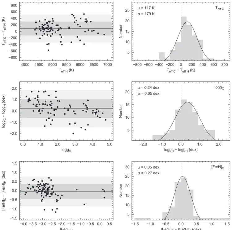
Figure 2 illustrates comparisons of TeffC, log gC, and [Fe/H]Cfor our program stars with the adopted high-resolution results. Note that, with the exception of a few individual stars lying outside the 2σ bands shown on the left panels, their agreement is quite satisfactory. Maximum-likelihoodfits to the distributions of residuals between these various estimates are shown on the right panels. Both the mean offsets(ΔTeffC= 117K, Δlog gC=0.34 dex, Δ[Fe/H]C=0.05 dex) and the scatter in the estimates(σTeffC= 179K, σlog gC=0.65 dex, σ[Fe/H]C=0.27 dex) are reasonably small. Taking into account the expected errors in the high-resolution estimates of these parameters (125K, 0.4 dex, and 0.2 dex, respectively), we conclude that the external precision of the n-SSPP estimates of TeffC, log gC, and[Fe/H]Cis on the order of 125K, 0.5dex, and 0.2dex, respectively.

Figure 3 shows that a comparison with the (non-suspect) RAVE determinations is significantly worse for TeffC but commensurate with the comparisons to the high-resolution results for log gC and [Fe/H]C. There are too few stars in common between the stars with RAVE parameter estimates and those with high-resolution estimates to make meaningful comparisons.

Beers et al. (2014) also used literature values of [C/Fe],

based on high-resolution spectroscopic analyses, to derive corrections for the n-SSPP estimates of[C/Fe], as follows:

= - - +

C FeC C FeS 0.068 C FeS 0.273 . 4

[ ] [ ] ( · [ ] ) ( )

The corrected values are listed as [C/Fe]C in column (8) of Table3. This table also lists, in column(9), the absolute value of the carbon abundance, A(C) = logò (C).11 We assume, following Beers et al., that external errors for [C/Fe]C are on the order of∼0.20 dex.

The parameter CEMP, shown in column (10) of Table 3, indicates whether the star is considered carbon enhanced (CEMP=“C,” satisfying [C Fe]C > +0.7, CC0.7, and



EQW 1.2), of intermediate carbon enrichment (CEMP= “I,” satisfying +0.5<[C Fe]C +0.7, CC0.7, and



EQW 1.2), or carbon normal (CEMP=“N,” satisfying  +

C FeC 0.5

[ ] , CC +0.7, and EQW1.2). Stars with upper limits on their carbon ratios are indicated by CEMP=“U” (these include stars with DETECT=“U,”

 +

CC 0.7, and DETECT=“D” but CC< +0.7). Stars without carbon measurements are listed as CEMP=“X.” There are 48 stars listed with CEMP=“C,” 29 with CEMP=“I,” 1362 with CEMP=“N,” and 116 with CEMP=“U.”

3.4. Distance Estimates and Proper Motions

Distances to individual stars in our sample are estimated using the MVversus(B-V) relationships described by Beers et al.0

(2000). These relationships require that the likely evolutionary

stage of a star be given. Assignments to the evolutionary stage, based on the derived(corrected) stellar atmospheric parameters, are as follows: dwarf, D log( gC 4.0); turnoff, TO (3.5loggC <4.0); and subgiant or giant,G log( gC <3.5). Note that refinements to this scheme, designed to resolve the possible incorrect assignments of TO stars at cooler tempera-tures, are adopted as described in Beers et al.(2012). Following

Santucci et al. (2015), stars with effective temperature



T effC 6000K and loggC 3.5 are classified as field

horizontal-branch(FHB) stars.

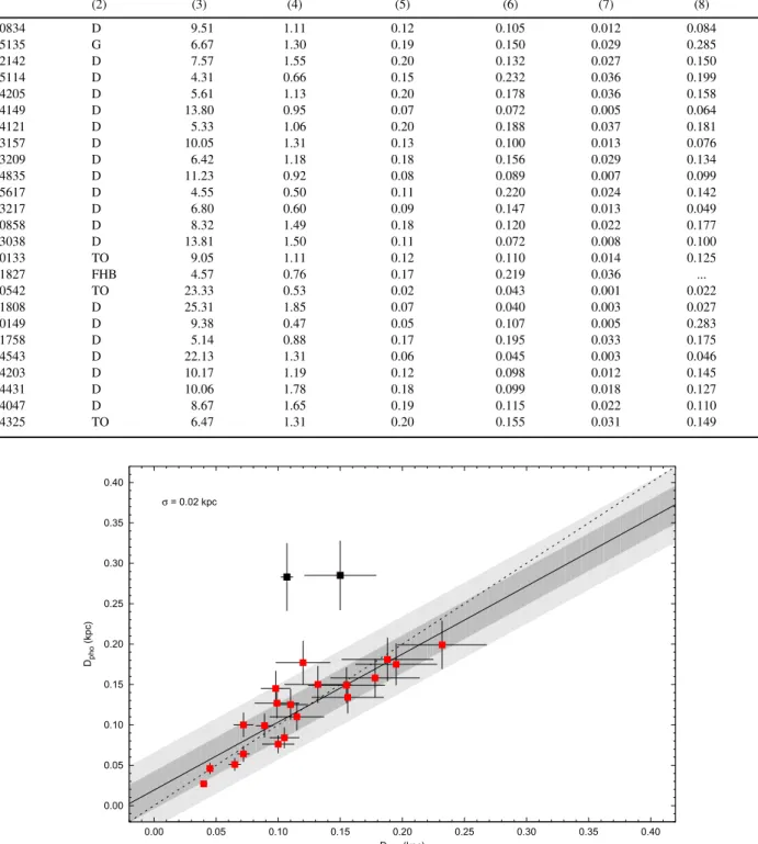
Based on previous tests of this approach, we expect the distances assigned as described above to be accurate on the order of 15%. Fortunately, there are a small number of stars (24) in our sample with reliable distance estimates available from Hipparcos parallax measurements, listed in Table4, using the van Leeuwen (2007) reduction. Column (1) lists the star

names, column(2) the assigned evolutionary type, column (3) the Hipparcos parallax pHIP, column (4) the error on the

parallax spHIP, and column (5) the ratio spHIP pHIP. In order to be

considered a reliable estimate of the parallax, this ratio should be less than 0.20. The parallax distance estimate and its error are listed as DHIPand sDHIPin columns(6) and (7), respectively.

The estimated photometric distances Dphoand their errors sDpho

are provided in columns(8) and (9), respectively.

Figure4presents a comparison of the distances calculated on the basis of the photometric estimates and Hipparcos parallaxes. From inspection of this figure, a great majority of the stars have commensurate distance estimates; the one-sigma scatter of the residuals varies between 10% and 20%, on the order of our adopted distance error of 15%. The most deviant stars include one giant and one dwarf.

11

A(C) is not measured directly—as it can be from high-resolution spectroscopy—but rather obtained from medium-resolution determinations using A(C) = [C/Fe] + [Fe/H] + A(C)e, where we adopt the solar abundance of carbon from Asplund et al.(2009), A(C)e=8.43.

Table5lists star names in column(1) and the assigned type classifications, photometric distance estimates, and their errors in columns(2)–(4), respectively.

The great majority of our program stars (1732 stars) have reasonably high-quality proper motions available from the UCAC4 catalog (Zacharias et al. 2013), the SPM4 catalog

(Girard et al. 2011; 321 stars), or the Hipparcos (van Leeuwen 2007) and TychoII catalogs (Høg et al. 2000; 66 stars). We have chosen to adopt, where possible, the UCAC4 proper motions, since they exist for almost all of our stars and generally have very small errors. The only

exception is that when proper motions are available from the Hipparcos or Tycho II catalogs, we adopt those. The final results are listed as ma and md for the proper motions in the R.A. and decl. directions, respectively, in columns (5) and (6) of Table 5. Their associated errors are listed in columns (7) and (8). The source of the adopted proper motion is listed in column(9). Note that, for a small number of stars for which some ambiguity exists as to which star of a listed pair is the one intended(generally those with “A,” “B,” or“F” appended to their names), we do not adopt any proper motions.

Figure 2. Left panels: differences between the (corrected) atmospheric parameters determined by the n-SSPP—TeffC, log gC, and[Fe/H]C—and the values from analyses of high-resolution spectroscopy—TeffH, log gH, and[Fe/H]H—reported in the literature, as a function of the high-resolution spectroscopic values. Filled symbols refer to the program stars. The horizontal solid line is the average of the residuals, while the darker and lighter shaded areas represent the 1σ and 2σ regions, respectively. Right panels: histograms of the residuals between the corrected n-SSPP and high-resolution parameters shown on the left panels. Each panel also lists the average offset and scatter determined from a Gaussianfit.

8

4. A KINEMATIC ANALYSIS OF THE COMBINED FREBEL ET AL.(2006) AND BEERS ET AL. (2014)

SAMPLES

In this section we examine the kinematic properties of our program stars, in combination with a similar local sample of stars originally identified by Bidelman & MacConnell (1973)

and discussed by Beers et al. (2014). The stellar parameter

estimates and derived kinematic quantities of this latter sample were determined in a manner essentially identical to that for our program stars, and they supplement the numbers of stars with lower metallicity for our subsequent analysis. The corrections

to the n-SSPP-derived atmospheric parameter estimates and [C/Fe] for our program stars are identical to those used by Beers et al.(2014). For simplicity, we drop the “C” subscript

on the corrected stellar atmospheric parameters and the carbonicity estimates in the analysis that follows, although it is understood that these are the quantities we have adopted.

Figure5 shows the distribution of the absorption-corrected V0 magnitudes, de-reddened (B-V)0 colors, distance

esti-mates Dpho, and estimates of metallicities [Fe/H] for our

program stars from Paper I. As is immediately clear from inspection of thisfigure, this is a very local sample of stars,

Figure 3. Left panels: Differences between the (corrected) atmospheric parameters determined by the n-SSPP—TeffC, log gC, and[Fe/H]C—and the values from RAVE—TeffR, log gR, and[Fe/H]R—reported in the literature, as a function of the RAVE spectroscopic values. Filled symbols refer to the program stars. The horizontal solid line is the average of the residuals, while the darker and lighter shaded areas represent the 1σ and 2σ regions, respectively. Right panels: Histograms of the residuals between the corrected n-SSPP and high-resolution parameters shown on the left panels. Each panel also lists the average offset and scatter determined from a Gaussianfit.

∼90% of which are located within 0.5 kpc of the Sun. Although the majority of the sample stars have metallicities close to Solar, some 20%(351 stars) of the stars with available metallicity estimates have [Fe H] -0.5, 14% (248 stars) have[Fe H] -1.0, 12% (213 stars) have[Fe H] -1.5, and 10% (171 stars) have[Fe H] -2.0. Figure 6 of Beers et al.(2014) shows similar information for that sample. As can

be appreciated from inspection of thatfigure, these stars include a larger fraction of giants, which explore slightly farther from the Sun, up to 2 kpc(although ∼90% are within 1 kpc of the Sun). Unlike the PaperIstars, almost half of the supplemental

sample(145 stars) have[Fe H] -1.0;there are also 36 stars with [Fe H] -2.0, which makes them useful for our exploration of metal-poor populations of the Galaxy.

Table 4

Parallaxes and Distance Estimates for Stars with Hipparcos Measurements

Star Name Type πHIP spHIP spHIP pHIP DHIP sDHIP Dpho sDpho

(mas) (mas) (kpc) (kpc) (kpc) (kpc) (1) (2) (3) (4) (5) (6) (7) (8) (9) HE0035-0834 D 9.51 1.11 0.12 0.105 0.012 0.084 0.013 HE0115-5135 G 6.67 1.30 0.19 0.150 0.029 0.285 0.043 HE0134-2142 D 7.57 1.55 0.20 0.132 0.027 0.150 0.023 HE0246-5114 D 4.31 0.66 0.15 0.232 0.036 0.199 0.030 HE0422-4205 D 5.61 1.13 0.20 0.178 0.036 0.158 0.024 HE0429-4149 D 13.80 0.95 0.07 0.072 0.005 0.064 0.010 HE0435-4121 D 5.33 1.06 0.20 0.188 0.037 0.181 0.027 HE0455-3157 D 10.05 1.31 0.13 0.100 0.013 0.076 0.011 HE0457-3209 D 6.42 1.18 0.18 0.156 0.029 0.134 0.020 HE0511-4835 D 11.23 0.92 0.08 0.089 0.007 0.099 0.015 HE0520-5617 D 4.55 0.50 0.11 0.220 0.024 0.142 0.021 HE1108-3217 D 6.80 0.60 0.09 0.147 0.013 0.049 0.007 HE1120-0858 D 8.32 1.49 0.18 0.120 0.022 0.177 0.027 HE1211-3038 D 13.81 1.50 0.11 0.072 0.008 0.100 0.015 HE1223-0133 TO 9.05 1.11 0.12 0.110 0.014 0.125 0.019 HE1349-1827 FHB 4.57 0.76 0.17 0.219 0.036 ... ... HE1411-0542 TO 23.33 0.53 0.02 0.043 0.001 0.022 0.003 HE1450-1808 D 25.31 1.85 0.07 0.040 0.003 0.027 0.004 HE2231-0149 D 9.38 0.47 0.05 0.107 0.005 0.283 0.042 HE2255-1758 D 5.14 0.88 0.17 0.195 0.033 0.175 0.026 HE2307-4543 D 22.13 1.31 0.06 0.045 0.003 0.046 0.007 HE2327-4203 D 10.17 1.19 0.12 0.098 0.012 0.145 0.022 HE2332-4431 D 10.06 1.78 0.18 0.099 0.018 0.127 0.019 HE2333-4047 D 8.67 1.65 0.19 0.115 0.022 0.110 0.017 HE2333-4325 TO 6.47 1.31 0.20 0.155 0.031 0.149 0.022

Figure 4. Comparison of the photometrically estimated distances Dphowith the trigonometric distance estimates DHIPfor stars with sufficiently accurate Hipparcos parallaxes(spHIPpHIP0.20). The dashed line is the one-to-one line, while the solid line is a robust regression fit to the data. The darker and lighter shaded areas represent the 1σ and 2σ regions about the linear fit, respectively, based on a Gaussian fit to the residuals. The most deviant stars include one giant and one dwarf.

10

4.1. Determination of U, V, and W Velocity Components and Orbital Eccentricities for the Frebel et al.(2006) Sample The derivation of space motions and orbital parameters of our program stars from Paper Ifollows the procedures

described by Carollo et al.(2010), which for convenience are

summarized below. Similar procedures were employed by Beers et al.(2014) for the supplemental stars; results are listed

in Table 5 of that paper.

Corrections for solar motion with respect to the local standard of rest (LSR) are applied during the course of the calculation of the full space motions; here we adopt the values (U, V, W)=(9, 12, 7) km s−1 _{(Mihalas & Binney1981). We} follow the convention that U is positive in the direction away from the Galactic center, V is positive in the direction of Galactic rotation, and W is positive toward the north Galactic pole. It is also convenient to obtain the rotational component of a starʼs motion about the Galactic center in a cylindrical frame, denoted as Vf and calculated assuming that the LSR is in a circular orbit with a value of 220 km s−1 (Kerr & Lynden-Bell 1986). Our assumed values of the solar radius

(R=8.5 kpc) and the circular velocity of the LSR are both

consistent with two recent independent determinations of these quantities by Ghez et al. (2008) and Koposov et al. (2009).

Bovy et al. (2012) obtained an estimate of the Milky Wayʼs

circular velocity at the position of the Sun of Vc(R) =

218±6 km s−1, based on an analysis of high-resolution spectroscopic determinations from APOGEE, which is also consistent with our adopted value.

The orbital parameters of the stars, including the perigalactic distance rperi(the closest approach of an orbit to the Galactic

center), the apogalactic distance rapo of each stellar orbit (the

farthest extent of an orbit from the Galactic center), and the orbital eccentricity e = (rapo−rperi)/(rapo+rperi), as well as Zmax (the maximum distance that a stellar orbit achieves above

or below the Galactic plane), are derived by adopting an analytic Stäckel-type gravitational potential(which consists of a flattened, oblate disk and a nearly spherical massive dark-matter halo; see the description given by Chiba & Beers2000, Appendix A) and integrating their orbital paths based on the starting point obtained from the observations.

Table 6 provides a summary of the above calculations. Column(1) provides the star names. Columns (2) and (3) list the positions of the stars in the meridional (R, Z)-plane. The derived U, V, and W velocity components are provided in columns (4)–(6); their associated errors are listed in columns (7)–(9). Column (10) lists the velocity projected onto the Galactic plane (VR, positive in the direction away from the Galactic center), while column (11) lists the derived rotation velocityV . The derived rf periand rapoare given in columns(12)

and (13), respectively. Columns (14) and (15) list the derived

Zmax and orbital eccentricity e, respectively. The INOUT

parameter listed in column (16) is set to 1 if the star is considered in our kinematic analysis, and set to 0 if not.

Errors on our derived estimates of the individual components of the space motions take into account an estimated 15% error in the photometric distances, as well as the individual errors in the proper motions(the average error on our adopted proper motions is 1.3 mas yr−1 in each of the R.A. and decl. component directions) and in the adopted radial velocities (2 km s−1 _{for the high-resolution determinations, 5 km s}−1_for the moderate-resolution determinations, and 10 km s−1for the medium-resolution determinations). Figure 6 shows the distributions of these errors. After removing the 145 stars that are missing one or more of the input quantities used for the determination of their space motions or have individual estimated errors larger than 50 km s−1in any one of the three components of space motion, we obtain for our program sample average errors of s U V W( , , )= (5.9, 6.3, 6.9) km s−1.

Table 5

Distance Estimates and Proper Motions

Star Name Type Dpho sDpho μα μδ sma smd PM Source

(kpc) (kpc) (mas yr−1_{) (mas yr}−1_{) (mas yr}−1_{) (mas yr}−1₎

(1) (2) (3) (4) (5) (6) (7) (8) (9) HE0000-3017 D 0.249 0.037 20.0 1.3 1.1 0.8 U HE0000-4401 D 0.174 0.026 23.6 11.5 1.0 2.9 U HE0000-5703 D 0.253 0.038 13.9 2.6 0.9 1.0 U HE0001-4157 D 0.107 0.016 −19.9 −54.8 0.8 0.8 U HE0001-4449 TO 0.223 0.033 −1.0 0.7 1.1 1.0 U HE0001-5640 D 0.249 0.037 40.2 −13.0 1.0 1.2 U HE0002-3233 TO 0.430 0.065 57.4 −31.6 1.3 1.5 U HE0002-3822 D 0.158 0.024 −36.2 −8.9 1.0 1.5 U HE0002-5625 D 0.258 0.039 11.8 −4.9 1.4 1.4 U HE0003-0503 G 0.163 0.024 9.5 −1.5 1.8 1.3 U

Note. Sources of proper motions: U = UCAC4, S = SPM4, H = Hipparcos or Tycho II. (This table is available in its entirety in machine-readable form.)

Figure 5. Distributions of (a) absorption-corrected V0 magnitudes,(b) de-reddened (B-V) colors,0 (c) photometric distance estimates Dpho, and(d) metallicity estimates[Fe/H] for our program stars.

Table 6

Space Motions and Orbital Parameters

Star Name R Z U V W σ(U) σ(V ) σ(W) VR Vf rperi rapo Zmax e INOUT

(kpc) (kpc) (kms−1_{) (kms}−1_{) (kms}−1_{) (kms}−1_{) (kms}−1_{) (kms}−1_{) (kms}−1_{) (kms}−1_{) (kpc) (kpc) (kpc)} (1) (2) (3) (4) (5) (6) (7) (8) (9) (10) (11) (12) (13) (14) (15) (16) HE0000-3017 8.454 −0.244 8 4 −19 4 2 10 9 224 8.30 8.82 0.36 0.03 1 HE0000-4401 8.450 −0.164 12 12 3 4 2 5 12 232 8.34 9.32 0.18 0.06 1 HE0000-5703 8.407 −0.217 −3 −2 −20 3 2 4 −6 218 8.10 8.47 0.34 0.02 1 HE0001-4157 8.471 −0.102 −26 −6 26 3 3 5 −27 213 7.50 8.99 0.35 0.09 1 HE0001-4449 8.436 −0.210 −7 15 16 2 1 5 −8 235 8.39 9.51 0.32 0.06 1 HE0001-5640 8.410 −0.215 32 −17 18 7 6 9 30 203 6.90 8.81 0.33 0.12 1 HE0002-3233 8.417 −0.422 52 −98 −68 12 17 10 52 122 3.54 8.84 1.61 0.43 1 HE0002-3822 8.462 −0.153 −34 19 21 5 2 10 −34 239 8.04 10.45 0.35 0.13 1 HE0002-5625 8.407 −0.223 −6 −7 −12 4 4 9 −9 213 7.72 8.48 0.27 0.05 1 HE0003-0503 8.506 −0.148 −2 22 −26 2 2 5 0 242 8.51 10.19 0.43 0.09 1

Note. INOUT takes on a value of “1” if the star is accepted for the kinematic analysis, or “0” if not. (This table is available in its entirety in machine-readable form.)

12 The Astrophysical Journal, 835:81 (22pp ), 2017 January 20 Beers et al.

These are slightly smaller errors than were acquired (after the removal of stars having errors in U, V, or W greater than 50 km s−1) for the supplemental stars from Beers et al. (2014),

who reported s U V W( , , )= (7.9, 9.1, 6.5) km s−1, presumably due to the inclusion of more distant stars with less certain distances and proper motions.

For the remaining analysis, we combine our program stars from PaperIwith the supplemental sample based on the Beers

et al.(2014) analysis of the “weak metal” stars from Bidelman

& MacConnell (1973). For the purpose of the kinematic

analysis, both samples have had stars with errors in excess of 50 km s−1in any of the U V W, , velocity componentsremoved from consideration.

4.2. Distributions of U, V, W, and Zmax versus[Fe/H]

Figure 7 presents the individual components of the space motions as a function of[Fe/H] for our combined sample with accepted kinematic estimates; the program stars from Paper Iare shown as black dots, while the supplemental Figure 6. Errors in the estimation of the local velocity components of the space

motions for the PaperIstars. The vertical dashed lines at 50 km s−1indicate the maximum individual errors allowed for a given star to be included in the subsequent kinematic analysis. The legends provide the mean errors for the accepted stars.

Figure 7. Local velocity components for the combined sample of PaperIstars

(shown as black dots) and the supplemental stars from Beers et al. (2014)

(shown as red squares) with available UVW estimates, as a function of metallicity[Fe/H]. Note the existence of stars with low velocity dispersions in their estimated components down to at least[Fe/H] = −1.3 (possibly a little lower). Stars with errors exceeding 50 km s−1in any of the individual derived components of motion are excluded.

Figure 8. Distribution of Zmax,the largest distance above or below the Galactic plane achieved by a star during the course of its orbit, as a function of metallicity[Fe/H] for the combined sample of PaperIstars (shown as black

dots) and supplemental stars from Beers et al. (2014; shown as red squares). The marginal distributions of each variable are shown as histograms. The horizontal dashed line provides a reference at 3 kpc. Very few stars with metallicity[Fe H]> -1.5achieve orbits that reach higher than this location. Note the logarithmic scale for Zmax.Stars with errorsexceeding 50 km s−1in any of the individual derived components of motion are excluded.

Figure 9. Distribution of metallicity [Fe/H] for the combined sample of stars as a function of derived orbital eccentricity. Stars with errorsexceeding 50 km s−1in any of the individual derived components of motion are excluded.

sample stars are indicated as red squares. From inspection of this figure, the two samples cover similar ranges of [Fe/H], although in different proportions—the Paper Isample

dom-inates above [Fe/H] = −1.0, the supplemental sample stars exceed the Paper Istars in the metallicity interval

-2.0<[Fe H]< -1.0 by about a factor of two, and the Paper Istars dominate the combined sample of stars with

< -Fe H 2.0

[ ] , in particular for [Fe H]< -3.0. The com-bined sample is heavily populated by stars in the thin-disk and thick-disk stellar populations. Some low-metallicity stars with V velocities in the interval−40 to −80 km s−1are also present and are likely to be associated with the MWTD.

Figure 8 is a plot of Zmax as a function of[Fe/H] for the

combined sample of stars. From inspection of this figure, it is clear that both the Paper Iand supplemental samples explore

similar regions of this space, further justifying a joint kinematic analysis. For the remainder of our analysis, we thus choose to suppress identification of the individual samples.

As seen in Figure8, only a handful of stars with metallicities above [Fe/H] = −1.5 are found to have Zmax>3 kpc.

Following previous results from, e.g., Carollo et al. (2010),

stars with Zmax „ 3 kpc and -1.8[Fe H]-0.8 are

likely to be associated with the MWTD, although some overlap with the inner-halo population is not precluded, especially at the low end of this metallicity range. Further interpretation of the nature of the MWTD as an individual component is limited by the relatively small numbers of stars, even in the combined sample, that are available in the pertinent metallicity interval.

4.3. The[Fe/H] versus Eccentricity Diagram

Figure 9 shows a plot of [Fe/H] as a function of orbital eccentricity for the combined sample of stars. As seen previously (e.g., Norris et al. 1985; Chiba & Beers 2000; Carollo et al. 2007, 2010; Beers et al. 2014), the orbital

eccentricity for these non-kinematically selected stars exhibits a very broad metallicity distribution, outside of the region of the

metal-richest stars with e0.2 0.3– , as expected from the currently favored hierarchical assembly model for the forma-tion of the Milky Way.

4.4. The Toomre Diagram, the Distribution ofV , Integrals off Motion, and the Lindblad Diagram

The so-called Toomre diagram(a plot of (U2+W2 1 2_{) , the}

quadratic addition of the U and W velocity components as a function of the rotational component V), the distribution of orbital rotation velocityV for cuts in orbital eccentricity andf [Fe/H], plots of the perpendicular angular momentum comp-onent L^ as a function of the vertical angular momentum component LZ, and the Lindblad diagram(a plot of the integral of motion representing the total energy E as a function of LZ) are commonly used to investigate the nature of the kinematics of stellar populations in the Galaxy. Given the high quality of the estimated kinematics for our combined sample of stars, it is worthwhile to investigate what can be learned from inspection of these diagrams, as discussed individually below.

4.4.1. The Toomre Diagram

Figure10shows the Toomre diagram for the combined sample of stars; the legend indicates the metallicity intervals chosen to roughly separate stars expected to belong to the thick(or thin) disk ([Fe H]> -0.8), the MWTD (-1.8<[Fe H]-0.8), and the halo system ([Fe H] -1.8) in accordance with Carollo et al. (2010). As expected, the more metal-rich stars in both

samples are primarily found in the region with low(U2+W2 1 2₎

and high orbital rotation velocities,₍U2+W2 1 2₎ 100_{km s}−1 and -100<V<50 km s−1, while stars with intermediate metallicities are divided between those inside and outside this region. We expect that many of the intermediate-metallicity stars inside this region are associated with the MWTD component. It is also clear from inspection of thisfigure that the lowest-metallicity stars, with[Fe H] -1.8, are the dominant contributors to the distribution of stars in the higher-energy regions(those beyond the circle that intersects V=−300 km s−1), as might be expected if they are primarily comprised of members of the outer-halo population, with some overlap from members of the inner-halo population. The stars with energies that place them between the V=−300 km s−1 and V=−200 km s−1 surfaces exhibit a broader range of metallicity, as expected from overlapping inner-and outer-halo populations.

Figure 10 also indicates two subsets of (newly identified) stars in the combined sample that may belong to previously identified structures in phase-space: (1) likely members of the stream/trail of stars first identified by Helmi et al. (1999) and

further populated by stars in the sample considered by Chiba & Beers(2000), indicated by light-green squares, and (2) possible

members of the debris stream associated with the globular clusterω Cen, following the work of Dinescu (2002), Klement

et al. (2009), and Majewski et al. (2012), indicated by

light-blue circles. Justification for the selection of these stars is provided below.

4.4.2. Distribution ofVf

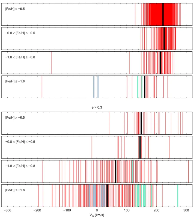
Figure11is a stripe-density diagram of the distribution ofVf for our combined sample of stars for metallicity intervals chosen to emphasize the various kinematic components of the Milky Way, split into two regions of orbital eccentricity,



e 0.3(upper panels, expected to be dominated by members

Figure 10. Toomre diagram of (U2+W2 1 2_{) vs. V for stars in the combined} sample with available UVW velocity components, in three regimes of metallicity as indicated in the legend. The legend also indicates the color/ symbol coding used to indicate likely members of stars in the debris stream associated with the globular clusterω Cen (light-blue circles) and the Helmi et al. stream/trail (light-green squares). See text for more details. Note the presence of intermediate-metallicity (-1.8<[Fe H]-0.8) stars both inside and outside the region with low(U2+W2 1 2_{) and high orbital rotation} velocities ((U2+W2 1 2₎ 100_{km s}−1_{, -100<V<100 km s}−1_{). Stars} with errorsexceeding 50 km s−1in any of the individual derived components of motion are excluded.

14

of the disk system) and >e 0.3(lower panels, expected to be dominated by members of the halo system). For each interval in metallicity, the black stripes indicate the meanV for that sub-f sample of stars. The light-green and light-blue stripes indicate stars that we argue below are candidate members of the Helmi et al. stream/trail and the ω Cen debris streams, respectively.

Inspection of Figure11generally meets expectation based on previous work. The low-eccentricity stars for all three sub-panels with [Fe H]> -1.8 exhibit rotational properties consistent with those of the disk system of the Milky Way (thin disk, thick disk, and MWTD), while those with

 -Fe H 1.8

[ ] appear to be primarily members of the inner-and outer-halo populations. The high-eccentricity stars prefer-entially populate the sub-panels with-1.8<[Fe H]-0.8 and[Fe H] -1.8, consistent with membership in the inner-and outer-halo populations, with overlapping contributions from each.

It is worth noting that the presence of putative members of the two debris streams has a potentially large impact on interpretation of the distribution of Vf among the high-eccentricity stars with [Fe H]< -1.8, with these members populating both the central region of the stripe plot(the Helmi

Figure 11. Stripe-density diagrams of the rotational velocityV for stars in the combined sample. The plots are split into low-eccentricityf ( e 0.3; upper panels) and high-eccentricity( >e 0.3; lower panels) sub-samples. Each sub-sample is further divided into metallicity intervals chosen to separate regions dominated by individual components of the disk and halo systems. See text for more details. The black stripes indicate the meanV for the stars in each subset. The light-blue and light-greenf stripes indicate stars identified as likely members of stars in the debris stream associated with the globular cluster ω Cen and the Helmi et al. stream/trail, respectively. Stars with errors exceeding 50 km s−1in any of the individual derived components of motion are excluded.

et al. stream/trail) and the high-velocity tail (the ω Cen debris stream).

4.4.3. L_⊥versus LZ

The left panel of Figure12shows the distribution of stars in angular momentum space(L⊥, LZ), where L⊥=(LX2+LY2) and LZis the vertical angular momentum. The three different ranges of metallicity are identified with different colors, shown in the figure legend.

Two interesting features are seen in this diagram: (1) a clump of stars with[Fe H]< -1.8 (with the exception of two stars with higher metallicity) located at L⊥∼2000– 2900 kpc km s−1 and LZ∼800–1600 kpc km s−1 (indicated by the solid black box in the figure) and (2) an elongated distribution of stars with [Fe H] -1.8 located at L_⊥>1500 km s−1 and −400LZ300 kpc km s−1 (indi-cated by the orange box).

The first feature was identified by Helmi et al. (1999),

comprising 7 stars with [Fe H] -1.6 and 12 stars with 

-Fe H 1.0

[ ] . Chiba & Beers(2000) detected the same stream

among their sample of 1203 stars over similar ranges in metallicity. They also identified a possible trail in angular momentum space located at 1250 kpc km s−1<L_⊥<2000 kpc km s−1 and 1200 kpc km s−1 < LZ<2000 kpc km s−1 and covering similar metallicity ranges (their Figure 15). This is similar to the trail identified in Figure12, occupying the region defined by the dotted black box and covering angular momentum ranges of L_⊥= [1300, 2000] kpc km s−1 and LZ = [1000, 1600] kpc km s−1, but at lower metallicities[Fe H] -1.8. Note that a few stars with metallicities above [Fe/H]=−1.8 are also within the areas delimited by the two boxes associated with the Helmi et al. stream/trail.

The second feature(orange box) is similar to the excess of stars located in the phase-space noted by Dinescu(2002) within

the Chiba & Beers (2000) data set. Dinescu argued that these

stars may be part of a debris stream associated with the globular

clusterω Cen. Dinescu (2002) found that most of the stars in

this region possessed slightly retrograde orbits, as is also the case forω Cen, and discovered another two clusters (NGC362 and NGC6779) that present similar retrograde orbits. The author also suggested that the clusterω Cen (shown as a large orange star in the figure), as well as the two other globular clusters, may have been stripped, along with numerous other stars, from a proposed parent dwarf galaxy now dissolved into the halo-system population.

4.4.4. The Lindblad Diagram, E versus LZ

The right panel of Figure 12 is the so-called Lindblad diagram for the combined sample, split into the same metallicity ranges as on the left panel. Stars associated with the Helmi et al. (1999) stream and its trail are indicated with

light-green boxes around them, while those identified as possible members of the ω Cen debris stream are indicated with light-blue circles around them. The Helmi et al. stream and its trail occupy a range of orbital energy E = [−1.2, −0.7] km2_s2_{(in units of 10}5_{), while the putative ω Cen stellar} debris stream stars have orbital energies spanning E: [−1.35, −0.8] km2_s2_.

The stars we identify as members of these structures are listed in column (1) of Table 7, along with their coordinates (column 2), photometry (columns 3 and 4), derived metallicity [Fe/H] (column 5), carbonicity [C/Fe] (column 6), and absolute carbon abundance A(C) (column 7), as well as their integrals of motion(columns 9–11). We have verified that these stars are not among those previously identified by Chiba & Beers(2000). There are five CEMP stars among the proposed ω

Cen debris stream listed in this table, with carbonicities in the range [C/Fe] = [+0.73, +1.47]. The listed absolute carbon abundances for four of these stars, A(C), are all below 7.1; according to the Yoon–Beers diagram of A(C) versus [Fe/H] (Yoon et al. 2016; Figure 1), they would be classified as CEMP-no stars. There is one star in the proposedω Cen debris

Figure 12. Left panel: distribution of the angular momentum componentsL and L^ Zfor the combined sample of stars over three ranges of metallicity, as shown in the legend. The solid and dotted black boxes denote the region of the clumps that are likely associated with the Helmi et al. stream and trail, respectively. The orange box represents the region of the putative debris stream associated with theω Cen globular cluster. The position of this cluster in this diagram is indicated by the large orange star. Stars with errors exceeding 50 km s−1 in any of the individual derived components of motion are excluded. Right panel: Lindblad diagram of the distribution of the total energy E(in units of 105_{) as a function of the vertical angular momentum L}

Zover three ranges of metallicity, as shown in the legend. Likely members of the Helmi et al. stream and its trail are highlighted with light-blue circles; stars that are likely members of the putativeω Cen debris stream are indicated by light-green squares. The position of this cluster in this diagram is indicated by the large orange star. Stars with errors exceeding 50 km s−1in any of the individual derived components of motion are excluded.

16

stream with A(C)>7.1, which would suggest its identification as a CEMP-s star. The CEMP sub-classifications are shown in column (8) of Table7.

In a previous study, Majewski et al. (2012) identified a

number of carbon-enhanced stars from the Grid Giant Stream Survey sample that may be associated with the purportedω Cen debris stream. Many of these stars exhibit enhanced [Ba/Fe]

Table 7

Parameters for Stars in the Identified Streams

Star Name R.A.(2000) Decl. V B−V [Fe/H]C [C/Fe]C A(C) Class L⊥ LZ E (mag) (mag) (kpc km s−1_{) (kpc km s}−1_{) (10}5_km2_s−2₎

(1) (2) (3) (4) (5) (6) (7) (8) (9) (10) (11)

Helmi et al. Debris Stream

HE0012-5643a 00 15 17.1−56 26 27 12.29 0.46 −2.97 +1.41 6.87 CEMP-s 2466 1132 −0.81 HE0017-3646 00 20 26.1−36 30 20 13.02 0.54 −2.48 −0.54 5.41 ... 2729 1169 −0.92 HE0048-1109a 00 51 26.4−10 53 14 10.83 0.49 −1.97 −0.10 6.36 ... 2187 1337 −1.07 BM-028 02 47 37.4−36 06 27 9.94 0.46 −1.58 +0.24 7.31 ... 2259 1020 −1.11 HE0324-0122 03 27 02.3+01 32 33 12.13 0.72 −2.11 +0.37 6.69 ... 2311 1493 −1.06 BM-209 14 36 48.5−29 06 47 8.02 0.64 −1.91 +0.06 6.66 ... 2152 1146 −1.14 HE2215-3842 22 18 20.9−38 27 55 13.40 0.68 −2.24 +0.45 6.64 ... 2062 1093 −0.97 BM-308 22 37 08.1−40 30 39 9.11 0.79 −2.12 −0.10 6.39 ... 2313 1124 −0.73

Helmi et al. Trail

HE0033-2141a _{00 35 42.1−21 24 58 12.29 0.72 −2.73 +0.15 5.85 ... 1407 1559 −1.11} HE0050-0918 00 52 41.7−09 02 23 11.06 0.71 −2.08 −0.26 6.09 ... 1653 1122 −1.14 HE1210-2729a _{12 13 07.9−27 45 50 12.54 0.86 −2.95 −0.18 5.31 ... 1589 1172 −1.09} BM-235 17 52 35.9−69 01 45 9.48 1.05 −1.83 −0.44 6.39 ... 1925 1130 −1.17 HE2234-4757a _{22 37 20.4−47 41 38 12.39 0.92 −2.59 −0.26 5.57 ... 1455 1441 −1.10}

ω Cen Debris Stream

HE0007-1752a _{00 10 17.6−17 35 38 11.54 0.65 −2.47 +0.54 6.50 ... 2333 33 −1.17} HE0039-0216a _{00 41 53.6−02 00 33 13.35 0.37 −2.62 +1.40 7.21 CEMP-s 2993 230 −0.93} HE0429-4620 04 30 48.6−46 13 53 13.10 0.62 −2.42 +0.58 6.59 ... 1912 −236 −1.14 HE1120-0153a 04 38 55.7−13 20 48 11.68 0.44 −2.39 −0.17 5.89 ... 2023 140 −0.97 BM-056 05 10 49.6−37 49 03 9.50 0.86 −2.00 −0.16 7.62 ... 2377 −102 −1.12 BM-121a 09 53 39.2−22 50 08 9.39 1.16 −2.69 −0.53 5.65 ... 1550 −84 −1.37 HE1120-0153a 11 22 43.2−02 09 36 11.68 0.44 −2.88 +1.09 6.64 CEMP-no 1569 −41 −1.12 HE1401-0010a 14 04 03.4−00 24 25 13.51 0.41 −2.44 +0.73 6.72 CEMP-no 2681 138 −0.79 HE2138-0314a 21 40 41.5−03 01 17 13.23 0.57 −3.07 +0.90 6.27 CEMP-no 2138 −70 −1.13 HE2315-4306 23 18 19.0−42 50 27 11.28 0.65 −2.36 +0.37 6.43 ... 1712 −202 −1.33 HE2319-5228a 23 21 58.1−52 11 43 13.25 0.90 −3.39 +1.47 6.51 CEMP-no 2170 114 −1.07 HE2322-6125a 23 25 34.6−61 09 10 12.47 0.63 −2.50 +0.17 6.10 ... 2145 −80 −1.20 Note. a

A high-resolution spectrum exists for this star.

Figure 13. Carbonicity [C/Fe] as a function of metallicity [Fe/H] for the combined sample of stars with available measurements. Downward arrows indicate the derived upper limits for[C/Fe], and upward arrows indicate the lower limits. The marginal distributions of each variable are shown as histograms. The horizontal dashed line marks the level of carbon enhancement used in this paper to indicate CEMP stars,[C Fe]> +0.7.

Figure 14. Cumulative frequencies of CEMP stars as a function of metallicity [Fe/H] for stars in the combined sample with available measurements. A total of 328 stars with[Fe H]< -1.0are included in this diagram, 52 of which are considered CEMP stars, with[C Fe]> +0.7. The error bars shown are based on Poisson statistics.