Sensitivity of European glaciers to precipitation and temperature - two case studies

Sensitivity of European glaciers to precipitation

and temperature

– two case studies

Daniel Steiner&Andreas Pauling&

Samuel U. Nussbaumer&Atle Nesje&

Jürg Luterbacher&Heinz Wanner&Heinz J. Zumbühl

Received: 13 October 2006 / Accepted: 15 January 2008 / Published online: 14 March 2008 # Springer Science + Business Media B.V. 2008

Abstract A nonlinear backpropagation network (BPN) has been trained with high-resolution multiproxy reconstructions of temperature and precipitation (input data) and glacier length variations of the Alpine Lower Grindelwald Glacier, Switzerland (output data). The model was then forced with two regional climate scenarios of temperature and precipitation derived from a probabilistic approach: The first scenario (“no change”) assumes no changes in temperature and precipitation for the 2000–2050 period compared to the 1970–2000 mean. In the second scenario (“combined forcing”) linear warming rates of 0.036–0.054°C per year and changing precipitation rates between−17% and +8% compared to the 1970–2000 mean have been used for the 2000–2050 period. In the first case the Lower Grindelwald Glacier shows a continuous retreat until the 2020s when it reaches an equilibrium followed by a minor advance. For the second scenario a strong and continuous retreat of approximately−30 m/year since the 1990s has been modelled. By processing the used climate parameters with a sensitivity analysis based on neural networks we investigate the relative importance of different climate configurations for the Lower Grindelwald Glacier during four well-documented historical advance (1590– 1610, 1690–1720, 1760–1780, 1810–1820) and retreat periods (1640–1665, 1780–1810, 1860–1880, 1945–1970). It is shown that different combinations of seasonal temperature and

D. Steiner

:

:

:

:

Institute of Geography, Climatology and Meteorology, University of Bern, Hallerstrasse 12, CH-3012 Bern, Switzerland

D. Steiner (*)

:

:

:

Oeschger Centre for Climate Change Research (OCCC) and National Centre of Competence in Research on Climate (NCCR Climate), University of Bern, Erlachstrasse 9a, CH-3012 Bern, Switzerland e-mail: steiner@giub.unibe.ch

A. Nesje

Department of Earth Science, University of Bergen, Allégaten 41, N-5007 Bergen, Norway A. Nesje

Bjerknes Centre for Climate Research, Allégaten 55, N-5007 Bergen, Norway A. Pauling

Federal Office of Meteorology and Climatology, MeteoSwiss, Krähbühlstrasse 58, CH-8044 Zürich, Switzerland

precipitation have led to glacier variations. In a similar manner, we establish the significance of precipitation and temperature for the well-known early eighteenth century advance and the twentieth century retreat of Nigardsbreen, a glacier in western Norway. We show that the maritime Nigardsbreen Glacier is more influenced by winter and/or spring precipitation than the Lower Grindelwald Glacier.

1 Introduction

Primarily motivated by investigations of climate change, the scientific community has become increasingly aware that mountains and their environments are highly sensitive indicators of climate variability over the decadal to centennial timeframe. Particularly mountain glaciers are key variables for early detection strategies in global climate-related observations. Their fluctuations have been observed systematically in various parts of the world since the end of the nineteenth century, and are therefore an impressive manifestation of varying climatic conditions (Haeberli 2006). Corresponding to global trends in temperature, they have retreated significantly since the mid-nineteenth century (e.g. McCarthy et al. 2001; Houghton et al. 2001; Paul et al.2004; Oerlemans2005; Solomon et al.2007).

Today, the World Glacier Monitoring Service WGMS (http://www.geo.unizh.ch/wgms/) collects standardized observations on changes in mass, volume, area and length of glaciers with time (glacier fluctuations), as well as statistical information on the distribution of perennial surface ice in space (glacier inventories). Such glacier fluctuation and inventory data form a basis for better understanding and modelling the climate–glacier relation (Haeberli2006). Many studies have been carried out to investigate the relationship between climatic signals and variations of glaciers. For this purpose, regression techniques have often been used to relate for instance mean mass balance to climatic variables. In these studies the number and type of predictors may differ significantly and depend on what is inferred to influence glacier mass balance (e.g. Oerlemans and Reichert 2000, and references therein). Unfortunately, direct measurements of mass balance are labour-intensive, expensive to maintain and therefore few in number. These records are short and cover only the past few decades (Haeberli2006).

On the other hand some long records of front positions of glaciers in Europe are available. The longest and one of the best-documented record is that of the Lower Grindelwald Glacier which starts in 1535 (Zumbühl1980; Zumbühl et al.1983; Oerlemans 2005). Change in glacier length is an easily measured but indirect, filtered and delayed response of climate change (Oerlemans2001). Nevertheless, it can be used to reconstruct glacier mass balance (Haeberli and Hoelzle1995; Hoelzle et al.2003; Zemp et al.2006) as well as large scale temperature changes over the last centuries (Oerlemans2005).

However, the complexity of available glacier–climate models is as wide as the possible application of such models. The models range from those using air temperature as a sole index for energy available for melt to those that evaluate the surface energy fluxes to great details (e.g. Reichert et al.2001; Nesje and Dahl2003; Klok and Oerlemans2004). Besides these classical methods that commonly use linear assumptions, neural network models (NNMs) have become popular for performing nonlinear regression and classification since the late 1980s. More recently, NNMs have been extended to perform nonlinear principal component and nonlinear canonical correlation analysis (Hsieh2004). However, neural networks (NNs) have acquired a solid position in many fields of human activity. Due to both improvements in the models and to the enormous increase in the quality and quantity of data, they have found application in a large variety of scientific problems, among them environmental sciences (e.g.

Hsieh and Tang1998; see Section2.4for some NN applications), astronomy (Tagliaferri et al. 2003), geophysics (Sandham and Leggett2003) and medicine (Papik et al.1998).

An objective of the present paper is to show the capabilities of nonlinear NNs in a glaciological context. It is also intended to be a follow-up to a first study on this subject (Steiner et al.2005), which proposes a NN method to reconstruct the mass balance series of the Great Aletsch Glacier, Switzerland, back to 1500. That study dealt with monthly and seasonal temperature and precipitation data as driving factors of the glacier model and on a mass balance record as target variable.

Thus, besides the problem of simulating future glacier front variations of the Lower Grindelwald Glacier, a sensitivity analysis of potential climatic influences on two appropriate glaciers, using a NN approach, is discussed here.

In Section2we give an overview of the data used in this study and the concept of the NN approach. As an important example of a NN, we discuss the backpropagation network (BPN). Furthermore, we perform a sensitivity analysis based on a BPN to measure the time-dependent influence of temperature and precipitation on the Lower Grindelwald Glacier, Switzerland, and Nigardsbreen Glacier, Norway.

Section3deals with the simulation of future length variations of the Lower Grindelwald Glacier, Switzerland, by using neural networks. Furthermore, we analyze the sensitivity of glacier variations to seasonal temperature and precipitation, again based on NNs. For an independent comparison we apply this method to Nigardsbreen Glacier, Norway.

In Section 4 the results and the performance of the used methods are discussed. In Section5conclusions are provided and further scientific investigations are proposed.

2 Data and methods

2.1 The study sites

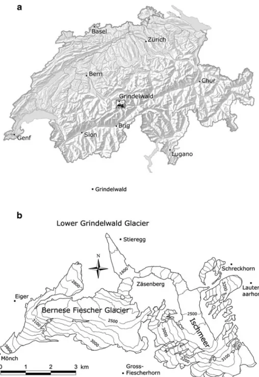
Figure1shows the topography and some locations within the greater region of the Lower Grindelwald Glacier, situated in the northern Bernese Alps (western Switzerland) and the location of the Lower Grindelwald Glacier in Switzerland. Table 1 gives some further characteristics of the Lower Grindelwald Glacier.

The Bernese Alps are one of the main European watersheds, separating the catchment area of the Aare (draining into the North Sea via the Rhine) from that of the Rhône (which flows into the Mediterranean Sea). According to their geographic situation between 46° N and 47° N, the climate of the Bernese Alps is of temperate character, typical for the southern side of the extratropical westerlies. It constitutes a border between the Mediterranean and the North Atlantic climate zone (Wanner et al. 1997). The northern part of the Bernese Alps, shows maximum precipitation during summer, with quite small interannual variability. The mean annual temperature at Grindelwald (1,040 meters asl.), located approximately 3 km from the glacier front of the Lower Grindelwald Glacier, was 6.7°C during the 1966–1989 period. The mean temperature during the accumulation season (October–April) and ablation season (May–September) during the 1966–1989 period was 2.3°C and 12.9°C, respectively. Note that the definitions of the above-mentioned seasons, basing on the hydrological year and atmospheric conditions, are widely used in glaciology (e.g. Schöner and Böhm2007; Rasmussen et al.2007).

The mean annual precipitation at Grindelwald during the 1961–1990 normal period was 1,428 mm. The precipitation during the accumulation season (October–April) and ablation season (May–September) during the 1961–1990 normal period was 720 and 708 mm,

Fig. 1 a The Grindelwald region (area with solid outline) within Switzerland. b Map showing some remarkable locations, mountain peaks and the topography of the Lower Grindelwald Glacier with its main branches and tributaries

respectively (data from the online database of MeteoSwiss). Because of the high precipitation (locally exceeding 4,000 mm/year), the Bernese Alps show a relative low glacier equilibrium line altitude (ELA) and are the mountain range showing the heaviest glacierization of the Alps. Both the glacier with the lowest front (Lower Grindelwald Glacier; this study) and the largest glacier of the Alps (Great Aletsch Glacier; Steiner et al. 2005) are situated within this region (Kirchhofer and Sevruk1992; Imhof1998).

The Nigardsbreen Glacier is an outlet from the largest ice cap in Norway, Jostedalsbreen (487 km2). Figure2a shows the location of the glacier within western Norway. Shown is also a map of the glacier tongue and its foreland, together with dates of the formation of some of the moraines (Fig. 2b). Table1 shows some characteristics of the Nigardsbreen Glacier. It must be noted that Nigardsbreen Glacier has an equilibrium line altitude (ELA) much higher than the deep U-shaped terminus region (Fig.2b) and flat accumulation areas at high altitude. This explains why it currently shows the most positive net balance in Norway (Chinn et al.2005).

The mean annual temperature at Bjørkehaug (324 meters asl.), located approximately 5 km from the glacier front of Nigardsbreen, was 3.7°C during the 1961–1990 normal period. The mean temperature during the accumulation season (October–April) and ablation season (May–September) during the 1961–1990 normal period was −1.4°C and 10.9°C, respectively. The mean annual precipitation during the 1961–1990 normal period was 1,380 mm. The precipitation during the accumulation season (October–April) and ablation season (May–September) during the 1961–1990 normal period was 920 and 460 mm, respectively (data from the Norwegian Meteorological Institute).

2.2 Multiproxy reconstructions of temperature and precipitation back to 1500

Luterbacher et al. (2004) and Xoplaki et al. (2005) reconstructed monthly European surface air temperature patterns back to 1659 and seasonal estimates from 1500–1658 at 0.5°×0.5° resolution. The reconstruction of Luterbacher et al. (2004) is based on a comprehensive data set that includes a large number of homogenized and quality-checked instrumental data series, a number of reconstructed sea-ice and temperature indices derived from documentary records (e.g. Brazdil et al. 2005, for a review) for earlier centuries, and a few seasonally resolved natural proxies from Greenland ice cores and tree rings from Scandinavia and Siberia that resolve seasonal temperature. Documentary evidence comprises all non-instrumental man-made data on past weather and climate as well as instrumental

Table 1 Topographical characteristics of the Lower Grindelwald Glacier, Switzerland (data from 2004: Steiner at al.2008), and Nigardsbreen Glacier, Norway (data from 1986: Østrem et al.1988)

Lower Grindelwald Glacier Nigardsbreen Geographical coordinates 8°05′ E, 46°35′ N 7°08′ E, 61°45′ N

Length (km) 8.85 9.6

Surface area (km2) 20.6 48.2

Elevation of head (meters asl.) 4107 1950

Elevation of terminus (meters asl.) 1297 355

Average height (meters asl.) 2840 1150

Equilibrium line altitude ELA (meters asl.) 2640 1560

Exposure N–NW E–SE

Average slope (%) 31.8 16.6

observations prior to the set-up of continuous meteorological networks. Non-instrumental evidence is subdivided into descriptive documentary data (including weather observations, e.g. reports from chronicles, daily weather reports, travel diaries, ship logbooks, etc.) and documentary proxy data (more indirect evidence that reflects weather events or climatic conditions such as the beginning of agricultural activities, religious ceremonies in favour of ending meteorological stress such as drought or wet conditions, etc.; Brázdil et al.2005).

In comparison to Luterbacher et al. (2004), Xoplaki et al. (2005) used only instrumental temperature series (no station pressure data), adding a few series from Scandinavia, central and eastern Europe, and derived temperature indices from documentary evidence.

Both reconstructions are developed using principal component regression analysis. The leading Empirical Orthogonal Functions (EOFs) of the predictor data variance and the leading EOFs of the total predictand variability (gridded temperature; New et al. 2000; Mitchell and Jones 2005) are calculated for the 1901–1960 calibration period. A

Fig. 2 a Map showing the Jostedalsbreen ice cap with its main branches. b The tongue of the Nigardsbreen Glacier and its foreland with dates of the formation of some of the moraines (Østrem et al.1976). Contour lines are indicated for the years 1937 (dashed lines), 1951 (solid lines) and 1974 (grey lines)

multivariate regression is then performed against each of the grid point EOFs of the calibration period against all the retained EOFs of the predictor data. Applying the multivariate regression model to independent data from the verification period 1961–1995 allows testing the quality of the reconstructions. In a final step, a recalibration over the full calibration and verification period 1901–1995 has been performed in order to derive the final spatial temperature patterns for the period 1500–1900 for the European land areas (see Luterbacher et al.2004, for a detailed description of the reconstruction methods, the used predictor data and the reliability of the reconstructions). Due to the changing number of the predictor data over time, several hundreds of nested models for the 1500–1900 period have been developed for the temperature reconstructions. For this application, the winter and summer temperature estimates of Luterbacher et al. (2004) have been reperformed using a few additional predictor data, excluding station pressure data and fitting to the Mitchell and Jones (2005) data (Luterbacher et al.2007).

Using the same methods as Luterbacher et al. (2004) and Xoplaki et al. (2005) for their temperature reconstructions, Pauling et al. (2006) reconstructed seasonal precipitation back to 1500. That gridded dataset (0.5°×0.5° resolution) covers all Europe (land area only). Three data types are used as predictors: long quality checked instrumental precipitation series, precipitation indices based on documentary evidence and natural proxies (tree-ring chronologies, ice cores, corals and a speleothem) resolving precipitation signals. As in Luterbacher et al. (2004) and Xoplaki et al. (2005) reconstructive skill has been estimated by the Reduction of Error (RE) statistic. In the Pauling et al. (2006) reconstructions, the calibration period was 1901–1956, the period 1957–1983 for verification. The final models that were used for the reconstructions back to 1500 are based on the full 1901–1983 calibration and verification period. For details on the precipitation reconstructions and the spatial skill of the estimated fields, see Pauling et al. (2006).

The reconstructive skill for both the temperature and precipitation reconstructions was estimated to be high for the Grindelwald region. Consequently, for the sensitivity analysis of the Lower Grindelwald Glacier we selected the nearest grid point 8.25° E/46.75° N to the glacier location.

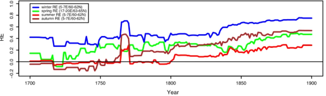
Given the high spatial variability of precipitation it is difficult to skilfully reconstruct precipitation in areas where only sparse predictor information is available due to a lack of precipitation signals of remote regions for such regions. For the Nigardsbreen region the reconstructive skill of the precipitation reconstructions is generally lower than that over central Europe or other parts of Scandinavia (Pauling et al.2006). We therefore averaged the climate reconstructions. For the sensitivity analysis of Nigardsbreen Glacier only two averages of precipitation reconstructions are qualitatively suitable: winter precipitation over 5–7° E/60–62° N (Nigardsbreen area) and spring precipitation over 17–20° E/63–65° N (N-Sweden), the nearest region where reconstructive skill is above zero. The temporal evolution of the RE values is depicted in Fig.3. A problem may arise from the different locations of Nigardsbreen and the reconstructed spring precipitation time series. However, the correlation between spring precipitation in N-Sweden and W-Norway (location of Nigardsbreen Glacier) is highly significant during the twentieth century (p value=0.00013) which suggests that spatial extrapolation over these areas is allowable. Summer and autumn precipitation are omitted due to low reconstructive skill (Pauling et al. 2006). Figure 3also shows the lower data quality of the reconstructions in the first half of the eighteenth century, especially for the summer and autumn precipitation series. Furthermore, it also demonstrates that the RE values may change through time as during different periods different predictors are available. In contrast to the precipitation patterns the

reconstructed temperature data for 5–7° E/60–62° N (Nigardsbreen area) can be considered as reliable (Luterbacher et al.2004).

2.3 Climate scenarios for the Swiss Alpine region

Climate scenarios are plausible representations of future climate that have been constructed for explicit use in investigating the potential impacts of anthropogenic climate change. Climate scenarios often make use of climate projections (descriptions of the modelled response of the climate system to scenarios of greenhouse gas and aerosol concentrations), by manipulating model outputs and combining them with observed climate data (Houghton et al.2001; Solomon et al.2007).

A main problem of climate scenarios are the large uncertainties associated with these model projections, and that uncertainty estimates are often based on expert judgement rather than objective quantitative methods. In a probabilistic approach such uncertainties can be partially quantified from ensembles of climate change integrations, made using different models starting from different initial conditions (Frei2004). For the global mean temperature several probabilistic climate projections have been developed by Wigley and Raper (2001) and Knutti et al. (2002).

Results from regional climate model simulations (Schär et al.2004; Stott et al.2004), under the IPCC SRES A2 transient greenhouse-gas scenario (“business-as-usual”), suggest increasing summer temperatures in central and southern Europe within the twenty-first century with about every second summer that will be as hot or even hotter (or as dry or drier) than 2003 by the end of the twenty-first century (2071–2100).

Frei (2004) performs regional probabilistic projections of temperature and precipitation for the Swiss Alpine region based on simulations with 16 different climate model chains. In this model approach different general circulation models (GCMs) and regional climate models (RCMs) are involved. The IPCC SRES A2 and IPCC SRES B2 ( “dynamics-as-usual”) emission scenarios were used as model inputs. Table 2 shows the two climate scenarios for the 2000–2050 period used in this study. Scenario 1 represents the “no change” climate, i.e. no changes in temperature and precipitation up to 2050 compared to the 1970–2000 mean. Scenario 2 (“combined forcing”) stands for the response of the climate system to expected (anthropogenic) forcings, i.e. the numbers represent average possible future climates based on the model simulations above-mentioned. The two climate scenarios have been used as input data to the trained NN model to simulate future glacier length variations (see Section3.1).

1700 1750 1800 1850 1900 –0.2 0.0 0.2 0.4 0.6 0.8 1.0 Year RE winter RE (5-7E/60-62N) spring RE (17-20E/63-65N) summer RE (5-7E/60-62N) autumn RE (5-7E/60-62N)

Fig. 3 RE values of the precipitation time series over the Nigardsbreen region (winter, summer, autumn). Note the low data quality of the summer and autumn reconstructions in the first half of the eighteenth century. The RE values of spring precipitation are the average over the region 17–20° E/63–65° N (N-Sweden) (data from Pauling et al.2006)

2.4 Neural networks as modelling and analysis tools

The main idea of the neural network approach is to use the same processing paradigm as used by biological organisms, and by our brain. A first purpose that stands behind the application of neural networks is to derive meaning from complicated data where other methods fail, e.g. for extracting patterns, detecting trends or identifying relationships that are too complex to be noticed by either other computer techniques or humans. A second purpose of neural networks is the ability to generalize. This is how neural networks can handle inputs which have not been learned but which are similar to inputs seen during the training phase. Generalization can be seen as a way of reasoning from a number of examples to the general case. A more detailed explanation of the technique can be found in Steiner et al. (2005).

The way our brain processes information can be described in a strongly simplified way as follows: The human brain consists of highly interconnected nerve cells that process input information signals to produce an output signal. However, there is only an output signal if the input information exceeds a certain threshold, in order to activate the following neurological responses and to trigger an action. The unique learning algorithm of the human brain makes it possible to steer the processing of information in order to get the desired output/action.

A neural network aims at imitating this kind of processing. It consists of a set of highly interconnected units which process information as a response to external stimuli. Following a learning algorithm, the neural network model detects certain features of the data, which consist of input variables and desired output responses, using a training subset. After the training process, these features are tested on an unknown validation subset, on which the performance of the neural network model can be determined. Internal parameters of the network architecture are adjusted according to a specific learning rule so that the network ideally captures all intrinsic data features (Steiner et al.2005). Note that a neural network is just a simplistic mathematical realization of the information processing in human brains that emulates the signal integration and threshold firing behaviour of biological neurons by means of mathematical equations.

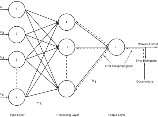
A typical neural network model consists of three layers (input, processing and output layers) and is shown exemplified in Fig.4. The input to a neural network model is a vector of elements xk, where the index k stands for the number of input units in the network (input layer in Fig.4). Input signals are weighted with weights wjkwhere j represents the number of processing units, to give the inputs to the processing units. Weighted input signals are processed if they exceed a certain threshold which is mostly given by a non-linear activation function (e.g., sigmoid functions; in this case the hyperbolic tangent function). Adrian (1926) has shown experimentally that biological neurons respond to a stimulus in a sigmoidal fashion (i.e., no output until a certain threshold is exceeded, followed by a nearly

Table 2 Two regional climate scenarios for the northern part of the Swiss Alps (Frei2004)

P_DJF P_MAM P_JJA P_SON T_DJF T_MAM T_JJA T_SON Scenario 1 No change in climate:1970–2000 mean

Scenario 2 +8% 0% −17% −6% +1.8°C +1.8°C +2.7°C +2.1°C The values refer to the change between the 1970–2000 period and the 2035–2065 period (Frei2004). The time series of winter (DJF), spring (MAM), summer (JJA), autumn (SON) precipitation (P) and temperature (T) are abbreviated as “P_DJF”, “T_DJF”, “P_MAM”, “T_MAM”, “P_JJA”, “T_JJA”, “P_SON” and “T_SON”, respectively

linear input–output relation and saturation from a certain input level onward). After passing the threshold (processing layer in Fig.4), an output signal of the processing layer is yielded. The outputs of the processing units are now fed to the output layer where they are again weighted with the weights Wij. The use of a second activation function will finally produce the output of the network (output layer in Fig.4).

2.4.1 Backpropagation neural networks

There are many types of NN models; some are only of interest to neurological researchers, while others are general nonlinear data techniques applicable in many scientific field. Examples of NN applications in environmental sciences include the analysis of interdecadal changes of El Niño-Southern Oscillation (ENSO) behaviour (Wu and Hsieh2003), efficient radiative transfer computation in atmospheric general circulation models (Chevallier et al. 2000), the detection of anthropogenic climate change (Walter and Schönwiese2002,2003), the production of complete 15-year records of temperature and pressure for six sites across West Antarctic (Reusch and Alley 2004) or the modelling of hydrological processes (Govindaraju2000).

However, in the present study, the standard neural network model, the backpropagation network (BPN), has been applied (Rumelhart et al. 1986). The aim of the learning algorithm (i.e., training a neural network model) is to compare the output signal with the signal to be obtained (target signal, in this study the glacier length). The difference between the real value and the model output result makes the processing unit change the weights set at the previous processing step. As the weights are changed, also a new output signal is produced. The processing unit continues until a sufficient output result is reached, i.e. until

ij

Processing Layer Output Layer

Network Output Observations Error Estimation 1 2 3 k j 2 1 error backpropagation i x x x k x 3 2 1 W Input Layer w jk

Fig. 4 An example of a simplified three-layer k–j–1 BPN architecture. The concept of the backpropagation training algorithm is also shown

a set of coefficients is found that reduces the error between the model outputs and the given test data y(xk). This is usually done by iterative adjustments of the weights wjkand Wijbased on the changing error results to minimize the least square error. One way to adjust these weights is error backpropagation.

The architecture of the backpropagation neural network is based on a supervised learning algorithm to find a minimum cost function. A problem concerning back-propagation neural network is that it does not guarantee that the global minimum of this cost function will be reached, though it is very likely that a minimum good enough to produce responses in the data can be found. Because this approach bears a certain risk of overfitting, the data have to be separated into a training and a validation subset. Using the so called cross-validation technique (Stone1974; Michaelsen1987), the actual“learning” process of the network is performed on the training subset only, whereas the validation subset serves as an independent reference for the simulation quality. When applying neural network models to a non-stationary time series, as in this approach, the training subset includes the full range of extremes in both predictors and predictands. Otherwise, the algorithm will fail during the validation process if confronted with an extreme value that was not part of the training subset. In this study, 75% of all data were used for training and the remaining 25% for validation (Walter and Schönwiese2003).

The backpropagation training consists of two passes of computation: a forward pass and a backward pass. In the forward pass (solid arrows in Fig.4), an input vector is applied to the units in the input layer. The signals from the input layer propagate to the units in the processing layer and each unit produces an output. The outputs of these units are propagated to units in subsequent layers. This process continues until the signals reach the output layer where the actual response of the network to the input vector is obtained. During the forward pass the weights of the network are fixed. During the backward pass (dashed arrows in Fig.4), on the other hand, the weights are all adjusted in accordance with an error signal that is propagated backward through the network against the initial direction. For the present study, seasonal temperature and precipitation data series for the period from 1500 to 2000 (see Section2.2), as well as climate scenarios for the years 2000–2050 (see Section 2.3) were used as input data. This is done because glacier fluctuations are primarily influenced by air temperature, while precipitation is the second most important climatic factor (Kuhn 1981; Oerlemans 2001). Glacier length data from the Lower Grindelwald and Nigardsbreen Glacier served as target function. The backpropagation neural network has therefore to find the connection between the input and target data, which is the core of the“learning” process. In detail, six seasonal climate data were used as forcings (T_MAM, T_JJA, T_SON, P_DJF, P_MAM, P_SON) for the Lower Grindelwald Glacier. Winter temperature (T_DJF) and summer precipitation (P_JJA) have been omitted. For the Nigardsbreen Glacier five forcing time series (T_MAM, T_JJA, T_SON, P_DJF, P_MAM) were used (see Section2.4.3for further comments).

Note that the response of the glacier length to a climate forcing is not immediate but delayed. This is considered by a NNM by the setting of a time lag of 45 years for the Grindelwald input data (see comments below) and a time lag of 20 years for the Nigardsbreen input data (Nesje and Dahl2003). The input data was shifted stepwise so that all lags between 0 and 45 years (Lower Grindelwald Glacier) or 0 and 20 years (Nigardsbreen Glacier) were considered. This was done to account for the reaction time (i.e., the time lag between the reaction of the glacier front to a change in climate parameters) of the glacier. The neural network model chooses those input series which fit best to explain the behaviour of the target function, i.e. the delay of the glacier length to climate stimuli should be recognized correctly.

The used time lag of 45 years for the Lower Grindelwald Glacier is on the one hand based on a simple (optical) analysis of the time lag between a distinct climate signal and the corresponding glacier front reaction of the Lower Grindelwald Glacier. We consider a value of approximately 20–30 years. However, it must be noted that the reaction to climate at the glacier snout can also change in some situations, e.g. after runs of cool summers (Matthews and Briffa2005). Note that Schmeits and Oerlemans (1997) calculated a response time of 34–45 years for the Lower Grindelwald Glacier. This value is the time required for a glacier to adjust from one“steady-state” to another following a change in the mass balance. Usually this time is two to three times longer than the“reaction time” mentioned before (personal communication by Wilfried Haeberli, University of Zurich, 22 January 2007). With a time lag of 45 years as upper bound we therefore ensure that our NN model works with the most significant and influential climatic pre-conditions.

Using too few/many processing units can lead to underfitting/overfitting problems because the simulation results are highly sensitive to the number of processing units and learning parameters. Therefore a variety of backpropagation neural networks must be checked to obtain robust results. As mentioned above, this network architecture still carries the risk of being stuck in local minima on the error hypersurface. To reduce this risk, conjugate gradient descent was used in this study. This is an improved version of standard backpropagation with accelerated convergence. For a detailed description of this technique, see Steiner et al. (2005).

The architecture of the NNM can be chosen, though the model processes well if the number of processing units is set to half the number of input units. This number has been determined after a time-consuming trial and error procedure by repeated simulations with different numbers of processing units and by analyzing the performance on the validation sample (Hsieh 2004; Steiner 2005). Using a time lag from 0 to 45 years for the Lower Grindelwald Glacier, we get 46×6=276 input units (climate variables), 138 processing units in 1 processing layer and the length fluctuations as output unit. This neural network architecture is abbreviated as 276–138–1. In the case of Nigardsbreen Glacier, a 105–53–1 architecture (five forcing time series and a maximal time lag of 20 years) was applied.

An uncertainty in the backpropagation neural network simulation is related to the fact that the identified minimum is dependent on the starting point on the error hypersurface. To reduce this kind of uncertainty, i.e. in order to ensure that the error reduction process does not always follow the exact same path, multiple model runs are needed. The simulations start from different initial conditions, using the training data in different orders. Hence, the backpropagation neural network was performed 30 times, starting from different locations on the error hypersurface. Finally, the average of the 30 model results was analyzed.

2.4.2 Modelling future glacier fluctuations

A first purpose of the neural network model was to use the available length curve of the Lower Grindelwald Glacier for simulating its future glacier length fluctuations (see Section 3.1). For this, the model was fitted with multiproxy reconstructions (input data) covering the time span of the length curve (1535–1983). Before feeding the NN, the data are standardized to the 1535–1983 mean and standard deviation (z-transformation). This is necessary in order to make temperature and precipitation comparable (and independent from elevation) and to allow a robust neural network performance. Note that all climate variables used as input data of the neural network are independent from the glacier length curves which are based on historical documents. The data are then filtered with a 20-year

Gaussian low-pass filter and shifted stepwise so that all lags between 0 and 45 years were considered. The 20-year smoothing is an attempt to move the direct, undelayed input data towards the filtered and delayed glacier length data (target function). After fitting the BPN with the conjugate gradient descent method, the climate variables until 2050 from the two regional climate scenarios (Section 2.3) served as input data to reconstruct a proxy of annual length changes of the Lower Grindelwald Glacier for the 1976–2050 period. In a final step, the data were rescaled by the inverse z-transformation. The sum of 30 model runs was taken as averaging result, confidence intervals are calculated from Root Mean Square (RMS) errors of the predictions. It has to be noted that therefore also the NN model results represent smoothed glacier length data, which has to be taken into account when making statements on shorter time scales (Nussbaumer et al.2007b).

2.4.3 Sensitivity analysis based on neural networks

Neural network models also allow analysing the sensitivity of the Lower Grindelwald and Nigardsbreen Glacier to temperature and precipitation. Sensitivity analysis using neural networks is based on the measurements of the effect that is observed in the output layer due to changes in the input data. After training the BPN one seasonal temperature or precipitation input is kept constant while the other inputs are allowed to fluctuate. The trained model will then be fed with this new pattern. The observed error of glacier response gives indications of its sensitivity to the input that was constant. Thus, the greater the increase in the error function upon restricting the input, the greater the importance of this input in the output (e.g. Wang et al. 2000). This procedure is repeated for each input variable. In order to reduce the effect of falling into local minima, the average of a total of 30 model runs was taken, resulting in varying importance of the input variable (Steiner 2005; Nussbaumer et al.2007a,b).

In this study, a sensitivity analysis of several advance and retreat periods of the Lower Grindelwald (Fig.5) and Nigardsbreen Glacier based on neural networks was performed. Winter (Prec_DJF), spring (Prec_MAM) and autumn precipitation (Prec_SON) as well as spring (Temp_MAM), summer (Temp_JJA) and autumn temperature (Temp_SON) served as input variables for the Lower Grindelwald Glacier. For Nigardsbreen Glacier, winter (Prec_DJF) and spring precipitation (Prec_MAM) as well as spring (Temp_MAM), summer (Temp_JJA) and autumn temperature (Temp_ SON) were used as input variables (see Section 2.2). An analysis of the Seasonal Sensitivity Characteristics (SSCs) of both the Lower Grindelwald and Nigardsbreen Glacier shows that summer (JJA) precipitation and winter (DJF) temperature hardly affect the mass balance and therefore glacier length reaction (Oerlemans and Reichert 2000; Steiner 2005). Furthermore, possible summer snowfall effects cannot be detected by a seasonal mean of summer (JJA) precipitation which does not differentiate between solid and liquid precipitation. Because summer snowfall effects are coupled with low summer (JJA) temperatures, this time series probably contains enough information of potential summer snowfalls. So, the two time series P_JJA and T_DJF are not used as input variables (Oerlemans and Reichert2000; Reichert et al. 2001; personal communication by Johannes Oerlemans, University of Utrecht, 10 August 2005).

As described in Section 2.4.2, the input data for the Lower Grindelwald Glacier was standardized to their mean and standard deviation over the whole training/verification period 1535–1983. Each climate input of the Lower Grindelwald Glacier has been filtered and stepwise shifted in time so that all lags between 0 and 45 years have been used.

In an analogous procedure the input data for Nigardsbreen Glacier has been standardized over the training/verification period 1710–2004 (data from Østrem et al. 1976; with later updates by the Norwegian Water Resources and Energy Directorate (NVE), Section for Glacier and Snow), filtered and shifted stepwise with a maximal time lag of 20 years (Nesje and Dahl2003).

3 Results

3.1 Modelling the response of the Lower Grindelwald Glacier to climate change

A disadvantage of the Lower Grindelwald Glacier is the absence of long-term mass-balance data. Furthermore, most instrumental data series for temperature and precipitation from nearby locations just cover the twentieth century. Therefore, we must rely upon indirect evidence to provide information about climate and glacier variability over the past centuries. Due to the extraordinary low position of the terminus and its easy accessibility the Lower Grindelwald Glacier is one of the world's best-documented glaciers (Holzhauser and Zumbühl 1996; Oerlemans2005). Zumbühl (1980), Zumbühl et al. (1983), Holzhauser and Zumbühl (1999, 2003) used a wealth of historic pictures (drawings, paintings, prints, photographs) to derive a detailed length variation curve of the Lower Grindelwald Glacier back to 1535 (Fig.5).

For the NN model we used precipitation data of Pauling et al. (2006) and temperature data of Luterbacher at al. (2004) and Xoplaki et al. (2005) at grid point 8.25° E/46.75° N (nearest grid point to the Lower Grindelwald Glacier) as independent input data. The above-mentioned glacier length fluctuations of the Lower Grindelwald Glacier (Zumbühl 1980; Zumbühl et al.1983; Holzhauser and Zumbühl2003) served as dependent output dataset of the model. Finally, two regional climate scenarios (Section2.3) were fed to the trained NN

1600 1700 1800 1900 2000 –2000 –1500 –1000 –500 0 Year

Cumulative length changes in meters

1550 1650 1700 1750 1800 1850 1900 1950 2000

advance retreat advance advance retreat advance retreat retreat

Fig. 5 Cumulative length variations of the Lower Grindelwald Glacier from 1535 to 1983, relative to 1855/ 1856 (=0). As a consequence of uncertainties in determining an exact front position from documentary data (drawings, paintings), a spread of possible front positions is given. Maximal extensions of the Lower Grindelwald Glacier are represented by a thick line, maximal extensions (smoothed with a 20-year low-pass filter) by a solid line, and minimal extensions by a dashed line (e.g. Zumbühl1980; Zumbühl et al.1983). Also shown are the advance/retreat periods (grey shaded bands) that are analyzed in Section3.2

model to reconstruct a proxy of annual length changes of the Lower Grindelwald Glacier for the 1976–2050 period.

Figure6shows these reconstructions, i.e. the response of the Lower Grindelwald Glacier to the two regional climate scenarios using the NN procedure described in Section2.4.2. Note for both scenarios the good accordance of observed and simulated glacier variations for the 1976–2004 period which confirms the reliability of the NN predictions.

Figure6a (scenario 1; see Table2) shows a continuous retreat of the glacier until the year 2025 of about−600±200 m (95% confidence interval) compared to 2000. From 2025 onwards the model indicates a glacier advance of about +400±400 m (95% confidence interval). This result is consistent with Oerlemans et al. (1998) who postulated significant growing for the Lower Grindelwald Glacier in the twenty-first century. Note that the projections in Oerlemans et al. (1998) have been made with the assumption that climate conditions will be constant and equal to the average climate conditions over the period 1961–1990. Additionally, in accordance to Steiner et al. (2005) the NN model performs better than a multiple linear regression (MLR) model approach with the same input data as in the NN approach: The MLR model shows a continuous glacier retreat during the first half of the twentieth century and does not simulate the potential glacier advance from 2025 onwards.

Figure6b (scenario 2; see Table2) represents a possible projection of the glacier length due to anthropogenic forcings. After the minor advance in the 1980s the Lower Grindelwald Glacier shows a strong retreat of around −1,400±300 m (95% confidence interval) until the 2050s.

3.2 Precipitation and temperature significance for historic glacier variations– a comparison Glacier length is a function of mass balance and ice dynamics, which in turn are determined by the topography and prevailing climate (including energy balance and albedo). Similar to

1600 1700 1800 1900 2000

–3000

–1000

0

Year

Cumulative length change (meters)

scenario 1

a

Cumulative length change (meters)

scenario 2

b

observed projected

Fig. 6 Filtered cumulative gla-cier length variations of the Lower Grindelwald Glacier for the 1550–2050 period (1550=0). For the 1550–1975 period the thick line represents length fluc-tuations reconstructed from his-torical evidence, for the 1976– 2050 period it is the average of the predictions derived from dif-ferent initial starting points. Also shown is a 95% confidence in-terval (grey shading) around the predictions of cumulative length variations derived from RMS errors of the predictions. The NN was forced with two regional climate scenarios: a scenario 1 (“no change scenario”), b sce-nario 2 (“combined forcing scenario”)

other climate proxies, glacier fluctuations are the product of variations in more than one (meteorological) parameter. It can be delayed and may continue long after the climate has restabilized following a change. Glacier front changes thus need not necessarily to be coupled solely with climate, which complicates climatic interpretations of glacier fluctuations.

In contrast to glacier length, mass balance reacts almost immediately to a change in climatic conditions. It depends mainly on air temperature, solar radiation, and precipitation. Extensive meteorological experiments on glaciers have shown that the primary source for melt energy is solar radiation but that fluctuations in the mass balance through the years are mainly due to temperature during the summer ablation period and precipitation during the winter accumulation period (Oerlemans 2005). Nevertheless, it must be noted that also precipitation in summer as combined with temperature can have very important effects: snowfalls in summer have strong impact on the energy balance during ablation period (Oerlemans and Klok2004). When calculating the mass-balance on present-day glaciers, the accumulation and ablation seasons are regarded to seven (October–April) and five (May–September) months, respectively.

But as glacier mass balance data hardly reach back to the first half of the twentieth century and only exist for few glaciers, glacier length data as a much easier determinable parameter has to be considered as an alternative to study the climate–glacier relation. In an attempt to find consistency between glacier advances and both temperature and precipitation reconstructions we compared the length variations of the Lower Grindelwald Glacier (Switzerland) with precipitation reconstructions by Pauling et al. (2006) and temperature reconstructions by Luterbacher et al. (2004) and Xoplaki et al. (2005).

To investigate the relative importance of influencing climatic factors to the Lower Grindelwald Glacier we performed a sensitivity analysis based on neural networks (see Section 2.4.3) using six climate series (T_MAM, T_JJA, T_SON, P_DJF, P_MAM, P_SON) as input data and the length curve as target function. Figures7and8show the time series used as input data, and Figs. 9 and 10 show boxplots describing the relative importance of the input data for four advance and four retreat periods of the Lower Grindelwald Glacier (Fig. 5; Zumbühl 1980; Zumbühl et al. 1983; Holzhauser and Zumbühl1999,2003). Each boxplot is based on the outputs of 30 model runs with varying initial weights to reduce the effect of falling into local minima (Steiner et al. 2005; Nussbaumer et al.2007b). For each input variable the median, the first and third quartile (lower/upper hinge) and the lower/upper whiskers of the 30 model runs are given. Note that the whiskers are extended to the farthest points within 1.5 interquartile ranges from the first to the third quartile. Besides varying importance of the input variables, i.e. changing climatic configurations that led to the four main advances of the Lower Grindelwald Glacier in the 1550–1850 period (see Table3 for the main climatic combinations that led to the glacier advances and retreats), we also found changing variability of input importance. High variability, for example, could indicate a lower ability of the NN model to generalize the pattern beyond the used input/output data.

The 1590–1610 advance (Fig.9a) seems to be driven by low summer and low spring temperatures. Autumn precipitation plays a secondary role. It is surprising that the above-average winter precipitation before and during this advance period is not shown as significant. The 1690–1720 advance was likely triggered by low spring temperature and high spring precipitation (Fig.9b). High precipitation and low summer temperatures could have been the driving factors of the short, but well pronounced 1760–1780 glacier advance (Wanner et al. 2000). The 1810–1820 advance, which marks the beginning of the mid-nineteenth century maximum glacier extent, was presumably driven by low summer

temperatures and high autumn precipitation (Fig. 9d). In this case the variability of the relative importance is lower compared to the other advance periods. Furthermore, this advance shows specifically the expected pattern of an advancing Alpine glacier: Above normal (autumn) precipitation leads to a positive mass balance in the accumulation area,

1500 1600 1700 1800 1900 2000 –3 –2 –1 0 12 3 Year

Standardized winter (DJF) precipitation

a 1500 1600 1700 1800 1900 2000 – 3 – 2 – 1 0123 Year

Standardized spring (MAM) precipitation

b 1500 1600 1700 1800 1900 2000 – 3 – 2 – 1 0123 Year

Standardized autumn (SON) precipitation

c

Fig. 7 Standardized precipitation values for the 1500–2000 period (solid lines) at the grid point 8.25° E/ 46.75° N (Lower Grindelwald Glacier; after Pauling et al.2006): a winter (DJF) precipitation, b spring (MAM) precipitation, c autumn (SON) precipitation. Also shown are the 20-year low-pass filtered time series of the precipitation model inputs (thick lines). The time series are z-standardized relative to the 1535–1983 mean and standard deviation

which is a prerequisite for later advances of the glacier snout. Low summer temperatures during the advance period hinder ablation making glacier advances possible.

It is not surprising that the four retreat periods were mainly driven by high temperatures (Fig.10a–d). The 1640–1665 retreat seems to be triggered by high summer temperatures and low spring and autumn precipitation (Fig.10a). A typical pattern of retreating glaciers

1500 1600 1700 1800 1900 2000 –3 –2 –1 0 1 23 Year

Standardized spring (MAM) temperature

a

Standardized summer (JJA) temperature

b

Standardized autumn (SON) temperature

c

Fig. 8 Standardized temperature values for the 1500–2000 period (solid lines) at the grid point 8.25° E/46.75° N (Lower Grindelwald Glacier; after Luterbacher et al.2004; Xoplaki et al.2005): a spring (MAM) temperature, b summer (JJA) temperature, c autumn (SON) temperature. Also shown are the 20-year low-pass filtered time series of the temperature model inputs (thick lines). The time series are z-standardized relative to the 1535–1983 mean and standard deviation

Prec_DJFPrec_MAM Prec_SON Temp_MAM Temp_JJA Temp_SON 0 2 04 06 08 0 1590–1610 advance Model input

Relative input importance in %

a

Prec_DJFPrec_MAM Prec_SON Temp_MAM Temp_JJA Temp_SON

02 0 4 0 6 0 8 0 1690–1720 advance Model input

Relative input importance in %

b

Prec_DJFPrec_MAM Prec_SON Temp_MAM Temp_JJA Temp_SON

0 2 04 06 08 0 1760–1780 advance Model input

Relative input importance in %

c

Prec_DJFPrec_MAM Prec_SON Temp_MAM Temp_JJA Temp_SON

0 2 04 06 08 0 1810–1820 advance Model input

Relative input importance in %

d

Fig. 9 Relative importance of climate input variables to length fluctuations of the Lower Grindelwald Glacier (Switzerland) for four advance periods: a 1590–1610, b 1690–1720, c 1760–1780 and d 1810–1820. For each input variable the median, the first and third quartile (lower/upper hinge) and the lower/upper whisker of the 30 model runs are given

Prec_DJFPrec_MAM Prec_SON Temp_MAM Temp_JJA Temp_SON

0 2 04 06 08 0 1640–1665 retreat Model input

Relative input importance in %

a

Prec_DJFPrec_MAM Prec_SON Temp_MAM Temp_JJA Temp_SON

0 2 04 06 0 8 0 1780–1810 retreat Model input

Relative input importance in %

b

Prec_DJFPrec_MAM Prec_SON Temp_MAM Temp_JJA Temp_SON

02 0 4 0 6 0 8 0 1860–1880 retreat Model input

Relative input importance in %

c

Prec_DJFPrec_MAM Prec_SON Temp_MAM Temp_JJA Temp_SON

02 0 4 0 6 0 8 0 1945–1970 retreat Model input

Relative input importance in %

d

Fig. 10 Relative importance of climate input variables to length fluctuations of the Lower Grindelwald Glacier (Switzerland) for four retreat periods: a 1640–1665, b 1780–1810, c 1860–1880 and d 1945–1970. For each input variable to the neural network the median, the first and third quartile (lower/upper hinge) and the lower/upper whisker of the 30 model runs are given

can be seen in the 1780–1810 period (Fig.10b): High overall temperatures and low winter precipitation enhance ablation while accumulation during winter season is reduced. High spring temperatures and decreasing autumn precipitation could have been the cause for the 1860–1880 retreat (Fig.10c). Finally, the 1945–1970 retreat could have been driven by high spring and autumn temperature and low autumn precipitation (Fig.10d). It has to be noted that in this case the variability of the relative importance is higher compared to the other retreat periods.

We performed the same sensitivity study for Nigardsbreen, W-Norway (7°08′ E, 61°45′ N). In an analogous procedure as described above the relative importance of five input series (T_MAM, T_JJA, T_SON, P_DJF, P_MAM) for one advance and retreat period have been evaluated (Fig.11).

Table 3 Major advance/retreat periods of the Lower Grindelwald Glacier and the combinations of seasonal temperature and precipitation (forcings) which led to the described glacier variations

Period Climate variables

Advance 1590–1610 P_SON, T_MAM, T_JJA

Advance 1690–1720 P_MAM, T_MAM

Advance 1760–1780 P_DJF, P_MAM, P_SON, T_JJA

Advance 1810–1820 P_SON, T_JJA

Retreat 1640–1665 P_MAM, P_SON, T_JJA

Retreat 1780–1810 P_DJF, T_MAM, T_JJA, T_SON

Retreat 1860–1880 P_SON, T_MAM

Retreat 1945–1970 P_SON, T_MAM, T_SON

In bold, most important forcing data series

Prec_DJF Prec_MAM Temp_MAM Temp_JJA Temp_SON

02 0 4 0 6 0 8 0 1710–1748 advance Model input

Relative input importance in %

a

Prec_DJF Prec_MAM Temp_MAM Temp_JJA Temp_SON

02 0 4 0 6 0 8 0 1945–1970 retreat Model input

Relative input importance in %

b

Fig. 11 Relative importance of climate input variables to length fluctuations of the Nigardsbreen for: a the advance period 1710–1748 and b the retreat period 1945–1970. For each input variable the median, the first and third quartile (lower/upper hinge) and the lower/upper whisker of the 30 model runs are given

Interestingly, very high spring precipitation was reconstructed from 1700 to around 1740 (Fig. 12). This period of extremely high spring precipitation coincides precisely with advances of Nigardsbreen, described by Nesje and Dahl (2003). They report advances of 2,800 m in the 1710–1735 period and another advance of 150 m between 1735 and the historically documented “Little Ice Age” maximum in 1748 (Nesje and Dahl 2003). Additionally, Nigardsbreen Glacier retreated only slightly until at least 1790. Given a frontal lag time to net mass-balance perturbations of 20 years (Nesje and Dahl2003) this matches rather well our high spring precipitation amounts between 1700 and 1740. Additionally, summer temperature proved to be lower than normal during this period, which may also have promoted glacier advances (Fig.13).

The 1710–1748 advance (and the following large extent 1748–1790) seem to be forced by high spring and increasing winter precipitation, low summer and decreasing autumn temperatures (Fig. 11a). Although we use only two precipitation input variables for sensitivity analysis we found a significant contribution to positive glacier length variations. The 1945–1970 retreat is mainly driven by low spring precipitation and high autumn temperatures (Fig.11b).

4 Discussion

4.1 Simulation of future glacier length variations

The simulation of future glacier length variations of the Lower Grindelwald Glacier for scenario 1 and scenario 2 shows a retreating glacier at the beginning of the twenty-first century (Fig.6). For scenario 1 (“no change”) the glacier retreat is weaker and is expected to end in 2025. Afterwards, a significant growing period can be seen. This advance could be explained by a memory effect of the glacier: During the 1970–2000 period winter, spring and autumn precipitation were above average so that mass accumulation could have taken place. Furthermore, in the 2020s the glacier could reach a new equilibrium from which glacier advances are more likely.

As a result of climate scenario 2 (“combined forcing”) the Lower Grindelwald Glacier shows a strong continuous retreat. By comparing this model output with climate scenarios in which only temperature or precipitation forcings are used, we can show that the Lower Grindelwald Glacier is mainly driven by temperature. High precipitation can weaken the retreat of the glacier, but the model outputs do not differ significantly from the outputs of scenarios 1 or 2.

These results are in good agreement with earlier studies which showed predominant influence of temperature in case of fast atmospheric warming (e.g. Kuhn 1981). It has indeed been used for scenario calculations – even for the entire Alps (Oerlemans et al. 1998; Zemp et al.2006).

It must be noted that the simulations mentioned before have been done under twentieth century glacier conditions. Today, further retreat of the glacier is heavily influenced by non-climatic factors such as lake formation, downwasting and disintegration into several sub-glaciers and ice avalanching on steep slopes.

4.2 Climate parameters and historic glacier variations

The relative importance of climate data to glacier advances shows changing patterns during the last 500 years, i.e. during the“Little Ice Age”. There were periods with spring/summer

temperatures being the main driving factors of glacier advances. Thus, low temperatures cause a low ablation rate in the spring/summer/autumn months. Nevertheless, in most cases high precipitation during the accumulation season contributes as well to positive mass balance and glacier advances. High winter precipitation rates together with average/low summer temper-atures normally cause positive mass balance, a decisive prerequisite for glacier advances.

1500 1600 1700 1800 1900 2000 –3 –2 –1 0 1 2 3 Year Standardized winter (DJF) precipitation

_a

1500 1600 1700 1800 1900 2000 – 3 – 2 – 1 0123 Year Standardized spring (MAM) precipitation

_b

Fig. 12 Standardized precipitation values for the 1500–2000 period (solid lines) over the Nigardsbreen region 5–7° E/60–62° N (DJF) and a highly correlated region in N-Sweden 17–20° E/63–65° N (MAM; after Pauling et al.2006): a winter (DJF) precipitation, b spring (MAM) precipitation. Also shown are the 20-year low-pass filtered time series of the precipitation model inputs (thick lines). The time series are z-standardized relative to the 1535–1983 mean and standard deviation

The clearest results are the sensitivity analysis of the 1810–1820 advance and the 1860– 1880 retreat of the Lower Grindelwald Glacier (Figs.9d and 10c). During the 1810–1820 advance summer temperature seems to be the most important factor and autumn precipitation the second factor of importance. For the 1860–1880 retreat spring temperature and autumn precipitation show a significant influence. The other inputs proved to be negligible.

1500 1600 1700 1800 1900 2000 –3 –2 – 1 012 3 Year

Standardized spring (MAM) temperature

a 1500 1600 1700 1800 1900 2000 –3 –2 – 1 0123 Year

Standardized summer (JJA) temperature

b 1500 1600 1700 1800 1900 2000 –3 –2 –1 0123 Year

Standardized autumn (SON) temperature

c

Fig. 13 Standardized temperature values for the 1500–2000 period (solid lines) over the Nigardsbreen region 5–7° E/60–62° N (after Luterbacher et al. 2004 and Xoplaki et al. 2005): a spring (MAM) temperature, b summer (JJA) temperature, c autumn (SON) temperature. Also shown are the 20-year low-pass filtered time series of the temperature model inputs (thick lines). The time series are z-standardized relative to the 1535–1983 mean and standard deviation

The 1590–1610 advance gives similar results though spring temperature becomes equally relevant. The importance of precipitation for the 1760–1780 advance is remarkable. The observed differences between the input importance for these two advance events can be attributed to different reasons. First, it is conceivable that different climate configurations may lead to positive mass balances and thus advances of the glacier. However, the uncertainties of the influences are considerable in many cases. This advance was quite short but well marked. One may argue that also glacier dynamics has played a role. Abundant meltwater in combination with high inclination of the lower parts of the glacier may accelerate glacier speed leading to advances that are not exclusively due to climatic conditions. In 1760 the Lower Grindelwald Glacier ended above steep rocks (Zumbühl et al.1983). The subsequent advance may have been amplified by this topographical feature. However, also other Alpine glaciers like the Rhône and the Rosenlaui Glaciers (Swiss Alps) advanced considerably during that period (Zumbühl and Holzhauser1988). Another reason may be the decreasing quality of the reconstructions further back in time (Luterbacher at al. 2004; Xoplaki et al.2005; Pauling et al.2006). However, during the late eighteenth century both temperature and precipitation have been skillfully reconstructed and the pattern of importance is similar in three of four advance periods (Fig. 9). Hence, we argue that precipitation was the main reason for the 1760–1780 advance.

A striking feature is the importance of autumn precipitation, especially for the 1810– 1820 advance. Precipitation in autumn may already fall as snow on large parts of the glacier which increases the albedo. This equals to a shortening of the ablation period that promotes positive mass balance.

The 1640–1665 retreat was triggered by decreasing spring and autumn precipitation and increasing summer temperature. This is a typical feature of a retreating glacier: High temperatures lead to strong ablation. Due to the low precipitation amounts insufficient mass accumulation takes place resulting in negative mass balance.

A similar pattern can be seen during the 1780–1810 and 1945–1970 retreat periods. High temperatures and in second order low precipitation have been producing negative mass balance and thus glacier retreat. It must be noted that the 1780–1810 retreat is situated within the last part of the Little Ice Age, a well-known glacier-friendly period. Vincent et al. (2005) studied the glacier variations at the end of the Little Ice Age (1760–1830) and argue that the advance of glaciers in the Alps during the mentioned period conflicts with the high summer temperature signal. Because Vincent et al. (2005) analyzed the 1760–1830 period as a whole, our results disagree with the previous statement. On the one hand, we found even a glacier retreat within this period (1780–1810), on the other hand summer temperature contributes significantly to this retreat.

Regarding the early eighteenth century advance of Nigardsbreen, the most striking feature is the high importance of winter and spring precipitation relative to the other input factors used. This is in good agreement with Nesje et al. (2008) who show that an annual glacial advance rate in the order of∼100±20 m during the late seventeenth/early eighteenth century is best explained by increased winter precipitation and thus high snowfall on the glaciers due to prevailing mild and humid winters. However, summer temperatures alone were not sufficiently low.

Note that also spring precipitation is high during the whole advance period whereas winter precipitation is increasing during this period. It is well known that western Scandinavian glaciers are sensitive to changes in winter precipitation (winter included the entire accumulation season October–April; Nesje et al.2000; Nesje and Dahl2003), which is largely determined by the state of the North Atlantic Oscillation (NAO) but the importance of spring precipitation is still striking. Regarding the inferred low summer

temperatures during that period, the real accumulation season may have been longer than at present. Thus, the accumulation during the entire spring period could have contributed to the observed glacier advance even though winter precipitation is not specifically high. However, the early eighteenth century is by far the wettest period in that region over the whole reconstruction period.

The 1945–1970 retreat of Nigardsbreen is mainly triggered by low spring precipitation. This time series shows a very similar run of the curve as the length variations of Nigardsbreen, with a lag of about 10 years. The high autumn temperatures imply an extended ablation period.

From a methodological point of view it can be argued that precipitation is possibly underestimated by the sensitivity analysis presented here. As the training data set includes only limited information on past climatic conditions (maximum time lag=45 or 20 years), it can be supposed that the model does not take into account mass that accumulated more than 45/20 years before the beginning of an advance. On the other hand, the melting effect of high summer temperature is immediately visible.

The influence of precipitation on length variations of the Lower Grindelwald Glacier is smaller than in the case of Nigardsbreen. This can be due to the more southerly location of the Alps in the transition zone between maritime and continental regimes, which makes (summer) temperature the dominating factor, whereas Nigardsbreen is more sensitive to precipitation during the accumulation season. Notice that surprisingly the SSCs of the Lower Grindelwald Glacier and Nigardsbreen Glacier (Oerlemans and Reichert2000) are rather similar: Both glaciers show a low sensitivity in summer (JJA) precipitation and winter (DJF) temperature. Besides the expected high sensitivity in summer (JJA) temperature and winter (DJF) precipitation, a rather high sensitivity in “spring” (AM) temperature (Lower Grindelwald Glacier), resp.“autumn” (SO) temperature (Nigardsbreen Glacier) can be seen. However, these results have shown that also high precipitation is needed before the advances to ensure positive mass balance in the accumulation region of the glacier. This precipitation can fall during different seasons. It could be shown that also autumn (from September onwards) may well contribute to glacier advances.

5 Conclusions and outlook

Using spatially and temporally highly resolved temperature and precipitation reconstruc-tions we could simulate future glacier length variareconstruc-tions of the Lower Grindelwald Glacier, Switzerland, forced by two different climate scenarios. Scenario 1 (“no change scenario”) shows a retreat of the glacier until the year 2025 with a little advance from 2025 onwards. Scenario 2 (“combined forcing scenario”) shows a strong retreat of the glacier until the 2050s. It must be assumed that scenario 2 likely lies ahead of us (climate change).

It has also been demonstrated that the relative importance of seasonal variations of temperature and precipitation has been variable in historic times and that various combinations of temperature/precipitation characteristics can lead to advances/retreats of a glacier in historic times. In particular, precipitation plays an important role in the behaviour of the Nigardsbreen Glacier in western Norway. The Lower Grindelwald Glacier proved to be less sensitive to precipitation and more sensitive to temperature than Nigardsbreen Glacier.

This analysis has been done using NN approaches which differ from classical models (and also from linear statistical methods) in that it uses a nonlinear approach. As the climate system (including the glacier system) can be seen as nonlinear, it has to be questioned

whether traditional linear statistical models are able to describe the full complexity of the system's behaviour. The nonlinear NNMs therefore combine the advantages of physically motivated (possibly nonlinear) climate models, with high complexity, and linear statistical models (e.g. multiple linear regression methods), with a low CPU time demand. A disadvantage of NNs is that the results are strongly dependent on the choice of initial parameter values and initial design decisions. Solid experience is therefore needed for handling with these problems. However, NNMs can be seen as new complementary statistical approaches for analyzing the complex climate–glacier relation and simulating glacier variations in an easy and useful way. Because the limitations and chances of these techniques are not yet fully explored, further investigations towards a“neuro-glaciology”, including the study of changing lags over time or the significance of climate modes (e.g. North Atlantic Oscillation), should be done for different glaciers and in different climate regions.

Acknowledgements This study was supported by the Swiss National Science Foundation (SNSF) through its National Centre of Competence in Research on Climate (NCCR Climate), project PALVAREX.

This work is also part of the EU-Project SOAP (Simulations, Observations and Palaeoclimate Data: Climate Variability over the Last 500 Years), the Swiss contribution being funded by the Staatssekretariat für Bildung und Forschung (SBF), under contract 01.0560.

The authors also wish to thank the following institutions for access to their data: The Federal Office of Meteorology and Climatology (MeteoSwiss), Zürich; the Norwegian Meteorological Institute (met.no), Oslo; the Climatic Research Unit (CRU), Norwich, and the Tyndall Centre for Climate Change Research, Norwich, UK.

Thanks also go to Johannes Oerlemans, Utrecht University, the Netherlands, for the calculation of the Seasonal Sensitivity Characteristic (SSC) of the Lower Grindelwald Glacier.

The detailed comments and suggestions of the Scientific Editor, Stephen H. Schneider, Wilfried Haeberli and an anonymous reviewer helped to improve this paper.

References

Adrian E (1926) The impulses produced by sensory nerve endings. Part I. J Physiol (Lond) 61:49–72 Brázdil R, Pfister C, Wanner H, von Storch H, Luterbacher J (2005) Historical climatology in Europe– the

state of the art. Clim Change 70:363–430

Chevallier F, Morcrette JJ, Cheruy F, Scott NA (2000) Use of a neural-network-based long-wave radiative-transfer scheme in the ECMWF atmospheric model. Q J R Meteorol Soc 126(563):761–776

Chinn T, Winkler S, Salinger MJ, Haakensen N (2005) Recent glacier advances in Norway and New Zealand: a comparison of their glaciological and meteorological causes. Geogr Ann 87A(1):141–157 Frei C (2004) Die Klimazukunft der Schweiz – Eine probabilistische Projektion. Working paper for the

OcCC project“Switzerland in 2050”, OcCC, Bern, 8 pp

Govindaraju RS (2000) Artificial neural networks in hydrology. II: hydrologic applications. J Hydrol Eng 5 (2):124–137 DOI10.1061/(ASCE)1084-0699(2000)5:2(124)

Haeberli W (2006) Integrated perception of glacier changes: a challenge of historical dimensions. In: Knight PG (ed) Glacier science and environmental change. Blackwell, Oxford, pp 423–430

Haeberli W, Hoelzle M (1995) Application of inventory data for estimating characteristics of and regional climatic-change effects on mountain glaciers: a pilot study with the European Alps. Ann Glaciol 21:206–212 Hoelzle M, Haeberli W, Dischl M, Peschke W (2003) Secular glacier mass balances derived from cumulative

glacier length changes. Glob Planet Change 36:295–306

Holzhauser H, Zumbühl HJ (1996) To the history of the Lower Grindelwald Glacier during the last 2800 years– palaeosols, fossil wood and historical pictorial records–new results. Z Geomorphol, Suppl Bd 104:95–127

Holzhauser H, Zumbühl HJ (1999) Glacier Fluctuations in the Western Swiss and French Alps in the 16th Century. Clim Change 43(1):223–237 DOI10.1023/A:1005546300948