On the problem of optimal approximation of the four-wave kinetic integral
Texte intégral
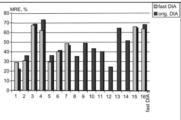
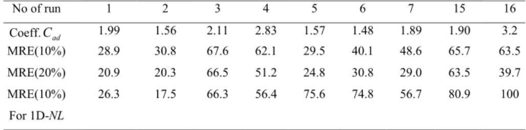
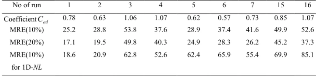
Figure

Documents relatifs
In section 4, we point out the sensibility of the controllability problem with respect to the numerical approximation, and then present an efficient and robust semi-discrete scheme
Precisely, for small values of the damping potential a we obtain that the original problem (P ) is well-posed in the sense that there is a minimizer in the class of
notion of initial data average observability, more relevant for practical issues, and investigate the problem of maximizing this constant with respect to the shape of the sensors,
We gave a scheme for the discretization of the compressible Stokes problem with a general EOS and we proved the existence of a solution of the scheme along with the convergence of
A standard Galerkin mixed method (G) and the Galerkin method enriched with residual-free bubbles (RFB) for equal order linear elements are considered to approximate the displacement
Modélisation mathématique et Analyse numérique Mathematical Modelling and Numerical Analysis.. APPROXIMATION OF A QUASILINEAR MIXED PROBLEM 213 which is not a priori well defined.
M 2 AN Modélisation mathématique et Analyse numérique 0399-0516/87/03/445/20/$4.00 Mathematical Modelling and Numerical Analysis © AFCET Gauthier-Villa r s.. A variational
For the approximation of solutions for radiation problems using intégral équations we refer to [3], [9], [16], [17] in the case of smooth boundaries and to [21] in the case of
