HAL Id: hal-00317224
https://hal.archives-ouvertes.fr/hal-00317224
Submitted on 1 Jan 2004
HAL is a multi-disciplinary open access
archive for the deposit and dissemination of
sci-entific research documents, whether they are
pub-lished or not. The documents may come from
teaching and research institutions in France or
abroad, or from public or private research centers.
L’archive ouverte pluridisciplinaire HAL, est
destinée au dépôt et à la diffusion de documents
scientifiques de niveau recherche, publiés ou non,
émanant des établissements d’enseignement et de
recherche français ou étrangers, des laboratoires
publics ou privés.
ofradars within the PSMOS-DATAR Project
A. H. Manson, C. E. Meek, C.M. Hall, S. Nozawa, N.J. Mitchell, D. Pancheva,
W. Singer, P. Hoffmann
To cite this version:
A. H. Manson, C. E. Meek, C.M. Hall, S. Nozawa, N.J. Mitchell, et al.. Mesopause dynamics from the
scandinavian triangle ofradars within the PSMOS-DATAR Project. Annales Geophysicae, European
Geosciences Union, 2004, 22 (2), pp.367-386. �hal-00317224�
Annales Geophysicae (2004) 22: 367–386 © European Geosciences Union 2004
Annales
Geophysicae
Mesopause dynamics from the scandinavian triangle of radars
within the PSMOS-DATAR Project
A. H. Manson1, C. E. Meek1, C.M. Hall2, S. Nozawa3, N.J. Mitchell4, D. Pancheva5, W. Singer6, and P. Hoffmann6
1Institute of Space and Atmospheric Studies, University of Saskatchewan, Canada
2Tromsø Geophysical Observatory, University of Tromsø, Norway
3Solar-Terrestrial Environment Laboratory, University of Nagoya, Japan 4Department of Electronic and Electrical Engineering, University of Bath, UK
5Department of Physics, University of Wales, UK
6Leibniz-Institute of Atmospheric Physics, K¨uhlungsborn, Germany
Received: 4 February 2003 – Revised: 2 July 2003 – Accepted: 22 July 2003 – Published: 1 January 2004
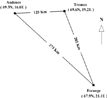
Abstract. The “Scandinavian Triangle” is a unique trio of
radars within the DATAR Project (Dynamics and Tempera-tures from the Arctic MLT (60–97 km) region): Andenes MF radar (69◦N, 16◦E); Tromsø MF radar (70◦N, 19◦E) and Esrange “Meteor” radar (68◦N, 21◦E). The radar-spacings range from 125–270 km, making it unique for studies of wind variability associated with small-scale waves, comparisons of large-scale waves measured over small spacings, and for comparisons of winds from different radar systems. As such it complements results from arrays having spacings of 25 km and 500 km that have been located near Saskatoon. Correla-tion analysis is used to demonstrate a speed bias (MF smaller than the Meteor) between the radar types, which varies with season and altitude. Annual climatologies for the year 2000 of mean winds, solar tides, planetary and gravity waves are presented, and show indications of significant spatial vari-ability across the Triangle and of differences in wave charac-teristics from middle latitudes.
Key words. Meteorology and atmospheric dynamics
(mid-dle atmosphere dynamics; waves and tides: instrument and techniques)
1 Introduction
The spatial and temporal variability of the wind and wave fields of the Mesosphere and Lower Thermosphere (MLT; 60–110 km) remain one of the least well-studied and
understood aspects of atmospheric dynamics. The MFR
(Medium Frequency Radars) of the Canadian prairies have contributed significantly to our existing knowledge.
We provide a brief review of the relevant studies. The first involved GRAVNET, an MFR network designed to
charac-Correspondence to: A. H. Manson
terize Gravity Waves (GW) (Manson and Meek, 1988). It featured not one, but three spaced-antenna receiving arrays in a triangle of side about 40 km. The winds obtained from each array were very similar, but their temporal variability and cross-spectral analysis provided unique GW characteristics (periods, 10- 300 min; horizontal wavelengths, 40–1200 km). This system was followed by the addition of two complete MFR systems to the main system at Saskatoon, forming a triangle of side near 500 km. It became clear that the clima-tologies, for example, monthly profiles, of mean winds and tides were very similar and consistent; but that fluctuations in the daily values of all wave-types (tides, planetary and grav-ity waves), with time scales of 4 to 365 days, were highly correlated across the triangle at given altitudes (60–88km) (Hall et al., 1995a). An unexpected result was that for the two GW bands (10–100 min, 2–6 h) correlations between sites (500 km spacings) at a given height were higher than between neighbouring layers (15 km separation) at any site. Although some horizontal uniformity was expected, such al-titude variability in GW propagation conditions was interest-ing and informative (for example, Zhong et al., 1996). Cou-pling between wave-types was noted. A companion paper (Hall et al., 1995b) focussed on inertial GW (2–10 hour pe-riod) and was consistent with the first study in that tempo-ral hodographs at specific heights were much more regular or coherent than were oscillations over a 20 km height inter-val at a particular time. It was also frequently the case that although an oscillation due to an inertial GW could be iden-tified at each (500 km) site, the frequency characteristics of those oscillations were often different, indicating dispersion of the wave and wave-packet over 500 km. This made cross-spectral analysis methods of determining the GW character-istics challenging or impossible. Nevertheless, useful GW characteristics and climatologies were determined.
The development of observing systems in Northern Scan-dinavia and the Arctic has serendipitously provided a triangle
Fig. 1. Map of the three MLT radar locations.
of MLT radars, which is ∼50% of the size of the 500 km Canadian Prairies’ array: the Scandinavian-Triangle or S-Triangle. There is a “Meteor Wind Radar” (MWR) at Es-range, and MFRs at Tromsø (co-located with EISCAT) and Andenes (co-located with ALOMAR), which are described in Sect. 2. The dimensions and positions for this “Scandina-vian Triangle” are shown in Fig. 1. Topics of interest to the community have changed since the studies discussed above, so we shall not simply repeat those, although some themes will re-appear here. A topic of great interest, encouraged by SCOSTEP’s PSMOS (Planetary Scale Mesopause Observing System, 1998–2002) Programme, is the spatial variability of local oscillations in the wind-field, i.e. 12-, 24-h ties that are manifestations of the tide, and 2-, 16-d periodici-ties that are manifestations of Planetary Waves (PW). Both of these wave-types are global phenomena, since they are theo-retically described by Hough modes, but smaller scale struc-tures co-exist with them. Examples include non-(solar) mi-grating tidal modes, which are clearly seen in recent analysis of HRDI (High Resolution Doppler Interferometer) satellite data (Manson et al., 2002a).
We have also recently completed studies of winds and wave-types (tides, planetary waves (PW), and GW) for a network of middle-latitude MFRs called CUJO: Canada
U.S. Japan Opportunity. The locations are London (43◦N,
81◦W), Platteville (40◦N, 105◦W), Saskatoon (52◦N,
107◦W), Wakkanai (45◦N, 141◦E), Yamagawa (31◦N,
131◦E), and offer separations of 1000–7000 km in
longi-tude and 12 degrees (circa 1200 km) in latilongi-tude. As with the HRDI-tidal study mentioned above, longitudinal variations in tidal characteristics (and PW) were very significant, often being larger than over 12 degrees of latitude (at a common longitude). The analysis used in these two papers (Manson et al., 2003a, 2004a will be repeated here, as will references to similarities in spatial effects.
Here we compare winds across the triangle in a correla-tion technique that provides a unique height calibracorrela-tion and speed-ratio assessments between radar types (Sect. 4). An-nual climatologies of mean winds, tides, and PW are shown in Sections 3, 5, and 6. Also, in Sect. 7, the temporal variabil-ities of GW variances (2–6 h periods) are compared across the Triangle. The opportunity to compare wind observations from different MLT radar types is valuable and receives ap-propriate discussion (Sections 4 and 8).
2 Radars and Data Analysis
2.1 Radars
The Tromsø MF radar (2.78 MHz) is located at the EISCAT site of Ramfjordmoen (70◦N, 19◦E) and has been described in the recent papers already referenced, and in particular by Hall (2001). The spaced antenna “full correlation analysis” (FCA) method is used (Meek, 1980). Vertical soundings pro-vide wind sampling at 3-km intervals every 5 min from near 60 to 120 km. The Andenes MFR (1.98 MHz), which is lo-cated at the ALOMAR site (69◦N, 16◦E), is effectively of the same design (including electronics and antenna system), although the winds are available at 2 km and 2 min intervals. It uses the more classical method of analysis due to Briggs (1984). Comparisons have shown that no significant differ-ences exist between these methods (Thayaparan et al., 1995). It is important to note that despite design similarities in the antennas there could be operational differences between the Tromsø and Andenes systems: factors include the ground-plane, and coupling with neighbouring antenna systems (this latter could be more significant for the Tromsø MFR). For the analyses described in Sect. 2.2 the basic data product is usually the hourly mean, but to be consistent with the meteor radar a 2-h mean formed every hour is also used.
The new University of Bath meteor radar (MWR) is lo-cated at Esrange (68◦N, 21◦E), which is the Swedish Space Corporation’s rocket range near Kiruna in Northern Sweden. The radar uses a transmitter of 6 kW peak power, and op-erates at a frequency of 32.5 MHz. Crossed-element Yagi antennas are used for both transmitting and receiving. A sin-gle antenna acts as the transmitter and five separate antennas are used as receivers. The radar operates in an “all-sky” con-figuration, with radiated power being largely independent of azimuth. The five individual receiver antennas form an inter-ferometer to determine meteor echo azimuth and elevation angles. The elevation angle measurements, in combination with measurements of the echo range, allow for meteor-echo heights to be estimated, with a height resolution of typically
<2 km. The MLT circle from which meteors are detected is of diameter 500 km, with a median (horizontal) range of circa 130km; there is a rather uniform azimuthal distribution of detected meteors; and the diurnal variation of detected mete-ors, while peaking near 05:00 UT, is modest and not thought to affect the analysis of tides during the year (Mitchell et al., 2002). (In comparison, the MLT circle from which MFR
A. H. Manson et al.: Mesopause dynamics:The PSMOS-DATAR project 369 echoes are acquired is of diameter near 60km (Meek et al.,
1986).) Continuous data collection commenced on 5 Au-gust 1999. A detailed description of the various steps in the data processing techniques used to discriminate between echoes from meteors and all other signals is give by Hock-ing et al. (2001). In this paper the data have been assigned to the nearest 3 km height interval, as used by the MFR at Tromsø, for convenience in forming contour plots through-out the MLT region (see Sect. 2.2 below). The basic data products are 2-h means that are formed every hour.
Since all wind measurement systems potentially have bi-ases or selectivity issues, some comment about the accu-racy of the radar-winds is appropriate. Examples of sys-tem comparisons include an MFR and Meteor Wind Radar
(MWR) at 43◦N (Hocking and Thayaparan, 1997); MFRs
and Fabry-Perot Interferometers (“green line” and hydroxyl)
at two 52◦N locations (Manson et al., 1996; Meek et al.,
1997); and rockets and radars (MFR, VHF and EISCAT) near 70◦N (Manson et al., 1992). In all of these studies the phases of the tides, or directions of the winds, have gener-ally been satisfactorily consistent, for example, means within
standard errors, as assessed by the authors. The
Saska-toon optical-MFR comparisons showed no speed biases, but “SKiYMET” MWR-MFR speed-comparisons at Saskatoon during the summer of 1998 have shown modest differences, for example, MWR/MFR ratios of about 1.33 (Meek, Hock-ing and Manson, Private Communication, 2002) at 88 km al-titude; and for similar altitudes at 70◦N, Tromsø, the speeds
from the MFR were smaller by a factor of 1.54 than those from other systems. For our purposes here, we will bear in mind the potential biases between different experiments when any later comparisons are made in this paper. There will also be an opportunity to specifically compare the MWR and MFR speeds across the Triangle.
2.2 Analysis techniques
To provide an annual climatology of atmospheric oscillations from 5-h to 30-d at a chosen height a wavelet analysis is ap-plied to a year of hourly mean winds with additional data at the ends, if available, to cover the full sliding window for all wave periods used (Fig. 2). A Gaussian window of length 6 times the period (truncated at 0.05 of peak value) is used to approximate a Morlet wavelet analysis (Kumar and Foufoula-Georgiou, 1997), but one in which gaps do not have to be filled. Criteria for the existence of data are described later. A Fourier transform (not an FFT) is therefore used and applied to existing data points only. Each time-axis pixel (800 are used) represents several hours, since the axis covers 1 year. Breaks in the heavy data-existence line at the bot-tom of the frame indicates that there were no data for those hours, and are a warning that spectral data near the edges of, and during, these intervals may be inaccurate. The period-scale uses 600 pixels and is linear in log (period) from 5 to 730 h. Each pixel represents one spectral value, and there is no smoothing.
Amplitudes are corrected after calculations for attenua-tion by the window, but on the assumpattenua-tion that there were no significant gaps. In the plot the value in dB is equal to 20 log 10 (wave amplitude in m/s). Data in such plots are usually scaled according to the maximum wave amplitude for each figure, but for this paper, for ease of intercompari-son of sites/components, a limit of 30 dB is used for all of the MFR sites. For Esrange, a limit of 33 dB is used to enhance the comparisons of wave-types as seen across the S-Triangle. The few larger values, up to the maximum of 35 dB, were placed in the colour segment 31.5 − 33.0 dB.
The monthly tidal analysis uses a least-squares fit of a mean, 24-h and 12-h tidal oscillations to a composite monthly day in which the squared error is weighted by the number of raw (5 min) values in each composite hour. As in the tidal papers referenced earlier there must be data in at least 16 of the possible 24-composite hours. The mean winds (Fig. 4) and tidal contours (Figs. 5 and 7) cover 6 heights and 12 months. There is no smoothing. Interpolation between data points employs a “bilinear patch” method (BLP), viz. the interpolated value is ax + by + cxy + d, where a, d, c, d are solved from the corner values of a cell. In the case of phase contours, two separate BLP calculations are done, one for cosine and one for sine, and combined to obtain the inter-polated phase value. If the phases at corners of the cell have a spread greater than 180 degrees, then no interpolation is at-tempted, since the possibility of multiple solutions cannot be ignored, and the cell is left unfilled. Any pixels representing a value greater than the maximum in the legend are set equal to the maximum. (It should be noted that the weighting used by hour for the least-squares fitting was not important, as un-weighted fitting for both MFR and MWR data produced con-tours that were effectively unchanged.) Finally, MFR data, for which the heights are expected to be inaccurate, due to virtual versus real height considerations (Namboothiri et al., 1993), are not used. This leaves gaps at the greatest heights in summer. Five heights of the Global Scale Wave Model (GSWM 2000) have been plotted (Fig. 6) on the same scale to provide comparisons with the observations.
An independent Planetary Wave (PW) analysis is done for selected frequencies, starting with a year of hourly mean data which is extended at the ends, if data are available, to ac-commodate the desired window length. For the 16-d period, a 48-d window length, and for 2-d periods, a 24-d window, are each shifted in 5-d day steps over the year (Figures 8, 9). For each of these window-lengths the mean is removed and used to represent the background wind, a full cosine window (Hanning) is applied, and the Fourier transform is done at the single selected PW frequency. Gaps are not filled.
The following data rejection criteria apply to both this analysis and to the earlier wavelet analysis. The spectral val-ues are accepted, if at least 80% of the phases for that wave are available from the windowed data in each of two sepa-rate period intervals within the window, i.e. data must be available in 80% of the ’phase-bins’ in at least two separate cycles. Otherwise, the pixel is left white (data omitted). To facilitate the application of this criterion the phases are
subdi-vided into 24 bins; but in the case of the wavelet analysis for periods less than 24 h the number of bins is equal to the pe-riod in hours. Note that this criterion is similar to our weaker criterion for tidal fits (above), in which we require data in 16 different UT hours for tidal analysis, but where we fit 5 components simultaneously.
The presentation of GW data (Fig. 10) follows a method-ology and format similar to that in our earlier papers (for ex-ample, Manson et al., 1999a). A difference filter, particularly valuable when there are gaps in time sequences, has been ap-plied to the data. It is apap-plied to hourly mean data (Gavrilov et al., 1995), and is equivalent to a band-pass filter of approx-imately 2–6 h. The r.m.s. outputs from these filters may be described in terms of horizontal wind-perturbation ellipses, or more properly, “ovals” (hereafter “perturbation ovals”). On a time scale of one month, these are used to demonstrate variations in GW variances (from the relative magnitudes of the major axes) and predominant GW propagation directions (from the major axes, with directions uncertain by 180 de-grees).
The differences in the ways in which the data are accumu-lated within the three radar systems require that adjustments be made to the outputs from this difference filter. Based on the assumption that the variance of an hourly mean is in-versely proportional to the amount of data averaged, we use the data numbers in each hour to normalize each Tromsø and Andenes squared hourly difference. This provides an esti-mate of what would have been obtained with “full” hours of data. The Esrange data, assumed to be comprised of “full” hours already, are 2-hourly means shifted by 1 h; so they are adjusted accordingly to match the MF values. In addition, since the effective time difference between adjacent hourly values is greater than 1 h, a factor of 0.315 (quoted on the plot) is applied (this assumes the horizontal wind has a spec-tral slope, log log of 5/3 ). The height layers for the MFR-MWR comparison are different from the MFR-MFR com-parison because of the more limited range of meteor data.
Significance levels were calculated (Gavrilov et al., 1995) as to whether the degree of ellipticity or departure from circu-larity was meaningful, given the number of points or values used for the calculation of the ovals. Generally, the numbers of values in a month for the height layers used are so large (several thousand), that all ovals showing visible elongations have significance of orientation/ellipticity of at least 95% and usually 99%.
3 Climatologies of Oscillations (5-h to 30-d)
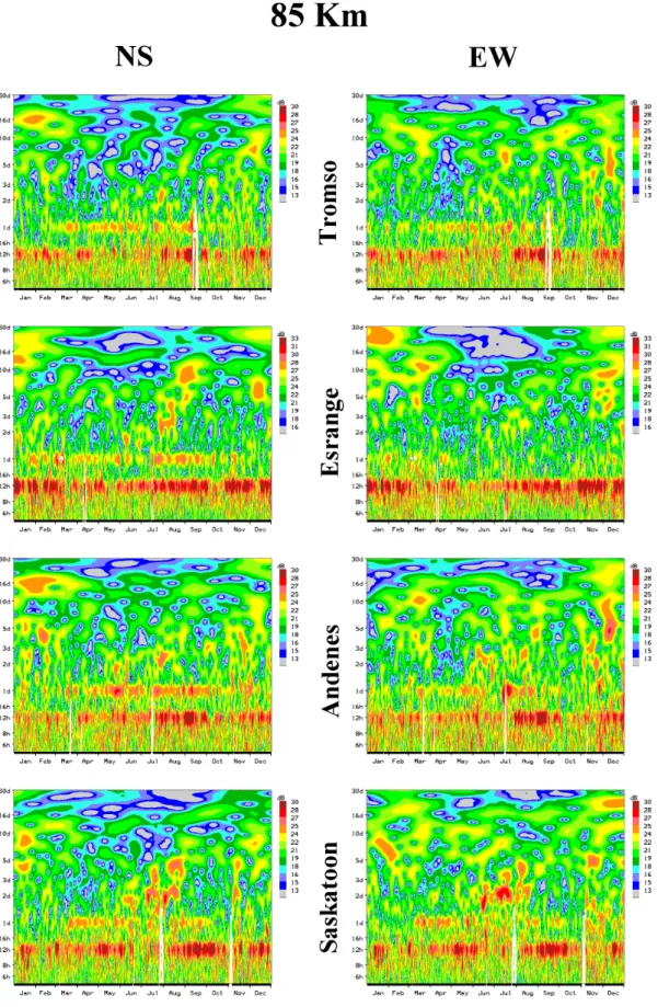
The annual contours of wavelet intensities as functions of frequency versus time, for the altitude of 85 km, and at the
three locations in Scandanavia and for Saskatoon (52◦N,
107◦W) are shown in Fig. 2. We have included the
mid-latitude location to illustrate the characteristic changes in at-mospheric waves over circa 20 degrees of latitude. The al-titude was chosen as a compromise, since at this mesopause height the tides and planetary waves (16-, 2-day) are all nor-mally present with significant amplitudes. Brief mention of
the PWs is made here, but specific discussion and figures fol-low in Sect. 6.
The spectra for the three 70◦N MLT radars are quite
sim-ilar in characteristics. For the 12-h tide and in both wind components (meridional, NS and zonal, EW) there are max-ima in the late-summer/autumn, somewhat lesser ones in winter, and perhaps increases in the spring; at Esrange the minima during October are particularly short in duration and will be clearer in the contour plots for the MLT which fol-low in Sect. 5. For the 24-h tide there are generally maxima in summer-centered months (typically March to September). There are some monthly differences already evident between Esrange and Andenes-Tromsø, which will also be well de-fined in the later multi-height contour plots, for example, the EW component at Esrange has relatively weak amplitudes in the later summer-autumn months at this altitude of 85 km. It should be noted that the Esrange contours have been moved by 3 dB, which is consistent with the earlier system com-parisons (Andenes-systems/Tromsø-MFR) which showed a speed ratio of ∼1.5. This possible bias will be discussed later in more detail. The 52◦N tidal spectra are quite similar to those at 70◦N, although the 12-h tide’s winter and spring maxima are clearer, and the 24-h tide’s maximum is reached in spring rather than summer.
The PW features of Fig. 2 are also similar at the three 70◦N MLT radars; for example, with the quasi-2-d wave hav-ing bursts of activity in summer and also in the winter months (see also Nozawa et al., 2003). Both components are in-volved. At Saskatoon the more familiar pattern of dominant activity during the summer at mesopause heights is revealed for this so-called “Rossby-gravity normal mode”. The other PWs, which have received most attention at middle latitudes, are the Rossby (normal) modes (the so-called 5, 10, 16-d waves). The ranges of observed periods associated with these are typically 5–7, 8–10, 12–22 days due to Doppler shifting by the background winds (Luo et al; 2002a, b). Indeed, in this year at 52◦N there are maxima in winter months for the 16-d PW in the EW component, and more intermittent activ-ity (occurrences of contours above 22.5 dB) between the 2-d and 16-d band. The 70◦N MLT radars have a similar pattern, but the 16- d EW amplitudes appear slightly weaker (Luo et al., 2002b), and the activity in the NS component is relatively more substantial, as will become clearer later when specific 16-d contour plots are discussed. There are also contours above the 22.5 dB level for periods of 20-30 days which have been described as “extra long period” oscillations by Luo et al. (2001). These were shown to have correlations with the solar rotation period, and to have climatologies rather simi-lar to those of the 16-d PW. Generally speaking, the occur-rences of substantial activity (contours above 22.5 dB, yellow to red) in the band from 2 to 30 days are quite similar at the three MLT radars for example, close to 16 days in January (NS); 5–10 days in December (EW), and 2 days in July (NS). However, even over scales of 125-270 km in Figure 2, the spatial-temporal intermittency noted in the North America-Pacific sector (Luo et al., 2002a, b) and in the CUJO network (Manson et al., 2003b) is evident here.
A. H. Manson et al.: Mesopause dynamics:The PSMOS-DATAR project 371
Fig. 2. Annual (2000) contours of wavelet intensities as functions of frequency versus time for the meridional and zonal (NS, EW)
compo-nents of the winds at four locations (Saskatoon, and the 3 Scandinavian-Triangle sites, Tromsø, Esrange, Andenes); the altitude is 85 km. Analysis details are provided in Sect. 2. A dB limit of 33 is used for the MWR at Esrange and 30 for the MFRs, to account for the speed-bias found earlier (Manson et al., 1992) and to allow for easier comparison of the spectral features.
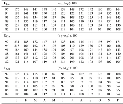
Table 1. Ratios of variances of the winds from the three MLT radars: E, Esrange; A, Andenes; T, Tromsø. The values are calculated for the
height of best correlation between the two respective data sets.
Ekm (σE/σT)x100 97 176 148 141 148 146 139 148 172 142 160 180 164 94 183 161 138 140 132 120 122 151 133 167 155 151 91 155 149 134 130 117 108 108 125 125 142 149 143 88 142 135 119 117 108 111 105 110 115 119 134 141 85 129 131 111 111 107 111 106 111 103 107 115 130 82 117 112 112 100 112 119 104 112 95 97 106 108 EKm (σE/σA) x 100 97 231 188 172 147 118 123 126 145 141 195 190 171 94 218 166 162 151 108 105 110 129 130 173 166 158 91 186 160 144 138 104 102 97 108 121 147 156 143 88 161 141 127 125 100 106 101 105 114 131 135 140 85 137 133 112 123 105 109 201 108 105 116 114 127 82 121 116 107 119 113 134 199 122 102 107 107 105 TKm (σT/σA) x 100 97 126 114 115 100 82 91 86 102 92 125 108 108 94 119 112 110 112 81 86 85 88 99 119 108 105 91 112 114 109 107 90 89 92 87 93 104 98 94 88 113 111 105 107 92 92 98 93 100 108 98 94 85 108 105 102 109 91 108 107 96 102 107 96 95 82 105 104 98 112 101 111 113 108 107 110 103 94 J F M A M J J A S O N D
4 Correlations of the Wind Field Across the Triangle: Height Calibrations and Speed Ratios
For comparisons of the contours (height versus time) of the mean wind and various wave types (tides, GW and PW) across the S-Triangle a good height calibration for each radar is highly desirable; at each system great care has been taken to optimize this process. Electronic calibrations have been used, but the use of targets at known altitudes, for example, balloons, which are the most desirable, are not yet available. Errors of 2 km are still possible between systems, as prob-lems involving uncertainties in the ground-plane for antennas can introduce errors of this magnitude.
It seems useful, however, to use the data in rather raw form, before harmonic analysis is applied to investigate the wave types and to assess the existing height calibrations. We repeat and extend analysis developed for the Canadian tri-angular array of 3 MFRs. The simplest but highly effec-tive approach was to form composite or mean-days of wind vectors (∼80–100 km) from hourly-mean values, over inter-vals of typically one month (for example, Manson and Meek, 1991a). Such plots are dominated by the tides, especially in the winter and autumn months, and show regular vector rota-tions with time at particular heights, and with heights (3 km intervals) at particular times. For the Canadian-Triangle such plots were extremely similar at the 500-km spacings, and “pattern recognition” showed the highest correlations of time sequences to be at identical gated-heights, i.e. the height
calibrations were correct to better than 3 km, assuming no tilt of the atmosphere or of dynamic processes.
Composite days were formed for the MLT radars of the S-Triangle during a winter month (January), when the 12-h tide provided clear temporal rotation of the vectors and also phase-progression with height. (The 2-hour means available were spaced by 1 h.) Instantaneous or common UT, values were used. The wind and wave patterns were very simi-lar, but from careful inspection, differences in heights for the highest correlations (similarity) of vector time sequences emerged. Winds for a height gate h (km) at Esrange were most similar to those at (h or h-3) at Tromsø and at (h or h+2) at Andenes.
A quantitative analysis was developed for the wind vec-tor comparisons, which provided correlations between the twelve monthly time-sequences of 2-hour means for any radar-pair, and for all heights (circa 80-100 km). The method involves complex (i.e.wind vector) cross correlations, and se-lection of the height-pair with maximum correlation. These results confirmed the method of visual inspection and pro-vided a full year of analysis. Taking the median differences, as there were no trends with height or month, values at height gate (h) at Esrange were most highly correlated with (h-1.5) at Tromsø and (h +2) at Andenes. These are small factors and consistent with possible real uncertainties in absolute height calibrations.
There is, however, a final consideration, when comparing
A. H. Manson et al.: Mesopause dynamics:The PSMOS-DATAR project 373
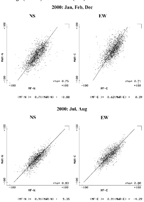
Fig. 3. Plots of wind-components (EW, zonal and NS, meridional) for the Meteor Winds Radar (MWR, Esrange) versus the Medium
Frequency Radar (MF, Tromsø): the height of 88 km is shown for the winter (January, February and December) and summer (June, July and August). The lines of best fit (least-squares) are shown, as are the equations (with slope and offset) of these lines. Correlations (rho) are also provided.
longitude (Fig. 1). There will be a phase (angle) difference for the vectors, depending upon the migrating tide. Because of this factor, and the vector-angle changes with height due to the dominant tide, both the composite day and correlation, analyses will show a small offset in heights of maximum correlation even when the radars are perfectly calibrated: the relation is approximately (h) Esrange = (h+1)Tromsø = (h+2)Andenes. When compared with the relation for height differences using the correlation method, this shows that the height calibrations for Esrange and Andenes are probably
correct, and that the Tromsø values of h should be increased by circa 3 km.
With this result available, subsequent analyses can proceed in two ways. Harmonic and spectral analysis can be applied and contour plots formed (Sect. 2) using gated heights for Tromsø, modified or corrected by the modest but still signif-icant factor just determined. At first thought this should pro-duce greater similarity of climatological features (in height) than without such intervention. Indeed, it is the case that mean-wind and tidal contours formed without “correction”
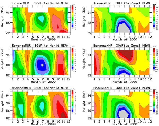
Fig. 4. Annual (2000) contours of the EW (zonal) and NS (meridional) components of the mean winds, as functions of height versus time:
plots for Tromsø, Esrange and Andenes are shown. Data from Tromsø are shown for a height-range lower by 3 km to enhance the similarities of contours/colours. This is consistent with the height calibration discussion of Sect. 2.
(below in Sect. 5) do show small altitudinal differences con-sistent with those factors just determined. On the other hand, the method used does not prove that the height calibration for the Tromsø MFR is in error by 3 km. There could be com-plex dynamical processes, local to each MLT radar, which produce this difference. And since this paper is focussed on a comparison of the winds from three radars at spaced loca-tions we argue to retain the experimentally calculated height calibrations.
However, we show an extra 3 km of data for Tromsø that will be found to provide better visual agreement of contours and “colours”, and perhaps a persuasive argument that such a correction is appropriate. It is also consistent with the more limited radar height comparisons carried out during the PMSE observations of 1994 (Bremer et al., 1996).
While dealing with the 2-hour means (at common UT) there was the opportunity to compare the wind components from the two radar types. In Fig. 3 we show such plots for Esrange (MWR) and Tromsø (MFR) during the winter (January, February, December, 2000) and summer (July, Au-gust) months at 88 km. Plots for both wind components are shown. Based upon the slopes of these lines for the sum-mer, and the histograms of vector-angle differences that were also produced (not shown), best agreement between the data
sets occurred when there was no height difference between the systems (3 km were assessed also). This is consistent with the vector-correlation method, where only a 1.5-km off-set ((h)Esrange = (h-1.5)Tromsø) was found. For the win-ter, when the tidal oscillations are stronger (Sect. 5), the his-tograms indicated best agreement for an interpolated 1-km difference in the gated heights. The data are close to the lines of best-fit, indicating good quality data with high correlations (the correlation coefficients are also on the figure).
The slopes of the lines of best-fit differ between seasons: MWR/MFR is 1.41–1.61 in winter, and 1.1 in summer. This is the first time that seasonal differences have been reported, and we have no explanation for this. The calculation was repeated for 2001, and ratios of 1.33–1.39 and 1.19–1.14 respectively, were obtained. The ratios are similar to those found earlier (Manson et al., 1992) for the Andenes systems compared with the Tromsø MFR (1.54).
The correlation analysis used for the height comparisons were also used to show the height and monthly variation in the speed differences. The total variances (NS, EW) have been formed and ratios calculated for the Tromsø-Andenes MFR pair (σ T /σ A), the Esrange (MWR)-Andenes (MFR) pair (σ E/σ A), and the Esrange-Tromsø pair (σ E/σ T ) (Ta-ble 1). The variances will be dominated by tidal winds.
A. H. Manson et al.: Mesopause dynamics:The PSMOS-DATAR project 375
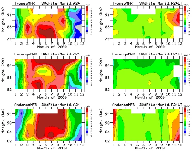
Fig. 5. Annual (2000) contours of the NS (meridional) component of the semi-diurnal tidal amplitudes (A12) and phases (P12LT; local solar
times), as functions of height versus time: plots for Tromsø, Esrange and Andenes are shown. The times are for the maximum tidal wind in the northward direction. Tromsø data are again shown for a height interval lower by 3 km.
The Tromsø winds are modestly larger than Andenes (5% median) and there is a seasonal change (Tromsø values are larger/smaller in winter/summer). Ratios for the Esrange-Andenes and Esrange-Tromsø pairs show the Esrange winds to be generally relatively larger than those for the two MFRs. As expected, the variance ratios at 88 km for Esrange-Tromsø are very similar to the values obtained from Fig. 3. The surprising result is that the ratios for both comparisons with Esrange in Table 1 vary with month (smaller in sum-mer than in winter) and with height (increasing with height usually). Median values (MWR/MFR) are 1.57 at 97 km and 1.1 at 85 km. We have been unable to find a reason for these results.
5 Mean Winds and Tides
The annual contours of the EW (zonal) and NS (meridional) components of the mean winds, as functions of height versus time, are shown in Fig. 4. The height co-ordinates are dif-ferent at Andenes due to the 2-km data-sampling. Also, we show Tromsø data from 79–94 km (original height calibra-tion) for reasons of gaining colour/contour similarities with the other MLTs; if the 3-km height correction of Sect. 3 were
then applied, the height range of the data would be the same for the three radars.
The zonal mean contours are then very similar in posi-tion and strength, except for the strong summer eastward cell above 90 km at Esrange. These are the altitudes that cannot be reached by the MF radar pulses without significant group-retardation or total reflection (Sect. 2). The heights of re-versal of the EW flow are near 90 km at all MLT radars; An-denes (92 km), Tromsø (90+3=93 km), Esrange (89 km). The slightly lower height for Esrange is consistent with the ex-pected latitudinal trend. The structure/colours of the merid-ional (NS) contours are also very similar; the speeds are much lower than for the EW and so contours may change, dependent upon small differences in the wind vectors across the S-Triangle. In particular, in summer, the southward flow at Esrange is stronger for longer duration over more altitudes; and this is also true for heights below 90 km, where the EW winds are very similar in magnitude to the other locations.
The contours of Fig. 4 do show larger variability of shape
and position than do similar contour plots from the 50◦N
Canadian Triangle (not shown). This may be a regional ef-fect, as the 70◦N Triangle is in mountainous country rela-tively near to the ocean. Possible physical processes are dis-cussed in the Conclusion.
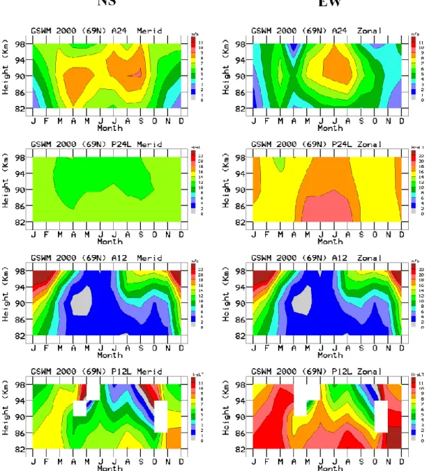
Fig. 6. GSWM-2000 (Global Scale Wave Model, year 2000 version): annual contour plots of the NS (meridional) and EW (zonal)
compo-nents of the diurnal and semidiurnal tidal amplitudes (A24, A12) and phases (P24LT, P12LT; local solar times), as functions of height versus time, for the latitude (69◦N) nearest to the radars of the Scandanavian Triangle are shown. The times are for the maximum tidal wind in the northward and eastward directions.
The annual contours of the amplitudes and phases of the semi diurnal (12-h) tide are provided in Fig. 5: the merid-ional (NS) component is chosen, as the zonal portrays the same features but with the phases being closely in quadra-ture, as expected. The phases are appropriate to the local (solar) times at each radar location. Contours for amplitudes and phases are generally similar to those shown for the first
time at 70◦N (Tromsø) by Manson and Meek (1991b). Tidal
contours from Esrange have also been shown for the first six
months of 2000 by Mitchell et al. (2002), and those essen-tially agree with the plots shown here. We focus first upon the strong similarities between the tidal oscillations observed by the three MLT radars: there are clear transitions in phases and phase-gradients between winter (wavelengths λ ∼ 50 km) and early summer (λ > 100 km); there are dominant late summer-autumn amplitude features, beginning at higher alti-tudes in June and maximizing near 90 km in September; there are very modest changes in phase during the development of
A. H. Manson et al.: Mesopause dynamics:The PSMOS-DATAR project 377
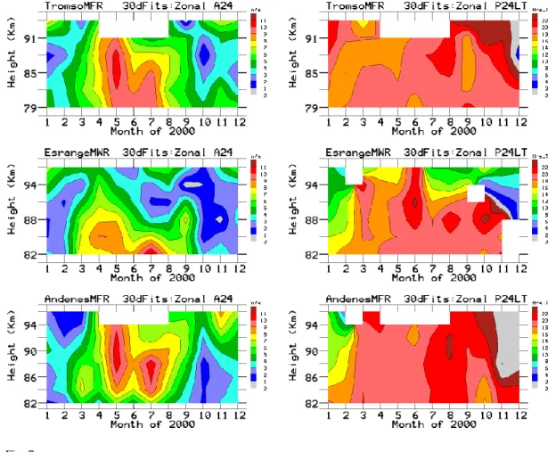
Fig. 7a. Annual (2000) contours for the (a) NS (meridional) and (b) EW (zonal) components of the diurnal tidal amplitudes (A24) and phases
(P24LT; local solar times), as functions of height versus time: plots for Tromsø (3 km height interval difference), Esrange and Andenes are shown. The times are for the maximum tidal wind in the northward and eastward disrections.
this feature; and the largest temporal changes in phase occur in October, between the autumn amplitude maxima and the developing maxima of the winter solstice.
There are also interesting differences between the 12-h tidal amplitudes (Fig. 5) for the three locations. First, the similarities between Andenes and Tromsø features are en-hanced by the +3 km adjustment in height gates for Tromsø, as discussed earlier. Secondly, the amplitudes of the tide at Esrange are clearly greater above 88 km than at the other lo-cations, consistent with the “scatter plots” of Fig. 3 and Ta-ble 1 of Sect. 3. This affects the structure/colours of the au-tumn maxima and especially the winter solstice maxima
(Es-range/Tromsø, amplitudes ∼= 1.4). However, there are also
differences between MFR locations, as although their au-tumn features are very similar and strong (> 20 m/s), the An-denes amplitudes in winter (January) are much weaker than at Tromsø (Tromsø/Andenes ∼=1.5). (These differences exist in the EW component also). The changes in contours asso-ciated with variations of analysis at any site, for example, by using un-weighted hourly values (Sect. 2), are smaller than the differences noted between the three MLT radars. It is not possible to determine whether the changes between Tromsø and Andenes are related to MFR antenna-system differences, but the experience with the Canadian-Triangle suggests that
this is not a significant issue as far as the tides are concerned. It should also be noted that the latitudinal tidal studies in-volving Tromsø (Manson et al., 1999b, 2002b) have shown significant inter-annual variability at Tromsø, as well as dif-ferences between EW and NS components in some years.
We include a figure using the GSWM-2000 (Global Scale Wave Model, year 2000 version; Hagan et al., 1999; Man-son et al., 2002b), for compariMan-son purposes (Fig. 6). The winter phase-contours for the 12-h tide, along with their ver-tical gradients, agree well with those observed at the three sites for both NS and EW components; and the observed strong phase gradients of October are shown by GSWM-2000. However, the modelled vertical phase-gradients from April-September differ substantially, with unobserved wave-lengths of ∼30 km. The amplitude contours of the model show a strong winter maximum, similar in absolute terms to Esrange, but there is only a modest maximum at the upper levels centred on September. Otherwise, the amplitudes are much weaker (factors of near 2) than observed by the MLT radars. Possible reasons for the differences between mod-elled and observed tides are discussed in the Conclusions. It is certainly valuable to conduct comparisons of such contour plots at specific locations, as this is the most demanding test of the model; tidal differences are not as evident in the
lati-Fig. 7b. See lati-Fig. 7a.
tudinal plots of various types which have been used in other studies, for example, Manson et al. 2002b.
A brief comment on the differences between the 12-h tidal characteristics at 70◦N and mid-latitudes (40 − 52◦N) is ap-propriate (Manson et al., 2003a). The amplitude contours of the latter are also dominated by the winter and late summer-autumn peaks, although these latter are restricted to August and September. Amplitudes in these peaks are somewhat larger (factors of 1–2) than at 70◦N, as also shown by Man-son et al. (2002b). The phase structures and gradients are quite similar at high and middle latitudes, suggesting simi-lar mode composition. Finally, the amplitude-phase contours for the 50◦N Canadian-Triangle (not shown) do demonstrate
slightly less variability with height and time over 500 km than do, say, those of the Andenes-Tromsø MFR pair. This is also discussed in the Conclusions.
The annual contours for the amplitudes and phases of the diurnal (24-h) tide are provided in Figs. 7a, b: both of the components are shown, as although they portray simi-lar broad seasonal features, there are significant differences within the summer-centred months. The amplitudes of this tide are approximately half those of the 12-h tide (note that the maximum contour level is 11 m/s rather than 22 m/s). Contours for the amplitudes and phases are generally sim-ilar to those shown originally for Tromsø by Manson and Meek (1991b). We focus again first upon the strong
simi-larities in EW and NS oscillations seen by the three MLT radars: the amplitudes are largest in a broad feature from March to September, for which the phases evidence generally small vertical gradients; and the vertical phase gradients are stronger in the winter months. It is not obvious that the +3 km adjustment in the height-gates for Tromsø enhances the simi-larities between locations in this case, due to the greater vari-ability in this tide.
Considering now the component differences for March un-til September, there are consistent decreases in amplitude with increasing height for the EW component (Fig. 7b), es-pecially in mid to late summer, which contrasts with the
NS component (Fig. 7a). The phase gradients are often
larger and more irregular in the regions of small EW am-plitude (Esrange and Tromsø). Such features may be due to small tidal signals. There are interesting differences be-tween the contour plots for the three locations, and for each of the components. Again, the changes in contours at any site, associated with variations in analysis, for example, us-ing unweighted hourly values (Sect. 2), are smaller than those between the MLT radars. Considering the NS com-ponent contours (Fig. 7a), the amplitude structures in the summer-centred months differ at each location, so there is no consistency in the amplitude ratios between locations; and the phases at Tromsø and Andenes are very similar in the non-winter months throughout the MLT region, while
Es-A. H. Manson et al.: Mesopause dynamics:The PSMOS-DATAR project 379 0 5 9 13 Amplitude (m/s)
Tromso (70N,19E) 2000 EW 16-d & BGW
Jan Feb Mar Apr May Jun Jul Aug Sep Oct Nov Dec 70 75 80 85 90 95 Height (km) 10 10 10 10 -20
Tromso (70N,19E) 2000 NS 16-d & BGW
Jan Feb Mar Apr May Jun Jul Aug Sep Oct Nov Dec 70 75 80 85 90 95 5 0 5 9 13 Amplitude (m/s)
EsrangeMWR (69N,21E) 2000 EW 16-d & BGW
Jan Feb Mar Apr May Jun Jul Aug Sep Oct Nov Dec 70 75 80 85 90 95 Height (km) 10 10 10 10 -20 EsrangeMWR (69N,21E) 2000 NS 16-d & BGW
Jan Feb Mar Apr May Jun Jul Aug Sep Oct Nov Dec 70 75 80 85 90 95 5 -10 0 5 9 13 Amplitude (m/s)
Andenes (69N,16E) 2000 EW 16-d & BGW
Jan Feb Mar Apr May Jun Jul Aug Sep Oct Nov Dec 70 75 80 85 90 95 Height (km) 10 10 10 10 -20
Andenes (69N,16E) 2000 NS 16-d & BGW
Jan Feb Mar Apr May Jun Jul Aug Sep Oct Nov Dec 70 75 80 85 90 95 5
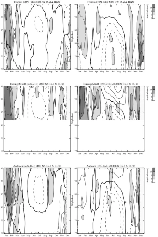
Fig. 8. Annual contours of wave amplitudes for the meridional and zonal (NS, EW) components of the 16-d PW, as functions of height
versus time: plots for Tromsø, Esrange and Andenes are shown. The background-mean winds (BGW) are shown by the use of continuous (eastward, northward) or dashed lines (westward, southward). Analysis details are provided in Sect. 2.
range shows a small but consistent vertical gradient above 90 km. Finally, for the EW component (Fig. 7b), there is general similarity of the rather complex amplitude contours, although the amplitudes at Esrange in July–November are clearly the smallest. Regarding phases, there are months when any one pair of radars evidence very similar contour structures and gradients for example, phases at Esrange and Andenes in January–February.
Comparing with GSWM-2000 (Fig. 6), the model also has summer maxima, but the height-time structures of the con-tours differ significantly from the observations. However, the peak-amplitudes (∼ 10 m/s) are similar, and the NS con-tours do show enhanced values over an extended interval from spring to autumn, which is similar to the observations. Regarding phases, the absolute values for the EW component (14–20 h) are similar to observations, but the phase structures
and gradients differ; and for the NS component the phase val-ues (10–14 h) and their gradients are very similar in the non-winter months. The vertical phase gradients of both compo-nents do not show the observed tendency for larger values in the winter. It must be reiterated that GSWM is a 2-D model, and the non-migrating tidal modes so evident from global satellite analysis (Manson et al., 2002a, 2004b) will typically lead to local observations, such as those for the S-Triangle, being different from the model.
Commenting now on the differences in 24-h tidal charac-teristics at 70◦N and mid-latitudes (40 − 52◦N), the
ampli-tude contours of the latter are dominated by late summer and autumn, and late winter-spring peaks; and the absolute val-ues decrease strongly from Platteville to Saskatoon and then to the S-Triangle (Manson et al., 2002b, 2003a). The phase structures also differ, with the high latitude dominance of the evanescent mode (S(1,-1)) being modified at mid-latitudes by the propagating mode (e.g., S(1,1)). This is especially ev-ident in winter, when relatively short wavelength structures (∼ 50 km) may occur. Finally, the amplitude-phase contours
for the 50◦N Canadian Triangle (not shown) demonstrate
slightly less variability with height and time over 500 km than do those of the Scandinavian-Triangle; but for both lo-cations the variability of the 24-h tidal oscillations is signifi-cantly greater than that of the 12-h tidal oscillations.
6 Planetary waves
6.1 16-d PW
The annual contours of wave amplitudes for the EW and NS components, as functions of height versus time, over the Scandanavian-Triangle are shown in Fig. 8. The background-mean winds (BGW) for the 48-day window (Sect. 2.2) are also shown. The relative amplitudes within the MLT region and across the S-Triangle are consistent with the spectra of Fig. 2: the NS amplitudes often dominate the EW; the wave activity (amplitudes above 5 m/s) is largest in winter-centred months; and the wave activity is restricted to mesopause heights (∼80 km) in summer.
Considering Fig. 8 in more detail, the 16-d PW activity (NS) in winter extends throughout the MLT (70-95 km). The greater range of data obtained from the MFRs in the meso-sphere (70-82 km) is also very evident (the tidal figures of the previous section could also have shown some data at these heights, but the emphasis there was upon comparative clima-tologies). There are two substantial bursts of activity centred especially on January–February and to a weaker extent in De-cember at all three stations; the Jan.–Feb. event is strong in the NS component at the three radars, while there is activ-ity at Esrange and Tromsø but not at Andenes for the EW component. The amplitudes are largest at Esrange, but this is likely to be mainly due to the speed bias discussed in Sect. 2. Otherwise some of the variations of wave activity in the first “grey scale” of 5–9 m/s, especially in the summer, are
pos-sibly associated with noise, as amplitudes of circa 5 m/s are usually at the 90% significance level (Luo et al., 2000.)
The recent studies of this wave (Luo et al., 2002a, b) noted its spatial and temporal intermittency, with bursts of activity occurring at different times at the MFR locations:
Tromsø (70◦N, 19◦E), Saskatoon (52◦N, 107◦W),
Lon-don (43◦N, 81◦W), Hawaii (22◦N, 160◦E), Christmas Is-land (2◦N, 157◦E). Also, results from UARS-HRDI (Luo et al., 2002b), which were based upon hemispheric wave mode (m=1) fits, showed strong latitudinal restrictions in the bursts of activity. Theoretically, this wave is expected to propa-gate from the lower atmosphere and through the eastward flow of the winter hemisphere, with the possibility of sum-mer mesopause activity due to propagation from the winter hemisphere. The results from the 2-D Global Scale Wave Model (GSWM) in Luo et al., (2000, 2002b) were generally consistent with this simple scenario, but also demonstrated strong sensitivity to the background winds in the model, for example, strong winter winds can lead to the so-called “crit-ical velocity” of Charney and Drazin (1961) being exceeded, the refractive index becoming smaller, and wave propagation being minimized. Also, Hagan et al. (1993) very nicely ad-dress the issue of intermittency for planetary waves. They note that variations of the relative magnitudes of the summer and winter “jets” on time scales of weeks could account for the intermittency; and that the resonant period of the wave is sensitive to these changes in the “jets”. Such effects would be associated with the propagation of both 16- and 2-d PWs, and lead to their observed interannual variability.
The latitudinal plots of Luo et al. (2002b) showed that above 82 km the observed EW amplitudes for 1993-5 were
comparable at 52◦N (Saskatoon) and 70◦N (Tromsø), and
that the observed and modelled (GSWM) NS amplitudes were comparable or greater than the EW amplitudes at 70◦N. Our present results are consistent with these earlier studies.
6.2 2-d PW
The annual contours of wave amplitudes for the 2-d PW at the three MLT radars are shown in Fig. 9; the same format as Fig. 8 has been used. Despite the considerable number of studies of this wave type over the last two decades (for example, Meek et al., 1996; Thayaparan et al., 1997), con-tour plots of this type have not been widely used. Emphasis has been placed upon the bursts of activity during summer months (July-August in the N.H.) at mesopause heights. In that context we note the modest summer mesopause activity (amplitudes 6–8 m/s) in both EW and NS components at all three MLT radars; the strongest burst is at the end of July in the NS component, when amplitudes exceed 10 m/s. How-ever, the general level of activity at 70◦N is much lower than
at 40 − 52◦N (Manson et al., 2003a, 2004a), where bursts
occur from June to August.
Of greater note is the modest but consistent winter activity that can be seen throughout the MLT at all stations. Nozawa et al. (2003), using Tromsø MFR and EISCAT observations, have studied these winter waves in some detail. The winter
A. H. Manson et al.: Mesopause dynamics:The PSMOS-DATAR project 381 0 6 8 10 Amplitude (m/s)
Tromso (70N,19E) 2000 EW 2-d & BGW
Jan Feb Mar Apr May Jun Jul Aug Sep Oct Nov Dec 70 75 80 85 90 95 Height (km) 10 10 10 10 10 -20 -30 -30 Tromso (70N,19E) 2000 NS 2-d & BGW
Jan Feb Mar Apr May Jun Jul Aug Sep Oct Nov Dec 70 75 80 85 90 95 5 5 5 0 6 8 10 Amplitude (m/s)
EsrangeMWR (69N,21E) 2000 EW 2-d & BGW
Jan Feb Mar Apr May Jun Jul Aug Sep Oct Nov Dec 70 75 80 85 90 95 Height (km) 10 10 10 10 10 -20 EsrangeMWR (69N,21E) 2000 NS 2-d & BGW
Jan Feb Mar Apr May Jun Jul Aug Sep Oct Nov Dec 70 75 80 85 90 95 5 5 -10 -10 -10 0 6 8 10 Amplitude (m/s)
Andenes (69N,16E) 2000 EW 2-d & BGW
Jan Feb Mar Apr May Jun Jul Aug Sep Oct Nov Dec 70 75 80 85 90 95 Height (km) 10 10 10 10 10 -20 Andenes (69N,16E) 2000 NS 2-d & BGW
Jan Feb Mar Apr May Jun Jul Aug Sep Oct Nov Dec 70 75 80 85 90 95 5 5 5 5 5 5
Fig. 9. Annual contours of wave amplitudes for the zonal and meridional (EW, NS) components of the 2-d PW, as functions of height
versus time: plots for Tromsø, Esrange and Andenes are shown. The background-mean winds are shown by the use of continuous (eastward, northward) or dashed (westward, southward) lines. Analysis details are provided in Sect. 2.
activity is also very clear and even stronger at 40 − 52◦N (Manson et al., 2003a, 2004a), and the absence of an earlier study of the winter wave has to be a minor embarrassment to the community.
Theoretically, the behaviour of the 2-d PW is consistent with the discussion above on the 16-d PW. However, in contrast to the 16-d PW, the faster moving (wave numbers,
m = 3 or 4 are typical) 2-d wave does not experience a
critical level in the summer mesospheric westward flow, and achieves significant amplitudes (Hagan et al., 1993, Figs. 2, 4, 6) at mesopause heights (85–90 km) and at middle to high latitudes. (Maximum responses are between the equator and
±30◦.) In winter the eastward flow leads to larger intrinsic phase speeds, and the so-called “critical velocity” (Charney
Fig. 10. Variances of the winds from the 2-6 hour band-pass filter, as a function of azimuth, for two height layers, from the three MLT radars
of the Scandinavian-Triangle: scales for the intensities and the orientation are shown. The resulting “perturbation ovals” are shown in pairs for ease of comparison.
and Drazin, 1961; Luo, 2002c), that is a function of both phase speed and wave number, is smaller for the 2-d wave (than for the 16-d PW) and rather more easily exceeded. Hence, the amplitudes of this wave are expected to be smaller in winter, as Hagan et al. (1993) demonstrate. This modest solstitial difference in the GSWM’s response has been over-stated, however, by interpreters of this paper, as the results
here (and at 40 − 52◦N, by the CUJO network, Manson et
al., 2003a, 2004a) show substantial winter amplitudes.
7 Gravity Waves
As described in Sect. 2, a band-pass filter has been applied to the winds’ time-sequences, to allow for an assessment of GW intensities and directional properties in the 2-6 h band
(Fig. 10). Earlier studies have involved these
“perturba-tion ovals” (years 1993/4) in the Canadian prairies over the
500 km triangle (Manson et al., 1997), and from 2–70◦N
(Manson et al., 1999a). In that context there are no sur-prises in Fig. 10: the sizes of the ovals follow semi-annual oscillations (SAO) at 76–88/82–88 km, and annual oscilla-tions at the 61–73 km layer. The orientaoscilla-tions of the ovals at the upper layer are interesting; they are more zonal at An-denes, while at Esrange and Tromsø there are more months
when the meridional direction is preferred. The amplitudes are quite similar across the S-Triangle, although except for the summer months the Esrange ovals are somewhat larger than at the other two locations. This, and the tendency for the Esrange ovals to be more meridionally orientated, could be associated with the distribution of meteor trails within the antenna beams. The large area involved with the distribution of these trails (Sect. 2, circa 500km) will also tend to increase the variance compared with the MFR systems (for example, Nakamura et al., 2002). Otherwise, the reasonable agreement between the Tromsø and Esrange ovals (compared with other radar comparisons we have done) is pleasing, given that an MWR has not been used for this analysis before.
It is useful to compare the spatial variations over the S-Triangle with those noted over the 500 km MFR Canadian-Triangle. For the latter, very modest changes in perturba-tion oval size and orientaperturba-tion were noted between the purely east-west pair of Saskatoon and Sylvan Lake radars. The Tromsø-Andenes MFR pair in Fig. 10 clearly demonstrates more directional variability. However, for the Saskatoon-Robsart MFR pair, where Saskatoon-Robsart is located 500 km south-west, strong directional changes (often as much as 90 de-grees, and more zonal than meridional) were observed. Also, Robsart ovals were modestly larger. In that context the dif-ferences between the ovals of Tromsø and Esrange, two
loca-A. H. Manson et al.: Mesopause dynamics:The PSMOS-DATAR project 383 tions that are really quite similarly spaced, are qualitatively
similar to the Canadian pair.
Our earlier studies using 1993/4 data (Manson et al., 1999a) had shown that the GW intensities (ovals) were sur-prisingly large in the Tromsø area, comfortably exceeding the Saskatoon values. We have assessed the years 1998-2001 and while there were some very large summer months in 1998 and 1999, during 2000 and 2001 the Tromsø MFR ovals were generally smaller than those for Saskatoon. It is, therefore, clear that interannual variability is a significant factor with this GW characteristic. It is also clear that our ear-lier suggestion that the intensities are large across the entire northern Scandinavian region was based upon insufficient ev-idence. The mountainous nature of the region and its proxim-ity to the ocean and to changing weather patterns are possible explanations for the large inter annual variability, and indeed the spatial variability (Tromsø-Andenes), which has also just been noted.
The reasons for changes in oval characteristics, both in size and in orientation, are clearly complex, and involve both sources and propagation conditions. Assessment of ovals from GCMs is, therefore, useful and our study of CMAM (Manson et al., 2002c) included the 2–6 h band. More work of this nature is called for.
We make only brief comments about the possibilities for other GW analyses. There was relevant discussion already in the Introduction regarding the results of such GW analyses for the 500 km Canadian Triangle. Given the smaller size of the S-Triangle there were grounds for cautious optimism that a larger number of GW would be resolved and characterized. Time-sequences of daily values from the 2–6 h band-pass filter were prepared for each radar location and for three height layers: 82–85, 88–91, 94–97 km. For each layer there were 15–20 days over the full year when significant peaks of variance were noted at each of the three MLT radars. How-ever, these peaks were noted to exist over two neighbouring height-layers on only six instances, and the peaks were com-mon to the three layers in only one instance. This horizon-tal uniformity, along with limited vertical correlation, is very similar to the GW-related characteristics noted for the Cana-dian Triangle (Hall et al., 1995a, b). A hodograph analysis, similar to that used in the earlier studies, will, therefore, be applied to these data in the future.
8 Conclusions
The existence of the three MLT radars in the Scandinavian-Triangle has provided a unique opportunity both to compare systems and to assess the variability of all the atmospheric wave types over distances of 125–270 km. Correlation tech-niques provided an independent method of height calibration for the radars, and inferred that the Tromsø radar data re-quired a +3 km adjustment for best agreement of the tidal winds across the Triangle. That analysis also allowed for wind (mainly tidal) speed comparisons: the Tromsø values are modestly larger (5%) than those at Andenes, a difference
consistent with different versions of the FCA winds analysis and possible differences in antenna systems; and the Esrange values are larger than those at the MFR sites (median annual factors of 1.6 at 97 km, 1.1 at 85 km). The variation of ratio with season (smaller in summer) and with height (82–97 km with 3 km sampling) is a new result, and likely holds clues as to the reasons for this effect.
Annual contour plots for the winds, and for tidal ampli-tudes and phases, throughout the MLT region show strong similarities between the three radars of the S-Triangle(125-270 km spacings). However, the variability of shape and po-sition of the contours is modestly larger than for the larger (500 km) Canadian Triangle of MFRs. This may be due to the proximity of this mountainous region to the Atlantic Ocean, from whence weather systems and related GW inter-actions and momentum deposition may lead to MLT dynam-ical variability, for example, Manson et al., 2002a, c. In the first of these papers, the smallest scale of global tidal lon-gitudinal variability was shown to be comparable to that of the S-Triangle; and in the second the role of GW associated with orography was shown to be important in a high resolu-tion General Circularesolu-tion Model. There have also been num-bers of theoretical studies (for example, Walterscheid, 1981; Zhong et al., 1995; Eckermann and Marks, 1996) which have explored the mechanisms by which variability of the harmon-ics (12–24 h) of the wind can be caused by GW interactions with the background wind. Here we have demonstrated a sig-nificant variation of GW activity across the S-Triangle. Most recently, Riggin et al. (2003) have discussed and studied the variability of high-latitude tides, and demonstrated the im-portance of the background winds and temperatures in re-fracting the semi-diurnal tide; there will be a regional scale of variability associated with this process.
The semi-diurnal tide has a climatology very similar to that at middle-latitudes, for example, strong transitions be-tween summer (long wavelength) and winter (short wave-lengths), but the amplitudes at times of maxima, for exam-ple, autumn, are smaller by factors of 1–2. The GSWM shows useful agreements with the MLT radars, but its sum-mer vertical phase-gradients are much larger and the autumn amplitude maximum is too weak. The contour plots for the diurnal tide (24-h) reveal that the amplitudes are about half the size of the 12-h tide; the amplitudes are largest in non-winter months, when the wavelengths are very large; and the wavelengths are smaller in winter. The GSWM-2000 also has a summer maximum, and the peak amplitudes and ab-solute values of the phases near 85 km are very similar to those observed. However, the rather complex height-time structures of the observed contours, which show considerable agreement between the three S-Triangle radars, are not repro-duced by the mode, i.e., there is no indication of the observed shorter winter wavelengths. There are also strong observed tidal differences with those at middle-latitudes (cf. Manson et al., 2002b, 2003a) where amplitudes are larger and max-ima occur closer to the equinoxes, reflecting the more impor-tant role of the S(1,1) mode. The non-migrating tidal modes (e.g. Manson et al., 2002a, 2004b), will contribute
signifi-cantly to the detailed differences between the GSWM-2000 and the tides over the S-Triangle.
These detailed assessments of the Arctic tides, using con-tour plots with observed and modelled data, are a very use-ful addition to latitudinal studies (for example, Manson et al., 2002b, c) which necessarily give less insight into the lo-cal and individual characteristics throughout the MLT region. Studies of tides remain one of the most important themes of middle atmosphere dynamics: their structure and character-istics at MLT heights depend upon forcing from global ozone and water vapour distributions in the lower atmosphere, mid-dle atmosphere wind and temperature fields and gradients, gravity wave influences through eddy diffusion and momen-tum depositions, and other wave interactions, for example, Hagan, 1996; Riggin et al., 2003; Manson et al., 2002c, 2004b). Thus, successful global modelling of the tides would indicate profoundly substantial knowledge and understand-ing of the chemical, thermal and dynamical state of the mid-dle atmosphere, including the MLT. In this regard, global ozone data of significantly improved seasonal, altitudinal, latitudinal and longitudinal distribution are becoming avail-abl, for example, Murtagh et al., 2002. Given the impor-tance of ozone-forcing for both diurnal and semidiurnal tides (Hagan, 1996), the incorporation of these new data into tidal models, such as GSWM, and even Global Circulation Mod-els through data assimilation, are likely to provide tides in better agreement with observations.
The climatologies of the high-latitude PW have been shown to differ significantly from those at middle-latitudes. For the 16-d PW, although the EW amplitudes during the maxima of winter activity are similar in magnitude to those for the lower latitudes, the NS components on occasion dom-inate the EW over the S-Triangle. Modest, but still statisti-cally significant, differences between the contour plots for the three radars again indicate the spatial and temporal inter-mittency of the local wind oscillations associated with these global-scale PW structures (Luo et al., 2002a, b). This, again, may be associated with variations of GW activity across the S-Triangle. The 2-d PW activity across the Triangle is quite coherent, but the summer amplitudes and general activity throughout the year are, respectively, smaller and less than at middle latitudes. Winter activity (EW>NS amplitudes) is actually greater than in summer (EW<NS), a fact that is only now receiving proper attention, for example, Nozawa et al. (2003). The annual contour plots for the MLT region pro-vided here put this seasonal activity of PW into even clearer context. This pattern of seasonal activity is also very clear at middle-latitudes (Manson et al., 2003a, b), which again is a surprise to those content with studying the summer man-ifestation of this “quasi-two day PW”. Given the impor-tance of interactions between PW and GW (Manson et al., 2003b; McLandress and McFarlane, 1993), and the role of PW in producing non-migrating tides (e.g. Hagan and Roble, 2001), improved understanding and modelling of PW activ-ity at Arctic latitudes is very desirable.
In conclusion, the monthly presentation of GW variances in the form of “perturbation ovals”, which provide
ampli-tudes as functions of azimuthal directions, have illustrated that the seasonal trends of the variances are quite consistent across the S-Triangle (this is the first time that such analy-sis has been applied to the MWR data), and that annual and semiannual oscillations (solstitial minima) are strong. How-ever, the GW variances and oval orientations do evidence considerable spatial and interannual variability, when com-pared with those of the Canadian Prairies. Hence, and due to the interactions of GW with tides and planetary waves, we suggest an important role for these waves in the overall dynamics of the Scandinavian Arctic.
Acknowledgements. The scientists gratefully acknowledge grants
from their national agencies (NSERC in Canada). The first authors (Manson, Meek) also acknowledge support from the University of Saskatchewan, and the Institute of Space and Atmospheric Studies. Topical Editor Ulf-Peter Hoppe thanks two referees for their help in evaluating this paper.
References
Bremer, J., Hoffmann, P., Manson, A. H., Meek, C. E., Ruster, R., and Singer, W.: PMSE observations at three different frequencies in northern Europe during the summer 1994, Ann. Geophysicae 14, 1317–1327, 1996.
Briggs, B. H.: The analysis of spaced sensor records by correlation techniques, Handbook for MAP, Vol. 13. SCOSTEP, University of Illinois, Urbana, 166- 186, 1984.
Charney, J.G. and Drazin, P.G.: Propagation of planetary-scale dis-turbances from lower into the upper atmosphere, J. Geophys. Res., 66, 83 -109, 1961.
Eckermann, S. D., and Marks, C. J.: An idealized ray model of gravity wavetidal interactions; J. Geophys. Res. 101, 21 195 -21 -212, 1996.
Gavrilov, N. M., Manson, A. H., and Meek, C. E.: Climatologi-cal monthly characteristics of middle atmosphere gravity waves (10-10h) during 1979–1993 at Saskatoon, Ann. Geophysicae 13, 285–295, 1995.
Hagan, M. E., Forbes, J. M., and Vial, F.: Numerical Investiga-tion of the PropagaInvestiga-tion of the Quasi 2-Day Wave into the Lower Thermosphere, J. Geophys. Res., 98, 23,193–23, 205, 1993. Hagan, M. E., Comparative effects of migrating solar sources on
tidal signatures in the middle and upper atmosphere; J. Geophys. Res. 101, 21 213-21 222, 1996.
Hagan, M. E., Burrage, M. D., Forbes, J. M., Hackney, J., Randel, W. J. and Zhang, X.: GSWM-98: Results for migrating solar tides, J. Geophys. Res., 104, 6813–6827, 1999.
Hagan, M. E. and Roble, R. G.: Modeling diurnal tidal variabil-ity with the NCAR TIME-GCM, J. Geophys. Res. 106, 24 869– 24 882, 2001.
Hall, C. M.: The Ramfjordmoen MF radar (69◦N, 19◦E): appli-cation development 1990–2000, J. Atmos. Sol. Terr. Phys., 63, 171–179, 2001.
Hall, G. E., Namboothiri, S. P., Manson, A. H., and Meek, C .E.: Daily tidal, planetary wave, and gravity wave amplitudes over the Canadian Prairies, J. Atmos. Terr. Phys., 57, 1553–1567, 1995a. Hall, G. E., Meek, C. E, and Manson, A. H.: Hodograph analysis of mesopause region winds observed by three MF radars in the Canadian Prairies, J. Geophys. Res., 100, 7411–7421, 1995b.