A cost modeling approach using learning curves to study the evolution of technology

A Cost Modeling Approach Using Learning Curves to Study

the Evolution of Technology

by

Ashish M. Kar

Bachelor of Technology, Materials and Metallurgical Engineering Indian Institute of Technology, Kanpur, 2005

Submitted to the Department of Materials Science and Engineering in Partial Fulfillment of the Requirement for the Degree of

Masters of Science in Material Science and Engineering at the

Massachusetts Institute of Technology June 2007

C 2007 Massachusetts Institute of Technology

All rights reserved

Signature of Author. ... ...

Department of Material Science and Engineering

A, May 25, 2007

Certified by ... ... .. . .. 7 ... .. ... .. ...

/ ~ Randolph E. Kirchain, Jr. Assistant Profess of Material Sci ce & Engineering and Engineering Systems Thesis Supervisor

Certified by ... ... ... Richard Roth Research Associate, Center for Technology Policy and Industrial Development Thesis Supervisor

Accepted by

.

...

. ... . Samuel M. Allen POSCO Professor of Physical Metallurgy Chair, Departmental Committee on Graduate Students MASSACHUSETTS INSTITUTE

OF TECHNOLOGY

JUL 0 5 2007

LIBRARIES

A Cost Modeling Approach Using Learning Curves to Study the Evolution of Technology

by

Ashish M. Kar

Submitted to the Department of Material Science and Engineering on May 25, 2007

in Partial Fulfillment of the Requirement for the Degree of Masters of Science in Material Science and Engineering

Abstract

The present work looks into the concept of learning curves to decipher the underlying mechanism in cost evolution. The concept is not new and has been used since last seven decades to understand cost walk down in various industries. The seminal works defined learning in a narrower sense to encompass reduction in man hours as a result of learning. The work done later expanded this concept to include suppliers, long term contracts, management and some other economic and technological factors. But the basic mechanism in all these study was to look at manufacturing cost in an aggregate sense and use the past data to predict the cost walk down in future.

In the present work the focus has shifted from looking at cost in an aggregate manner and understanding it more at a manufacturing level using process based cost modeling. This would give a new perspective to the age old problem of cost evolution. Besides it would also give the line engineers and managers a better insight into the levers which eventually lead to cost reduction at manufacturing level. This is achieved by using learning curves to define the manufacturing parameters based on previous observations.

The work further looks at cost evolution for new and non-existent technology for which historic data does not exist. This is achieved by building a taxonomic classification of

Acknowledgement

I would like to express my deepest gratitude to all the people I came across during my stay at MIT for making my stay a special and memorable one. I am especially thankful to all the members of Materials Systems Laboratory (MSL) at MIT for being a constant source of knowledge and motivation during my thesis work.

I would like to thank Rich for spending countless hours helping me build the frame work for my thesis work. His open door policy made it very easy for me to get his time slice whenever desired. Rich was more than an advisor helping me whenever I found myself lost in academics or life. His support and motivation during the job interviewing time was really commendable. I would also like to thank Randy who I thought was cool as a cucumber, always patient to listen to all my academic and non academic stories. Randy's policy of throwing ideas back and forth and his impeccable acumen in the field of work made by research life very interesting. I truly honed my skills in excel and power point under Randy's guidance. I am also thankful to Frank who was always there to share his diverse knowledge, experience and M&Ms. There were so many group meetings where we would had been converted to zombies if not for Franks' M&Ms. Special thanks to Jeremy for providing his expert advice whenever needed. His ideas always gave me a different perspective of looking at problems. I am also thankful to Theresa Lee of GM for her flawless knowledge and insight about the hydroforming process. I am also thankful to Patrick Spicer of GM for his help during my thesis work. Finally I am thankful to Joel

Clark. Throughout my stay he has been a source of inspiration for me.

All the students of Materials Systems Labs who were always there during my moments of happiness and sorrow, thanks a lot Trisha, Sup, Elisa, Gabby, YingXia, Catarina, Susan, Jonathan, Tommy, Shan, Anna and Rob for being there. My smooth transition from India to MIT and the fun time I had here would have not been possible without Ram, Deep, Srujan, Chetan, Srikanth, Dipanjan, Kaustuv, Biraja, Gagan, Daddu, Ajit, Sukant and Varun. I am thankful to Vikrant for his unconditional support and motivation during the times I was low. The innumerable badminton games at MIT would have not been possible without Harish, Nidhi, Vivek, Vikas, Jay and Vaze. The never ending source of entertainment through music was made possible by Vikrant and Poulomi. I am also thankful to Parishit, Sangeet and Colleen for their help and guidance during my interviews with various companies. The unmitigated support I received from my undergraduate friends Aayush, Sandy, Mayank, Rajat, Sheshu, Bunty, Anand, Arun, Ankur and Neeraj are also commendable. I am also grateful to Dr. Upadhayaya, my under graduate professor from IIT, for being a constant source of inspiration. You all have seen me through the most difficult times of my life.

I would also like to thank my sister Monika, by brother in law Gaurav and my cousins Somjit, Rana, Krish, and Rini for their encouragement and words of wisdom. Finally I would like to thank my parents Minakshi and Alok Kar for their unconditional love and support throughout my graduate studies. The words of my mother "always up never down" kept the fire burning.

Index

A b stract ... 3

A cknow ledgem ent ... 4

Index ... 5

L ist of Figures ... 7

L ist of T ables ... 10

1. Introduction ... 13

1.1 Study of cost evolution with time ... 13

1.2 Previous W ork ... ... 16

1.3 Learning Curves and Concept... 21

1.4 Application of learning to industry ... ... 28

2. Current approach and proposed methodology ... 30

2.1 Shortcomings of the current approaches... ... 30

2.2 Proposed methodology: A process based cost modeling approach ... 33

3. Structured cost modeling approach... 35

3.1 Process based cost modeling... 35

3.1.1 Process M odel ... ... 36

3.1.2 O perating M odel ... ... 36

3.1.3 Financial M odel ... ... 39

3.2 Dynamic/Time Dependent Cost Model ... ... 45

3.2.1 Using learning curves for process variables ... 46

3.2.1.1 Selection of process variables ... ... 47

3.2.1.2 Trade off between S curves and log linear learning curves ... 48

3.2.1.3 Benefits of using non dimension learning variables ... 50

3.2.2 Example of application ... 53

3.2.2.1 Defining a normalized S curve ... ... 53

3.2.2.2 Derivation of alpha a and beta

f

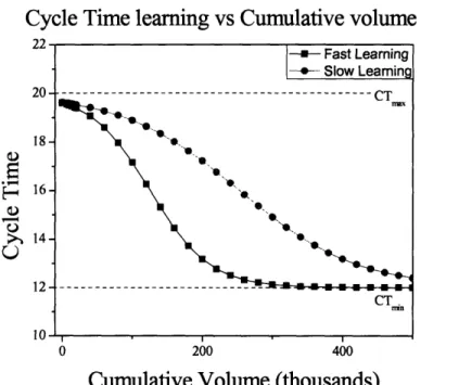
for the S curves... 54

3.2.2.3 Illustration of using normalized S curve to determine learning parameters (cycle time) versus cumulative volume ... ... 56

4. Case of Tube hydroforming ... 59

4.1 Dynamic tube hydroforming model... 59

4.1.1 Tube hydroforming model ... 59

4.1.2 Incorporating S curve learning model into hydroforming model ... 60

4.1.2.1 Determination of S curves from the data ... 60

4.2 Identifying critical learning levers ... ... 65

4.2.1 Case study for identifying critical learning levers ... 68

5. Process Variable Learning Cost Model Taxonomy... ... 71

5.1 Taxonom y Categories ... ... 73

5.1.1 Determination of Taxonomy Dimensions... ... 73

5.1.2 Taxonomy Dimensions Used in This Study ... 74

5.1.3 Definitions of Taxonomy Categories... .... ... 74

5.1.3.1 Capital (vs. Labor) Intensity ... 76

5.1.3.2 Material Intensity ... 77

5.1.3.4 Scope of improvement in Cycle Time, Down Time and Reject Rate... 79

5.2 Analysis of the Taxonomic Scenarios... ... 80

5.2.1 Description of the Baseline Process Model ... 80

5.2.1.1 Calculating Capital and Labor Intensive Scenario Inputs... 81

5.2.2 Impact of Learning on Different Types of Processes ... 82

5.2.2.1 Scenario 1: High Learning Rate & Scope for All Variables... 83

5.2.2.2 Scenario 1': High Learning Rate & Scope for All Variables with Growing Annual Production Volume ... 88

5.2.2.3 Scenarios 2, 3 & 4: High Learning Rate & Scope for One Variable Only93 5.3 Using the Taxonomy Model to Calculate Cost Evolution ... 97

5.4 Comparing the Taxonomy and Detailed Cost Modeling Approach Using the Tubular H ydroform ing Case ... 98

6. C onclusion ... 101 7. Future W ork ... 104 R eference ... 107 A ppendix A ... ... ... 112 Appendix B ... 115 Appendix C ... 118

List of Figures

Figure 1: Wright's learning curve... 21

Figure 2: Cumulative average S-shaped learning curve proposed by Carr (1946)... 22

Figure 3: Learning curve with steady state phase (saturation) (Baloff 1971)... 24

Figure 4: Comparison of learning curve models (Badiru 1992) ... 27

Figure 5: Effect of learning rate on cost evolution of fuel cells (Tsuchiya 2002)... . 31

Figure 6: Illustration of Process Based Cost Modeling ... 35

Figure 7: Available operation time based on a 24 hour day clock (Fuchs 2006) ... 37

Figure 9: The comparison in learning trends shown by s curves and log linear curves ... 49

Figure 10: Learning curve in terms of dimensionless learning parameter y*... 51

Figure 11: Normalized learning curve (normalized with respect to learning parameter and cum ulative volum e) ... ... 52

Figure 12: Derivation of alpha and beta for fast learning s-curve ... 55

Figure 13 : Evolution of cycle time with volume for fast and slow learning rates ... 58

Figure 14: Down time vs. cumulative volume... ... 62

Figure 15: Cycle time vs. cumulative volume ... ... 63

Figure 16: Total cost for tube hydroforming as a function of volume... 64

Figure 17: Cost evolution for tube hydroforming on elemental cost basis... 65

Figure 18: Effect of learning for different process variables on cost evolution ... 68

Figure 19: Cost saving per part pertaining to improvements in different parameters ... 69

Figure 20: Cumulative cost saving for cycle time and down time learning ... 70

Figure 21 : Illustration of the framework based on the classification levers ... 75

Figure 22 : Cost per part vs. cumulative volume for no growth scenario for material and Capital intensive (MC), Material and Labor intensive (ML), Non-material and Capital intensive (NMC) and Non-material and Labor intensive (NML) industries. ... 84

Figure 23 : Cost per part break down with respect to labor, material, equipment and tool for (a) material and Capital intensive (MC); (b) Material and Labor intensive (ML); (c) Non-material and Capital intensive (NMC) and (d) Non-material and Labor intensive (N M L) industries ... 86

Figure 24: Effect of learning on labor, equipment, material and tool (no growth scenario)

...,,,... 87 Figure 25: Cost per part vs. cumulative volume for 20% growth scenario for material and Capital intensive (MC), Material and Labor intensive (ML), Non-material and Capital intensive (NMC) and Non-material and Labor intensive (NML) industries. ... 89 Figure 26: Cost per part break down with respect to labor, material, equipment and tool for (a) material and Capital intensive (MC); (b) Material and Labor intensive (ML); (c) Non-material and Capital intensive (NMC) and (d) Non-material and Labor intensive (N M L) industries ... 90 Figure 27: Effect of learning on labor, equipment, material and tool for growth scenario

... 9 1

Figure 28 : Cost evolution for Scenarios 2, 3 and 4 for material, capital intensive industry

... 9 4

Figure 29: Cost evolution for Scenarios 2, 3 and 4 for material, labor intensive industry95 Figure 30 : Cost evolution for Scenarios 2, 3 and 4 for Non-material, capital intensive industry ... 96 Figure 31: Cost evolution for Scenarios 2, 3 and 4 for non-material, labor intensive industry ... 96 Figure 32 : Comparison of cost evolution between hydroforming data and taxonomic scenario ... 100 Figure 33: Evolution of cycle time, down time and reject with time for tube hydroforming analysis (generated using the S-curves) ... 114 Figure 34: Cost per part break down with respect to labor, material, equipment and tool for (a) material and Capital intensive (MC); (b) Material and Labor intensive (ML); (c) Non-material and Capital intensive (NMC) and (d) Non-material and Labor intensive (NML) industries for scenario 2 (only cycle time learning present) ... 118 Figure 35: Cost per part break down with respect to labor, material, equipment and tool for (a) material and Capital intensive (MC); (b) Material and Labor intensive (ML); (c) Non-material and Capital intensive (NMC) and (d) Non-material and Labor intensive (NML) industries for scenario 3 (only reject learning present) ... 119

Figure 36: Cost per part break down with respect to labor, material, equipment and tool for (a) material and Capital intensive (MC); (b) Material and Labor intensive (ML); (c) Non-material and Capital intensive (NMC) and (d) Non-material and Labor intensive

List of Tables

Table 1 : Effect of scope on cost evolution... 67

Table 2: Initial and final values for the process parameter... ... 68 Table 3: Model inputs for different industry scenarios... ... 82 Table 4 : Scenarios based on the scope levers (rate of learning is high in all these

scenarios) ... 83 Table 5: Scenario possible for given number of learning levers ... 105

1. Introduction

1.1 Study of cost evolution with time

In the 2 0th century, industries of every form have had to deal with a number of

externalities which drove a nearly continuous change in technology. There have been significant changes in policies and consumer demand over the last three decades that have resulted in advances in material and manufacturing process. The policies pertaining to the environment have become more stringent and consumer demand has shifted to more personalized products. In response to these changes, industries were forced to adopt newer and more effective technology, or else they feared the chances of being left behind. In this context, firm decision-makers repeatedly face critical questions of what technologies to select and when to apply them. Similarly there might be issues with making production strategy decision, for example, will it be more effective to produce a part in house or to outsource its production. Making a decision based on present time cost data will lead to misleading results, similarly making a decision on some speculated future ball park number might be wrong. For savvy decision-makers a key element of answering these questions depends upon their understanding or projection of how new technologies would evolve and develop over time. The focus of this thesis is to present an analytical framework that allows decision makers to better incorporate information about technology evolution into their technology decisions.

For an outside observer, it is pretty simple to point out that whenever a new product or a new technology is launched its initial cost of manufacturing is usually quite high, but with the passage of time the cost of production goes down. The driving force behind this

observation has been the focus of a various researchers over the past seven decades. This began with a study by Wright (Conway and Schultz 1959) who observed a simple phenomenon: the man hours involved in airframe manufacturing decreased as the cumulative number of frames increased. Wright concluded that the decrease in man hours and its resulting decrease in cost were due to experience gained by the workers as more parts were produced. This led Wright to propound the now-famous learning curve concept in which a process improves by some percent as the volume of production is doubled. Inspired by this work, researchers began to apply the knowledge of learning curves to a variety of different industries in an attempt to decipher their learning trends and predict their future costs.

The evolution of cost for different industries has been shown to be very different from each other and varies with product, technology, and capital investment. Grubber (1992) studied this phenomenon for various semiconductor memory chips. According to his observations, the cost curves for EPROMs are mainly determined by the cumulative output, confirming the learning curve hypothesis. However, for DRAMs, economies of scale were more important than learning. Baloff (1967) made similar observations in steel startups. Even though the processes involved in steel production are very similar across companies, they exhibit significantly different learning parameters. Baloff also compared the learning parameters for 17 different startup firms and demonstrated how the learning pattern varied with industry. These differences present a new challenge for decision makers looking to estimate learning patterns and cost trends for different types of industries.

One of the major motivating factors for the study of learning curves has been to understand the cost evolution trends of the past and try to use them to guide decisions about the future. The use of learning curve may provide a mean for better estimate in this direction.

Researchers in the past have used the concept of a learning curve as a tool for formulating future strategies (Amit 1986). Much of the work has focused on relating the reduction in average cost to the cumulative output of the process (Alchian 1963; Baloff 1971; Stobaugh and Townsend 1975). This work has largely relied on the use of regression analysis of historical price data without addressing the mechanisms by which costs decrease and the specific driving forces behind cost reduction. There are some cases where it would be interesting to know where costs were going even if one can't influence it, although admittedly, it is obviously better to know how to influence it as well. But there's another point. Predicting future costs for new products or processes through the use of historical data is only justifiable if the cost drivers for these products are structurally similar to those of the existing product. Consequently, understanding the mechanisms by which costs evolve is a necessary part of this type of analysis.

This thesis will look at the problem of cost evolution by breaking down the manufacturing process and studying both the major underlying cost drivers and the mechanisms by which learning within these drives cost change. In particular, this thesis will address how learning influences process variables such as cycle time, down time, reject rate and material cost and in turn, how these variables interact to yield cost reductions. This approach provides not only an understanding of how cost is expected to evolve with time but also understanding of the manner by which this occurs.. This will

not only help industry with future cost estimates, but will give guidelines as to how to best achieve these cost reductions in the most timely fashion.

1.2 Previous Work

The learning curve theory is based on the observation that the cost of an item depends on cumulative volume produced which is a function of the production rate and the time frame over which production has or will occur. This theory is usually attributed to J. P. Wright, who introduced a mathematical model (1.1) describing a learning curve in an article published in The Journal of Aeronautical Science titled "Factors Affecting the Cost of Airplane." (Wright 1936) Wright showed that the cumulative average direct labor input for an aircraft manufactured on a production line decreased in a predictable pattern. The decrease was related to the increased proficiency (i.e., learning) of the manufacturing laborers on the line as they performed the various repetitive tasks. The model described the learning as an exponential function which is as follows.

h =

aV

-b (1.1)

V = production count

h, = labor hour required for the V

th _unit

a = labor hour required for the first unit, hence a=h1

b = exponent of learning

The rate of progress is given by the complement of reduction that occurs with doubling of production volume. In the learning literature, a learning curve is referred to as an '80% learning curve' if the cost reduces by 20% every time the cumulative volume is doubled.

That is;

h2 = a(2V)-b = 0.8 _(1.2)

h, aV-b

h2v = 2-b = 0.8 b = 0.322 (1.3)

For an 80% learning curve the value of b will be 0.322

Arrow (1962), cited a Swedish iron plant (Hordal iron works) which had witnessed a 2% productivity increase in output per man hour even though there had been no new capital investment in past 15 years. He attributed the increase in productivity to the experience gained 'learning by doing' by the plant workers. The 'learning by doing' aspect of the learning curves was further expanded by Bahk etal (Bahk and Gort 1993), who tried to decompose it into organizational, capital and manual task learning.

The learning curve proposed by Wright had cumulative volume as the only factor responsible for a reduction in labor hours. Conway and Schultz (1959) pointed out that the method of manufacturing is also influenced by the rate of production and the estimated duration of production at this rate which gives the cumulative volume. Similarly Carrington (1989) pointed out that total cost is a function of cumulative output as well as the firms rate of output. Carrington also pointed out that marginal cost must be rising in general for the firm to be a part of competitive industry but most econometric studies of cost functions (1.1) fail to substantiate this implication.

Boston Consulting Group (Henderson 1972) added a new dimension to the concept of learning curves in late 1960s when it demonstrated that learning curves not only encompass labor cost but also administrative, capital and marketing costs. These analyses have included studies of refrigerators in Britain, polystyrene molding in USA, production of integrated circuits, direct cost of long distance telephone calls in the United States, and motorcycle production in Japan and Britain. This led to further recognition of the wide applicability of learning curves.

Hartley (1965; Hartley 1969) applied the concept of learning in the aircraft industry. Similarly, Baloff showed how the concept could be applied to labor intensive industries like automobile assemblies, apparel manufacturing and production of large musical instruments (Baloff 1971). Dudley (1972) soon followed and showed that a similar trend existed in the metal products industry. Zimmerman (1982) and Tan et al. (Tan and Elias 2000) showed that learning curves could even be used in the construction industry. Lieberman (1984) and Sinclair et al (Sinclair, Klepper et al. 2000) showed how the learning concept could be extended to chemical manufacturing plants. Other studies in this direction have been made by Preston et al. (Preston and Keachie 1964) for radar equipments, Grubber (1992), Chung (2001), Grochowski et al (Grochowski, Hoyt et al. 1996), Dick (1991) and Hatch (Hatch and Mowery 1998) for semiconductors, Sultan (1974) for steam turbine generators, Jarmin (1994) for the rayon industry, Argote et al. (Argote and Epple 1990) for manufacturing, and Tsuchiya (2002) to predict the cost of fuel cells.

Stobaugh et al. (Stobaugh and Townsend 1975) studied the price change for eighty-two petrochemical products over a time period of one, three, five and seven years as a

function of number of competitors, product standardization, experience and static scale economies. They concluded that by the time a petrochemical has three or more competitors, experience has a much larger effect on price than the other three factors.

Liebermann (1984) also observed similar trends after he analyzed the three year price change for thirty-seven chemical products. He examined several other candidate explanatory variables of learning such as time, cumulated industry output, cumulative industry capacity, annual rate of industry output, average scale of plant, rate of new plant investment, rate of new market entry and level of capacity utilization. After analyzing all of the parameters he concluded that the cumulative industry output is the single best proxy for learning.

In most real-world cases, experience curves reflect the convolved effects of learning, technological advances, and economies of scale. Generally, it is difficult to distinguish between the contributions of economies of scale and learning because both tend to occur simultaneously. Learning generally results in better utilization of resources which leads to higher and more efficient production. Efficient production means higher potential volumes which if realized result in economies of scale. Few studies have tried to decouple the effects of learning and economies of scale. In one study, Hollander (1965) analyzed the sources of efficiency increase at a DuPont rayon plant and concluded that only 10-15% of the efficiency gains were due to scale effects, whereas the rest were accounted for by technology and learning. Hollander found that a large part of the cost reduction from technology improvement could be attributed to a series of minor technical changes. This could be justified to some extent as learning by observation because generally, over time, engineers in a production facility "learn" to tweak the machinery in

a way to give maximum production efficiency. Sinclair (Sinclair, Klepper et al. 2000) also looked at cost reduction in specialty chemical divisions and observed that technology triggered cost reductions were largely the result of small technological changes in production and manufacturing based on R&D and related activities.

Significant work has also gone into using learning curves to develop firm operational strategies. Spence (1981) developed a model of competitive interaction and industry evolution in the presence of a learning curve. He concluded that, under certain conditions, if a firm can lower its future costs by increasing current production, then the firm should produce parts even if this is not the short term profit maximizing strategy. By doing so, the firm achieves higher profits in the long run by moving further down the learning curve faster than its competitors. The learning curve also creates entry barriers and protection from competition by conferring cost advantages on early entrants and those who achieve large market shares (Spence 1981; Porter 1984; Lieberman 1989). Spence's

analysis also showed that the largest barriers to entry occur when there are moderate rates of learning rather than when there is either very slow or very fast learning.

The form of the learning curve has been debated by many researchers and practitioners. However, Wright's learning curve is, by far, the most widely used and accepted (Henderson 1972; Lloyd 1979; Day and Montgomery 1983; Lieberman 1987). The method that is commonly used by most of researchers is to look at the industry data and try to find a relationship between various parameters. This regression analysis of the industry data gives a relationship between various parameters which can be extrapolated to predict future cost trends. All these analyses result in different patterns for a set of industries without indicating how to influence the trend.

1.3 Learning Curves and Concept

A variety of functional forms have been used for learning curves. The choice of a functional form depends on the way costs decline over time. Some suggest that doubling the cumulative volume results in decrease of cost while others argue that this decline in cost cannot be sustained forever and should reach some saturation.

The most common form of experience curve is given by

C, = Con - (Wright's Learning Curve)

This can be written as In C, = In CO- A In n

(1.4)

(1.5)

This equation implies a constant decline in unit cost each time n units are produced (Figure 1)

2 3 5 7 10 20 30 50 70 100

Cumulative units (hundreds)

Figure 1: Wright's learning curve

I I 1 1 11_11 I . I I 1 1_1_

Wright's model describes the learning of a new product 'start-up phase'. It is based on the idea that the decreases in labor hours can be sustained forever. However, in practice, the decrease cannot continue indefinitely and eventually saturation would be expected to take place. As a result of this saturation production reaches a kind of steady state where the direct labor hours remain constant.

C

a06

1

6

4

Cumulative unit number

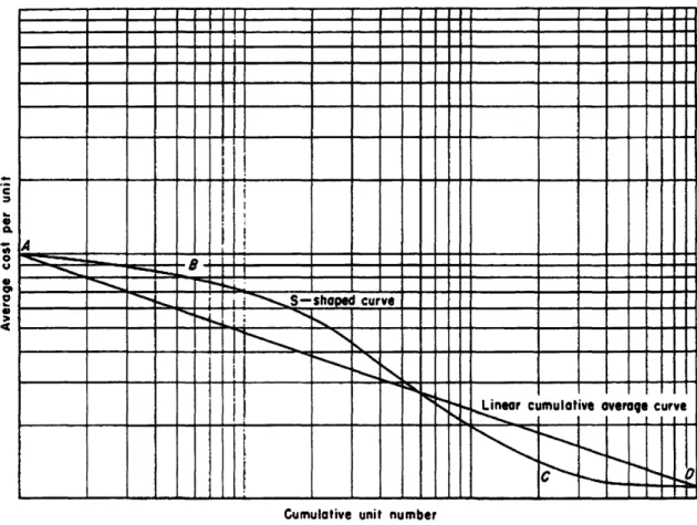
Figure 2: Cumulative average S-shaped learning curve proposed by Carr (1946)

Carr (1946) argued that shape of the learning curve should be S in nature rather than a straight line. He explains the concavity in this curve (Figure 2) by first assuming that each worker in all the production crews hired for a particular job produces along an 80 percent curve. However, the crews are not all hired at the beginning of the program but are hired one at a time during the acceleration period. Hence the crew works at different

points of their individual linear cumulative average progress curves at the same point of time. This would lead to concavity in the learning curve. While Carr does not explicitly state the saturation effect in his approach, his proposed learning curve incorporates the essence of saturation at the later stages of production.

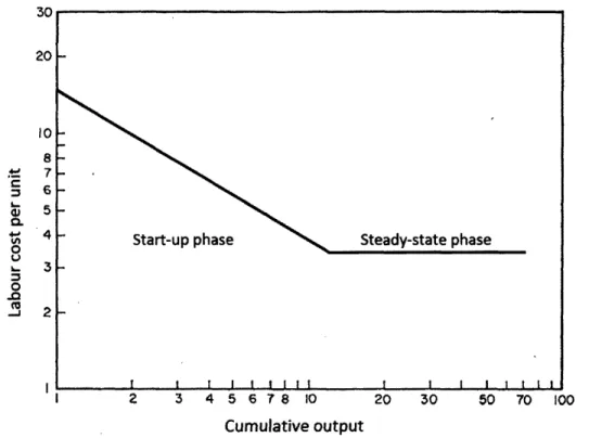
Baloff studied this plateauing phenomenon (Figure 3) and found it to be extensively present in machine intensive manufacturing. He studied twenty eight separate cases of new product and new process startups that occurred in four different industries and observed plateauing in twenty of the cases. In a subsequent study, while analyzing data for musical instrument manufacturing and automobile assembly firms (both of which were labor intensive in nature), Baloff (1971) found that some sets of firms within these industries reached steady state in the long run. However, the time to reach the steady state was higher for labor intensive industries. Yelle (1979) postulated that the reason for this observation could be smaller progress ratio for machine intensive learning or management's unwillingness to invest more.

Another likely reason the saturation effect is often not included in the learning curve is that the life cycle of the product might be short, and thus the production may never reach the steady state during the time of observation. Past analyses have often focused on product rather than manufacturing processes used in the industry. Long term study of manufacturing process data would be more likely to show the saturation effect.

However, Wright's approach can be easily modified to include the saturation effect as shown in Figure 3.

30 20 10 8 . 7

5

4% 4 L 3 0 -o -J 2 I 2 3 4 5 6 78 10 20 30 50 70 100 Cumulative output

Figure 3: Learning curve with steady state phase (saturation) (Baloff 1971)

Other notable learning models include

1. The Stanford-B model

This model derives its name from Stanford Research Institute, where an early study commissioned by US defense department led to this model. This model was found to be more representative of World War II data compared to log linear learning curves. The model is represented as:

Yx = C,(x + B)b (1.6)

Yx :direct cost of producing xth unit C1 :direct cost of first unit

B :constant (1<B<10), equivalent unots of previous experience at start of a process It is noted that when B=O, then this model reduces to the log normal model

2. DeJong's learning formula

This model uses a power functions which incorporates parameters for the proportion of manual activity in a task. DeJong's formula introduces an incompressible factor, M, into the log linear model to account for the man-machine ratio. The model can be expressed as follows:

MC = CM + (1 - M)x-b] (1.7)

MC, = Marginal cost for producing x'h unit M = Incompressibility factor (constant)

When M=O the model reduce to the log-linear model, which implies a complete manual operation. If M=1, then unit cost becomes equal to C1 which suggest that

there is no cost improvement possible in machine controlled operations.

3. Levy's adaptation function

Levy recognized that the log linear model could not account for the leveling off of production rate and the factors that might influence learning. In light of this observation he proposed the following model:

MCX = 1 1 k

(1.8)

8:production unit for the first unit

k : constant used to flatten the learning curve for large values of x

The flattening constant k causes the curve to reach a plateau instead of continuing to decrease or turning in the upwards direction.

4. Knecht's upturn model

Knecht observed the divergence of actual cost from those predicted by the learning curve theory at higher production volumes. He modified the basic functional form of the learning curve to avoid zero limit unit costs at large volumes. He altered the expression for curve to allow an upturn in the learning curve at larger values of cumulative production volume. The form suggested by him is as follows:

Cx = CIxbe" (1.9)

c = constant

5. Glover's Learning Formula

This model is based on a bottom up approach which uses individual worker learning results as the basis for plant wide learning curve standards. The functional form of the model is expressed as:

Xy]

+a = C[ x (1.10)

i=1 i=1

y, : elapsed time of cumulative quantity

x_i : cumulative quantity or elapsed time

a : commencement factor n : index of curve (usually l+b) m: model parameter

6. Pegel's exponential function

Pagels learning curve has an exponential functional form and it is represented as:

a, ,, a :parameters based on emperical data analysis

7. Multipicative power model (Cobb-Douglas)

The multiplicative model can be used to represent various factors which might influence the cost of production. The independent variables can vary from to include both tangible and intangible parameters which might affect future costs.

C = k xx x x. ... * * x, (1.12) C: estimated cost k: model constant x,: i't independent variable b,: exponent of ih variable : error term

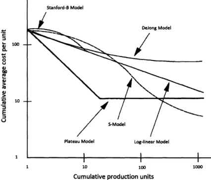
These formulas have differed in their functional forms and can be seen below (Figure 4).

CU 100 CL In 0 U a) m 4.0 +J 10 E U I 1 10 inn

Cumulative production units

1.4 Application of learning to industry

Learning curves have been extensively used in industry in various forms and with different perspectives. It has undergone a wide transformation in its understanding and application since it was first coined by Wright in 1936. Initially, researchers had used learning curves as a tool to predict how the labor hours for manufacturing would evolve over time. With time, the scale of measurement changed from labor per hour to labor cost per unit and finally to cost per unit produced.

On similar lines the various factors used to justify the learning trends also increased and became more comprehensive in nature. Wright believed that learning happened due to repetition of task alone, but later researchers have included many other factors to justify the learning curves.

Some of the learning processes can be listed as follows (Badiru 1992; Malerba 1992; Goldberg and Touw 2003)

1. Learning by doing: This form of learning is internal to a company and depends upon the production activity.

2. Learning by using: This form of learning is also internal to a company and is related to the use of resources, machinery and other inputs

3. Learning from advances in science and technology a. Basic Science

c. Engineering

This form of learning can be internal or external to a company and depends upon development or adoption of new technology.

4. Learning from inter-industry spill over: Acquiring technical knowledge developed by the competitor.

5. Learning by interacting: This form of learning is external to a company and depends upon the level of interaction with upstream or downstream sources of knowledge within or outside the firm. The outside knowledge can come from the suppliers or with knowledge sharing with other firms in the industry.

6. Learning by searching - Internal to a firm and related to activities aimed at generating new knowledge base (like R&D).

Similarly, other researchers have also tried to incorporate the effect of management decisions, industry structure, competition, etc. into the learning curve. This has undoubtedly shown the power of learning curves and their importance to the industry, but has made their application very cumbersome and often quite difficult. In the literature learning has been shown to be pervasive. However, as the next section will detail, there are limits to how learning curves can be used to guide technology selection decisions.

2. Current approach and proposed methodology

2.1 Shortcomings of the current approaches

Until recently, most of the research done in this field has taken a top down approach to understanding cost reductions over time. Researchers have taken an aggregate outlook towards this problem. The general approach has been to regress data of cost per unit against cumulative volume (Tsuchiya 2002) and to understand the patterns followed by different industries and products. Figure 5 shows the work done by Tsuchiya et al. In this work, the cost of fuel cells has been calculated over time for nine different scenarios depending upon the power density of fuel cell (L, M and H for Low, Medium and High) and cost reduction speed for material(A, B and C for fast, medium and slow) used to make the fuel cell. It has been assumed that cost would be reduced by some fixed percentage for different scenarios, based on some speculations. Using different assumed rates of learning, the cost of fuel cells has been calculated over a period of time.

This study is based on an underlying assumption that the cost reductions observed for existing technologies can be applied to future products/technologies, such as fuel cells. Such an assumption must be made with great caution and only with deep understanding in the related field of technology. Otherwise such a speculation might make the learning curve look like self fulfilling prophecies.

Secondly, it can be difficult to explain cost reduction for a technology based on just a single variable, i.e. cumulative production by applying some pre determined learning rate to it.

Learning effect of nine scenario

10,000

1,000

1O0

10

.1 0 (, (A u :3 !1

on cost evolution of fuel cells (Tsuchiya 2002)'

Finally, this approach also neglected the effect of changes in technology which gave an impression that this technique is technology blind.

While learning curves are valuable for estimating future costs, an additional significant contribution should be to help managers and engineers make decisions. The decision should be based on a technical understanding of the learning effects on production, not just the resulting cost reductions.

The current method of analysis, based on regression just tells the managers to produce some quantity of parts before their cost can be expected to go down to a certain level. It

i In the figure, H, M and L stand for high, medium and low power density. A, B and C represent scenario of fast, medium and slow cost reduction for the cost of material used.

o o

o-o o 0

C54 El n rJ

5: Effect of learning rate Figure

LC

-- M C

HC

SLB

--- M B -.- H B

-+- LA

---- M A

---HA

___ i to 00 0ý C%1 I~ to 00 C) C> O T- T- T,- T-- C O O O O O O C> C> CC CD C C) C. CN4 C14 C'%J C-4 04 C.J C C.J 'i %

does not probe deeper to understand the reasons that actually caused the cost of production to go down. If the managers and engineers could be given a perspective about the factors actually affecting the cost of production, and their contribution in bringing down the cost, they would be in a better position to decide future strategies for production.

For example, suppose a regression analysis of a data set gives a result that a product follows an 80% learning curve (Wright 1936). This result provides a variety of information. First and foremost, it indicates that the cost of production goes down by 20% each time the production volume is doubled. Second, it indicates the cumulative production volume needed to achieve a given cost target. However, an engineering perspective about the production improvements that will lead to these cost reductions is missing. There is no way to know if the same cost reductions could be achieved through specific technical advances instead of increased production. A method that decomposes the cost analysis into smaller parts would allow the engineer to pinpoint the factors that influence cost and thus provide other means to achieve cost savings besides increased production.

2.2 Proposed methodology: A process based cost modeling approach

To analyze the affect of learning curves on production it is essential to break down a production process into its constituent sub-processes and understand how learning applies to each of these sub processes. It is much simpler to understand the learning process at a sub-process level compared to aggregate level. Furthermore, it gives engineers and managers insight into the causation factors. The break down of a specific production process and its analysis is achieved by using a technique developed at MIT's Materials

Systems Laboratory entitled Process Based Cost Modeling.

Process Based Cost Modeling (PBCM) (also know as Technical Cost Modeling) is a powerful analytical tool that integrates elemental costs derived from technical and operational drivers to estimate the total cost of production (Kirchain and Field 2001). PBCMs allow one to predict manufacturing costs for new designs, using well characterized processes, by relying on engineering fundamentals of the manufacturing process rather than historic data.

A specific manufacturing process can be looked at with respect to some factors such as reject rate, down time, cycle time, equipment cost, tool cost, and material cost; and the concept of learning curve can be individually be applied to each of these factors. These factors can then be passed into the PBCM to get the cost per part being produced. (2.1)

This decomposition of cost into these tangible factors allows for insight into causation talked about earlier. However to use the process variables like (cycle time, down time and reject) one still needs to make separate predictions. In this case uncertainty of forecasting still exists, but it is focused around tangible technology and operational aspects. This gives the engineers a scope to apply their subject matter expertise to build confidence around the predictions made.

3. Structured cost modeling approach

3.1 Process based cost modeling

Process based cost modeling (PBCM) is a method for analyzing the cost of manufacturing technologies by capturing the key engineering and process characteristics which relate to the total production cost of a component. PBCM is an improvement over the previous cost estimation techniques which relied on rules of thumb, past experience and accounting practices.

0

'too C1

Il ·

Il

IEm

.cr

_CL

D!E

Er

00

Onrtain I

tVo go,

r

actor

Conditions

_Prices

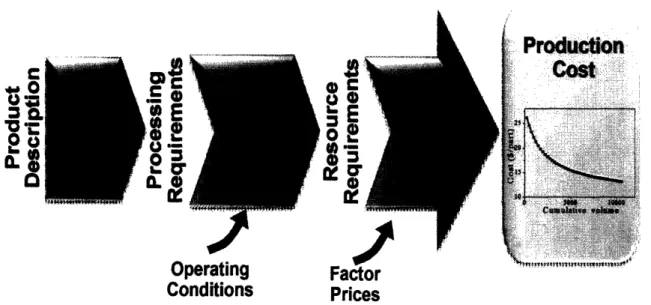
Figure 6: Illustration of Process Based Cost Modeling

For practical purposes, the PBCM can be broken down into three sub-models as shown above (Figure 6). The first one describes the processes needed to produce the part. The next model considers the operations of the manufacturing facility. The final model

3.1.1 Process Model

The process model is built on strong pillars of science and technology. It uses the principles of engineering and science to calculate the processing parameters (Figure 6). The process model requires inputs for the size, shape and material of the final product. Depending upon the technology and material inputs, the process model calculates the total cycle time for the process. The model also gives output for the equipment capacity (for example, size and tonnage in case of press) and tools which might be required to carry out the process. Since the process model is governed by the engineering principles, it also addresses the constraints on cycle time and reject. For example, for a deformation process there is a limit on maximum strain rate at which a defect free part can be produced. The cycle time for such a process cannot be lower than that calculated by this maximum strain rate. Similarly for semiconductor industry there is a minimum number of reject that will be produced depending upon the thermodynamics of the processing technique. In no situation the reject rate can be lower than this value. The processing requirements augmented with the operating conditions including the shifts schedule, working hours, desired annual production volume, etc., are passed into the operations model.

3.1.2 Operating Model

The next part of the PBCM is the operating model, which determines the time required to meet a given target production volume (required operating time). Once the time is calculated, number of parallel lines can be determined based on the total time available (uptime) in a year and therefore the scale of the production facility. This information is

then used to calculate the total amount of equipment, labor and other resources needed to achieve the desired product output.

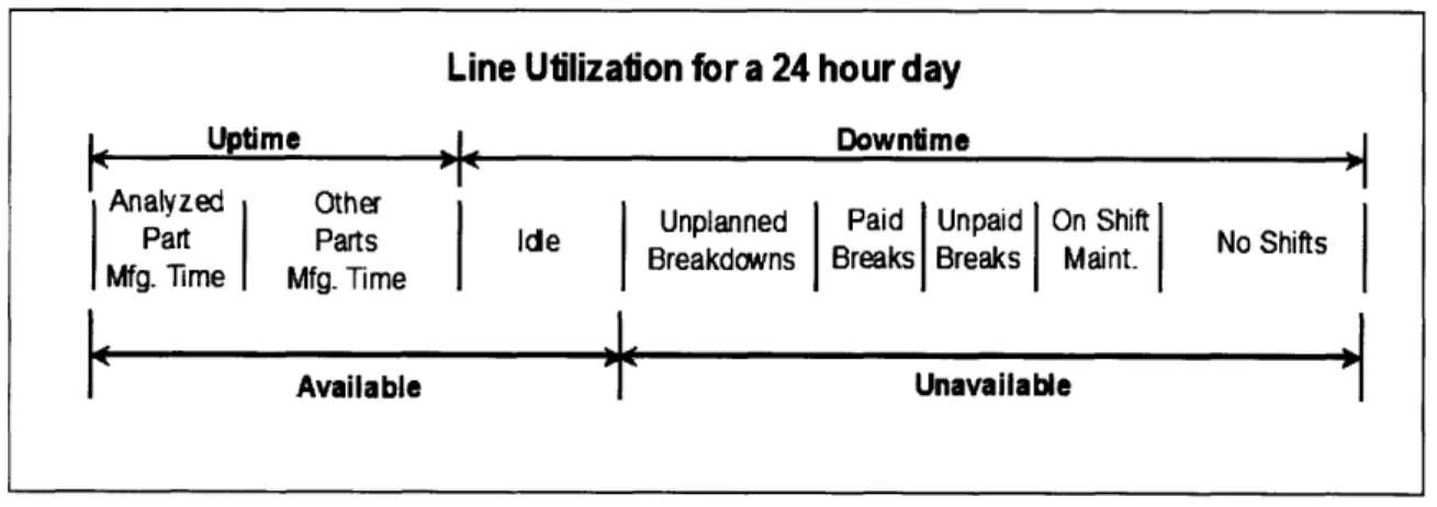
a. Annual Available Operating Time and Uptime

The calculation of annual available operating time involves the integration of several available metrics. The line utilization for a day can be divided primarily into available and unavailable time. The available time includes the time when the plant is manufacturing and also the idle time when the plant is staffed and running but is not producing due to a lack in of demand. The unavailable time includes unplanned breakdown, worker breaks, maintenance time and the time when the facility is not operating (Figure 7).

Figure 7: Available operation time based on a 24 hour day clock (Fuchs 2006)

The available line time can be calculated as:

AT = DPY.(24- NS -UB- PB -UD) (3.1)

Line Utilization for a 24 hour day

Uptime I, Downtime

rAnalyz Other Unplanned _{Paid Unpaid On Shift}

Part

Parts

idle

_{No Shifts}

Part i Mide Parts Breakdowns Breaks I Breaks Maint.

Mfg. Time Mfg. Time

AT: Available line time DPY: Days per year NS :No Shift

UB: Unplanned breakdown PB :Paid break

UD: Unpaid break

Finally, the uptime for the line can be calculated as the time when the line is running and actually producing the desired parts.

UT = AT- Idle

b. Annual Required Operating Time

Annual required operating time is the total time required to produce the target number of parts and is defined as the product of cycle time and number of parts required annually (3.2). Since target volume of production for a given year is known, equation (3.3) can be used to determine the actual number of parts which is required to be produced based on the reject rate.

t = CT * n (3.2)

n

ni-1 (3.3)

1- reject,_₁

CT = Cycle time for process i

n; = number of parts at the ith sub process

rejecti = reject rate in fraction for the ith sub process

Annual available operating time tells us the amount of time a single line would be running in a year. This can be used to calculate the number of lines that would be required to attain the target production volume. The number of lines can be calculated by dividing the annual required operating time by the uptime (3.4)

nl = (3.4)

UT

nl = Number of parallel lines

Annual paid time equation (3.5) is used to calculate the time for which the labors are paid. It is defined separately from annual available time to account for paid breaks and unplanned downtime for which labors are paid.

APT = (24 - NS

-

UB).nl

(3.5)

3.1.3 Financial Model

The final part of the PBCM is the finance model which works in conjugation with rest of the model to eventually calculate the unit cost of the product. The role of the financial model is to apply unit prices to the levels of resources consumed as determined by the operations model and to correctly allocate the costs over time and across products. The cost element can be broken down into material, labor, energy, building, equipment, tool and overhead cost. Each of these cost are calculated separately using the information from the previous models to give the total cost (Fuchs 2006)

Ctotai = Cmaterial + Clabor + Cenergy + Cbuilding + Cequipment + Cools + Coverhead (3.6)

The cost of material, labor and energy are considered to be variable costs and therefore can be directly applied to the cost of the product. However, some allowance is needed to

account for the variable costs associated with downtime, rejected parts, etc. The financial model is also used to sum the individual cost elements to determine a fully accounted unit cost of production(3.6).

Material cost is the product of number of parts produced, weight of the product and the price per unit mass of the product. The scrap which is produced is sold as at scrap rate

and is credited from the material cost

Cmateria = ni .W.P - (ni - no ).W.Pcrap (3.7)

n, : Total number of parts produced to meet the demand n, - no : Number of scrap

W: Weight of product

P: Price of material per unit mass P, cra :Price of scrap per unit mass

Labor cost can be specified in three separate classifications - technician, skilled and unskilled labor. The annual cost can be calculated as the product of annual paid time, wage rate and fraction of line for which the production was carried out.

Clabor = XAPT·.Pi. (3.8)

AT

j: technician, skilled, unskilled labor

APTi :Annual paid time P : Wage rate

S:Fraction of line

Energy cost can be calculated in many different ways. Generally the energy cost can be calculated based on specified energy consumption rate for each machine. The energy cost is given as a product of annual required line time and the energy consumption rate for the equipment (3.9).

But some time the energy consumption can be tackled in a more comprehensive manner by using energy balance. This is generally used for process involving heating and the energy cost might be calculated on the basis of the thermal content supplied to the material and the thermal losses involved in maintaining the temperature for some fixed amount of time (3.10).

Cenery t.Ei

(3.9)

E, :Energy consumption rate for equipment i

Cener, = Energy absorbed by material + Rate of heat loss.Time (3.10)

Building, tool and equipment are considered to be capital investment. The capital investment is treated as fixed cost that must be spread over years of production. The financial model amortizes these investments over their useful lives to determine a series of equal annual payments equivalent to the initial investment. Time value of money is also factored into this calculation to ensure that the full costs of these investments are taken into account in the unit cost or production.

The opportunity cost of associated with capital investment is calculated using standard capital recovery factor (de Neufville 1990).

CRF. = r( + r) (3.11) 1

(l+r)"-l

CRFj : Capital recovery factor

j: Building, Equipment, Tool

r: Interest rate n :Number of years

The annual amortized cost for building, equipment and tool is the investment times the capital recovery factor equation(3.12). This is the amount of money which needs to be paid annually for using the resources.

ACj = CRFj. EI (3.12)

ACi :Annual cost for

j

CRFj :Capital recovery factor for j EIj : Capital investment made in j

The production cost obtained from process based cost model can be analyzed in different ways. Fixed costs versus variable costs can be examined, or these costs can be further broken down into the contribution to cost attributed to capital, labor, material, energy etc. Costs can also be explored by process step and each of the previous cost elements can be examined by process step as well. This type of model also provides a means to run sensitivity analysis with respect to various parameters which gives a more complete picture about how different parameters might affect the final price.

Such a detailed level of sensitivity analysis based on process variables is possible because the models are constructed to derive cost from the process level, and therefore do not use statistical methods to derive cost from the part description (Although statistical models are sometimes used within the process model to derive process conditions from part

descriptions). This makes this method a powerful tool to study the effect of various operational parameters on the cost of the part produced. The cost can be analyzed in different ways to understand how each of the parameters interacts with each other and the final cost. It can also be used to identify the primary drivers which affect the manufacturing cost.

o

F-h.r 0.--L_( C., (UIL L0n sluwaJ!nba

--eaJnoseN

0o 00 -o a0 C* O0 4) t-o 00

uondposec*

IfnpoJd

C4

3.2 Dynamic/Time Dependent Cost Model

In the previous section the power and usefulness of PBCM was demonstrated. However, these models provide cost estimates only at a fixed point in time. In this section, a method for expanding the use of PBCMs to address the question of cost evolution with time will be presented.

As discussed in the previous section, the process model portion of a PBCM is used to determine production parameters based on inputs related to final product. There are many process parameters which are included in a typical PBCM and each has their own impact in determining the final cost. Some of the common process parameters are shown in Figure 8, but this is not an exhaustive list and there might be others.

In a typical, static process based cost model, best case values for these variables are determined, often based on theoretical minimums. In practical situations, the values of these process parameters are often higher than those predicted by the model. This is due in part to an inability to ever achieve theoretical limits, but also reflects the fact that in some cases learning with respect to these variables is not complete, and therefore these variables have not yet reached their long term steady state values. Representing the values of the process parameters as a function of time or cumulative volume provides a good way to investigate the cost improvements possible over time. Compared to the top down approach of learning where total cost is treated as a function of time or cumulative volume, this method provides insight into the mechanisms that lead to cost reduction. Process engineers and technical specialists may be able to provide reasonable estimates

for improvements in production parameters thus leading to a better perspective on how to further improve the cost.

3.2.1 Using learning curves for process variables

As suggested in the previous section, the process variables can be expressed as a function of cumulative volume or time in the dynamic PBCM.

Process variables are likely to have several different phases of learning and therefore a learning curve approach which comprehends these concepts must be employed. These learning phases can generally be categorized as an initial transient phase, followed by a learning phase and finally a saturation phase.

The initial transient takes place just after the implementation of a new process. During this phase the improvements in the process parameters are slow. Initial transients are observed because just after implementation of a new process, it takes some time before line workers and engineers begin to understand the practical intricacies and details.

The second phase is the learning phase, which is characterized by major improvements in the process parameters. The improvements in this phase can be attributed to (Carrington

1989):

a. Job familiarization by the workmen, which results from repetition of manufacturing operations.

b. General improvements in tool coordination, shop organization, and engineering liaison

c. Development of more efficient sub assemblies, part-supply systems and tools.

After spending some time understanding the practical intricacies of the line, the line engineers are in a better position to apply their knowledge to improve the overall line performance.

The final phase is the saturation phase where improvements in the process parameters plateau. The saturation effect illustrates the fact that some of the parameters cannot be improved indefinitely and are constrained by laws of nature. Cycle time provides an excellent illustration of this concept. The cycle time will initially be high but may come down with time due to learning at an operational level. However, cycle time cannot go below a theoretical minimum value. This theoretical minimum could be related to physical limits based on scientific principles involved in the manufacturing process. For

example, limits to how quickly cooling can be accomplished will be based on principles of heat transfer. While there are often opportunities to reduce cooling times, eventually the laws of physics regarding heat transfer will limit any further reduction. Similarly, for processes involving chemical reactions, theoretical limits for reaction kinetics will result in a minimum possible cycle time. Once this minimum is achieved we can assume that the learning process is fully completed and there is no scope for further improvements with regard to this variable.

3.2.1.1 Selection of process variables

There are a number of process variable which can be represented as function to time or volume to showcase the effect of learning which can be used to determine the cost evolution. But the choice is based on the impact the variable is bound to make in the final

outcome. While there are many process parameters included in a typical PBCM, three variables in particular often have a strong impact on cost and are likely to improve with time as the process matures: cycle time, downtime and reject rate.

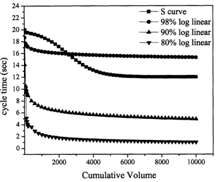
3.2.1.2 Trade off between S curves and log linear learning curves

The log linear learning curves (1.5) are based on the concept that learning takes place indefinitely over time and can be represented by a logarithmic function.

The positive aspect of using this curve is that only two parameters (initial value of process parameter and learning rate) need to be specified to obtain the learning curve. The major drawback of this type of curve is that it cannot account for the initial transient or the saturation phases appropriately. The log linear curve does attain some kind of saturation effect but since the saturation value cannot be specified, it generally occurs at values much lower than the theoretical limit (Figure 9).

The learning rate of log linear curves does not explicitly state whether the observed learning is fast or slow. It is very much dependent on the production volume of the product. For example, a learning rate of 95% might be a fast rate for a semiconductor company producing millions of chips annually, but it might be a slow learning rate for a turbine manufacturing company producing just thousands of units annually.

Even with these shortcomings, log linear curves have found widespread acceptance in the learning literature. The plausible reasons these issues are seldom raised in the learning literature could be that the life cycle of the product under observation is so short that the saturation level is never reached.

Z-4 22 20 18 16 8 14 12 S10 u 8

06

4 2 0 Cumulative Volume

Figure 9: The comparison in learning trends shown by s curves and log linear curves

The initial transient is generally not observed because the transient phase generally occurs in the R&D stages and the initial period of production, which is often not included in data collection. Data collection is generally started once the product is fully under production.

To overcome these problems, S shaped learning curves have been proposed. These curves provide more power and flexibility to capture the observations made with regard to the initial transient and saturation phases. The figure above (Figure 9) shows an S shaped learning curve. It can be seen from the shape of the curve that it can be used to represent the initial transient as well as the saturation effect, in a very effective manner. Compared to log linear curve it has a shortcoming in terms of number of parameters required to specify the curve. For S curves four parameters are required to be specified to

completely define the learning curve, as compared to log linear which requires just two. The tradeoff between the accuracy of curve representation and easy of collection data often determine the choice of the learning curves. It is left to the discretion of the user to make a decision between the two curves.

For the current study S curves were chosen over log linear curves to represent the learning behavior.

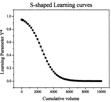
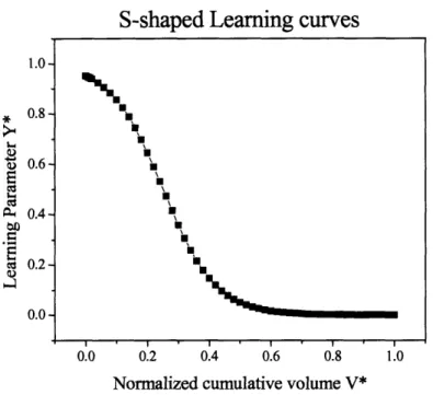
3.2.1.3 Benefits of using non dimension learning variables

Traditionally the S-curves (Carr 1946; Yelle 1979) were specified as process variable versus cumulative volume. The process variables learn and improve over a period of time. The improvement in the process variables can be expressed by using a non dimensional learning variable (y*) (3.13) which could be mapped to different process variables.

y PV-PVni"i (3.13)

PVn - PVmn

PV = process variable

The non dimensional learning variable (y*) varies between 0 and 1, (Figure 10) where 1 corresponds to its maximum value and 0 can correspond to its minimum value. The normalization increases the ease of application of learning curves to different process parameters.