Cycle-averaged models of cardiovascular dynamics

(1)

Cycle-Averaged Models of Cardiovascular

Dynamics

by

Jolie L. Chang

Submitted to the Department of Electrical Engineering and Computer

Science

in partial fulfillment of the requirements for the degree of

Master of Engineering in Electrical Engineering and Computer Science

at the

MASSACHUSETTS INSTITUTE OF TECHNOLOGY

June 2002

@

Jolie L. Chang, MMII. All rights reserved.

The author hereby grants to MIT permission to reproduce

Ud

distribute publicly paper and electronic copies of this thesis document

in whole or in part.

Author .

SSACHUSEMS ITTEUTE OF TECHNO.OGY

JUL

3 1 2002

LIBRARIES

BARKER

Department of Electrical Engineering and Computer Science

May 24, 2002

Certified by ...

George C. Verghese

Professor

.Thnis Supervisor

Accepted by ...

:.

.

...

Arthur C. Smith

Chairman, Department Committee on Graduate Students

MA

(2)

(3)

Cycle-Averaged Models of Cardiovascular Dynamics

by

Jolie L. Chang

Submitted to the Department of Electrical Engineering and Computer Science on May 24, 2002, in partial fulfillment of the

requirements for the degree of

Master of Engineering in Electrical Engineering and Computer Science

Abstract

A computational, circuit-based, hemodynamic model has been developed by Heldt

et al. in order to study the cardiovascular system's response to different situations and conditions. When studying the model's transient response over many heartbeat cycles, to perturbations such as lower body negative pressure or standing up, a cycle-averaged version of the model would seem to be sufficient. Such a model would suppress details of the periodic pulsing waveform of the heart beat, instead capturing just the cycle-to-cycle dynamics. Cycle-averaged circuit models are also expected to be more computationally efficient, and can be used to define and study control structures within the system that respond to averaged rather than instantaneous quantities. This thesis is focused on developing and studying such cycle-averaged models. In addition, we demonstrate that both pulsing and cycle-averaged models are very straightforward to implement in HSPICE, a commonly used circuit simulation package.

A simple circuit-based, one-ventricle, pulsing heart model is used throughout the

thesis. The pulsing action is captured in a time-varying capacitor, and the valve action through two diodes. This model was set up and studied in HSPICE. We derived from this pulsing model two cycle-averaged models, one involving three de-pendent sources, and the other with four dede-pendent sources. Both averaged models turned out to be linear and time invariant in their responses to initial conditions, and were therefore analytically very tractable when set up in state-space form. When simulated in HSPICE, both cycle-averaged models produced responses that followed, with reasonable accuracy, the actual cycle-averaged waveforms derived from the corre-sponding responses of the pulsing model. Due to the suppressed intra-cycle detail, the cycle-averaged models typically needed less than a tenth of the number of computed samples required by the pulsing model, and ran almost twenty times as fast.

The four-source averaged model was also used to represent the arterial barorecep-tor reflex, with feedback control of heartbeat period, zero-pressure filling volume, and peripheral resistance. Each of these controls, taken one at a time, was successful in counteracting changes in the average arterial pressure from its desired steady-state value. Future work can include: improving the accuracy of the averaged models still

(4)

further, by refining the assumptions made in their derivation; extending these models to the full hemodynamic model; and using these models for further study of dynamics, control, regulation, and identification.

Thesis Supervisor: George C. Verghese Title: Professor

(5)

Acknowledgments

First, I would like to thank my thesis advisor, Professor George Verghese, for all of his continued support and guidance throughout the last year. He was always available to help me with any problems I encountered along the way. His insight, experience, and enthusiasm made this project possible.

Thanks to Professor Roger Mark, my academic advisor and thesis co-supervisor, for his advice on my thesis, classes, and life at MIT and beyond.

Special thanks to Thomas Heldt for encouraging me and helping me to see how my project related to the bigger picture. He was always there to help provide insightful and useful suggestions.

Thanks to Siebel Systems for selecting me for the Siebel Scholars Program, which funded me for part of my M.Eng year.

I would like to thank all of the wonderful people I have met at MIT, which have

made my experiences interesting and lively. Specifically, thanks to Nori Yoshida for believing in me and for being there to support me for the last four years. He has helped me stay sane along every step of the way. Thanks to Alex Park for answering my endless questions about LaTEX, 6.003, thesis writing, and life in general. Thanks to Fong Keng for her constant and contagious smile during the past year. Thanks to the 6.003 Spring 2002 teaching staff for helping me through my last semester. I had a lot of fun teaching for the first time. Thanks to all of the lifelong friends I have made at MIT: Janice, Kathie, Wan-jen, Rich, Alan, Jack, Xuemin, Yi-fung, Eugene, Sanjay, Jessica, Cat, and Stephanie. And thanks to the countless people that have made the last five years memorable.

Finally, and most importantly, much thanks and love to Mom, Dad, and Anita for supporting me throughout all of my endeavors.

(6)

(7)

List of Figures

1-1

1-2

1-3

The circuit-based hemodynamic model. . . . . Time-varying capacitance waveform. . . . .

Response of the hemodynamic model to a stand test. . . . . 2-1 Simple RC circuit with time-varying capacitor. . . . . 2-2 Simple RC circuit response to initial voltage of 1OV, simulated in

H SP IC E. . . . .

2-3 Simple RC circuit with a current source. . . . . 2-4 Response of a simple RC circuit with a current source and initial

volt-age of 1OV. ... ...

2-5 The simple heart model with capacitance waveform (parameter values m odeled on those in [3]). . . . .

2-6 Simulation of the pulsing model in HSPICE. . . . .

2-7 Simulation of the pulsing model with a larger value of R2 = 1Q. . . .

3-1 3-2 3-3 3-4 3-5 3-6 3-7 3-8 3-9

Response of the pulsing model to a transient in R3. . . . .

The calculated time-averaged waveforms of Vh and V2. ...

Time-varying elastance waveform. . . . . RC circuit with a step in resistance. . . . . Response of RC circuit with a step in resistance. . . . . RC circuit with an exponential current source. . . . . Response of RC circuit with an exponential current source. The pulsing model. . . . . Switching functions q and q'.. . . .

19 20 21 26 28 28 29 30 33 35 . . . . 38 . . . . 39 . . . . 40 . . . . 42 . . . . 43 . . . . 44 . . . . 45 . . . . 46 . . . . 47

(12)

3-10 Closeup of key waveforms. . . . . 49

3-11 Preliminary three-source cycle-averaged model . . . . 52 3-12 The response of voltage < Vh > in the Three-Source Time-Averaged

M odel. . . . . 53 3-13 The response of voltage < V2 > in the three-source cycle-averaged model. 54

3-14 The four-source cycle-averaged model. . . . . 55 3-15 The response of voltage < Vh > in the four-source time-averaged model. 58 3-16 The response of voltage < V2 > in the four-source time-averaged model. 59

3-17 The response the four-source time-averaged model to two steps in R3. 60

4-1 Simulations of the Three-Source Model using original and new initial conditions. . . . . 66

4-2 HSPICE simulations showing Vh from the pulsing model and < Vh > from teh averaged model, using both the default internal timestep set-tings and larger internal timesteps. . . . . 72 5-1 Four-Source Cycle-Averaged Model with V1. . . . . 76 5-2 The response of the four-source model with controlled V/. . . . . 77

5-3 The response of the four-source model with controlled period T. . . . 81 5-4 The Four-Source Model response with controlled period R3 due to a

step in V . . . . 83

B-1 One period of V2 from the pulsing model . . . . . 96

B-2 Responses of the three-source model using the new approximations for

< qV2 > and Vh y... . . . 99

D-1 Cycle-averaged model with source Vheart. . . . . 108

(13)

List of Tables

3.1 Constant capacitance values. . . . . 42 4.1 Samples and CPU time for simulations in HSPICE using default

inter-nal timesteps (30s transient ainter-nalysis). . . . . 70

4.2 Samples and CPU time for simulations in HSPICE using large internal timesteps (30s transient analysis). . . . . 71 5.1 Voltage values at steady-state of the four-source model with and

with-out V control. . . . . 78 5.2 Steady-state voltage values of the four-source model with controlled T. 80

(14)

(15)

Chapter 1 Computational Models and

Biological Systems

A computational model is a quantitative representation that captures the parameters

and dynamics of a physical system. Some of the most exciting physical systems being studied include complex biological systems within the human body. Scientists use computational tools, and mathematical descriptions in the form of computational models, in order to gain an understanding of how complex physiological systems function. These approaches are currently being used at MIT to model systems such as the diffusion of ions through a neuron cell membrane, the acoustic properties of the inner ear, and cardiovascular system responses to orthostatic stress.

The goal of developing computational models is to provide a good match to the actual physical system. A good computational model should respond in ways similar to the expected behavior of the system being modeled. Since a biological system consists of a complex array of many different interactions, models are used to help organize how we think of the components within the system. Therefore, the models can be used to gain knowledge about the functionality of a system by providing a framework for both testing hypotheses and developing new questions to study.

Computational models often involve electrical and mechanical descriptions. Specif-ically, circuit-based representations provide a quantitative explanation and allow the model to be analyzed using advanced circuit design and simulation tools. The ability

(16)

to capture the features of a biological system within an electrical model also allows more probing and closer examination of system parameters than possible from exper-imental human studies. Specifically, we will see how using circuit models will help us describe the dynamics of the cardiovascular system.

1.1 Background and Previous Work

1.1.1 The Cardiovascular System

The cardiovascular system is a very complex and dynamic system. Physiologists have studied portions of the system, making assumptions about certain sections. In general, blood flows through vessels of the cardiovascular system from regions of high pressure to regions of lower pressure. The difference in pressure between two points determines the rate of blood flow. The rate of flow is measured as volume of blood per unit of time. Blood flow through a vessel is impeded by blood viscosity and by frictional effects that depend on the length of the blood vessel and its radius. These factors determine the friction between adjacent layers of flowing fluid, and the friction between blood and the vessel walls. In the human cardiovascular system, variations in the radii of the blood vessels contribute most to the changes in flow resistance. Equation 1.1 defines the relation between blood flow F, pressure difference AP, blood viscosity r, vessel length 1, and vessel radius r in laminar flow:

AP = F _(1.1)

This expression can be further simplified and rewritten as

R = , (1.2)

F

where R is the resistance to flow between two points in a blood vessel, AP is the pressure difference between these two points, and F is the blood flow rate between them.

(17)

The heart is a pump that recirculates blood throughout the body. The heart itself cycles through two phases. When the left ventricle of the heart contracts in systole, blood is ejected into the aorta. During diastole the ventricle relaxes and the heart fills with blood. This pumping action produces the pressure which drives blood flow through the system. Blood pressure in cavities of the cardiovascular system is also effected by the elasticity of the cavity walls.

1.1.2 Modeling the Cardiovascular System

Using the description of how blood flows through vessels, shown in Equation 1.2, we can see how a circuit analogy for a computational model of the cardiovascular system falls into place. Blood flow rate could be analogous to an electrical current within a circuit. Current flows from regions of high potential to regions of lower potential and is impeded by circuit resistances. Thus, in a circuit-based model, blood flow rate would map to electrical current, pressure difference to voltage, and flow resistance to electrical resistance.

The elasticity of compartment walls within the cardiovascular system can also be modeled, with electrical capacitors. One way to describe this analogy is to relate the distending blood volume BV in a cavity to the elastance E of the cavity walls and the pressure difference AP between the inside and outside of the cavity:

1

BV = - AP . (1.3)

E

In general, a distending volume within a compartment will generate a pressure in that cavity, and the pressure generated is dependent on the elasticity of the compartment's walls. The relation in Equation 1.3 is similar to a description of charge q on a capacitor with capacitance C in electrical circuits:

q=CV. (1.4)

(18)

discuss how the pumping action of the heart can be modeled via a compartment with periodically varying elastance.

1.1.3 The Computational Hemodynamic Model

Heldt et al. at MIT have developed a circuit-based computational hemodynamic model to help analyze cardiovascular function during conditions such as head-up tilt and lower body negative pressure [3]. The model, as shown in Figure 1-1, divides the human cardiovascular system into twelve compartments. Each compartment is represented with resistors, capacitors, diodes, voltage sources, and/or time-varying capacitors. This lumped parameter circuit model can be simulated on a computer

and used to explain how the cardiovascular system responds to different situations and conditions.

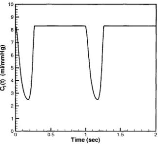
The key components of the model are the time-varying capacitors, which capture the pumping action of the heart. The two time-varying capacitors C,(t) and C1(t) represent the right and left ventricles of the heart. The contraction of the ventricles generates the pressure that drives the blood flow through the system. The capacitance waveform with respect to time for these capacitors is shown in Figure 1-2. The high-capacitance state is analogous to the relaxed diastolic state in the heart, while the low-capacitance state is analogous to the contracted systolic state of the heart's pumping cycle. The sudden drop in capacitance value, which corresponds to the contraction of the heart, causes the voltage across the capacitor to increase, thereby causing current to flow out of the time-varying capacitor and into the rest of the system. The rise in capacitance, which matches the relaxation of the ventricle, causes the voltage across the capacitor to drop, and marks the point where current begins to flow into the capacitor.

Two diodes separate each time-varying capacitor from the rest of the circuit. These diodes represent the valves between the atrium and the ventricle, and between the ventricle and either the pulmonary trunk (right ventricle) or the aorta (left ventricle). The diodes prevent the backflow of current in the circuit, just as valves in the heart prevent the backflow of blood in the system.

(19)

RAv _P th SM(C C (t h p Cup Rkidl _kd 2 TfCkid Ra CspR2 7 N~biasl P "sup C." Csu-I-Vh Rab p If ab Inf A I Pbasli,4 p'4

Figure 1-1: The circuit-based hemodynamic model.

plv pa Tpa - th Rr C,(t) th -0 P, I Ca

(20)

10 9 8 7 E 4 4 3 2 0 0.5 1 1.5 2 Time (sec)

Figure 1-2: Time-varying capacitance waveform.

The voltage sources labeled Pth simulate the intrathoracic pressure, which is a ref-erence for all the compartments within the chest; Pth varies in value with respiration.

The rest of the circulatory system is modeled with linear resistors and capacitors. In general, each capacitor represents a different compartment in the body. As we can see, the overall hemodynamic model captures the fact that the cardiovascular system is an interconnected circulatory system. Our figure omits various feedback control loops that the body uses the regulate the cardiovascular system. Specifics of parameter values and how the parameters were determined are described in Heldt's paper [3].

The transient response of heart rate to a stand test in the hemodynamic model is shown in Figure 1-3. The small ripples in the figure represent heart beats. The large, slowly varying transient curve is the response of the model to a perturbation of the system. When studying the cardiovascular system and its response to perturbations, such as lower body negative pressure or standing up, a cycle-averaged version of the hemodynamic model would appear to be sufficient to describe the average response over time. Circuit averaging is done because the local average behavior of a nearly

(21)

100 90 E ~80 cc C 70 -C) 60 -50' j 0 50 100 Time (sec)

(22)

periodic waveform is often the curve of interest when studying the general response over long periods of time. These time-averaged models become especially useful when the periodic ripples in heart-rate are not as important as the overall transient response. Most importantly, an averaged circuit can also be simulated and computed more efficiently and simply than the instantaneous case.

1.1.4 Time-Averaged Circuits

Circuit averaging is used in power electronics in order to analyze the dynamic behavior of many types of circuits containing switches that are operated in nearly periodic fashion. The idea involves using circuit techniques to develop a general averaged-circuit model that produces the local average response of variables within the averaged-circuit to any initial conditions or perturbations introduced to the system. Circuit averaging is often done in power circuits that contain switches and LTI (linear time invariant) components. A time-averaged version of a circuit should produce a response that captures the smooth variations in the local average behavior, with the switching ripple of the original response removed or attenuated. The cycle-averaged model should especially react similarly to the original model in its ability to follow the circuit's response to transients and perturbations. Often, it is these average values of voltages and currents in the circuit that are of interest during analysis. For example, when studying the transient response of the hemodynamic model, as in Figure 1-3, a time-averaged model would just capture the overall transient without the small periodic ripples. Circuit averaging can be done to increase computational efficiency. The averaged quantities are also the values needed for regulation and feedback control purposes.

Overall, the approach taken to developing a time-averaged circuit involves replac-ing all voltages and currents in the circuit by their cycle-averaged values, keepreplac-ing all the LTI components unchanged, and replacing the time-varying components in the system with appropriately chosen, and often approximate, equivalents [4].

(23)

1.2 Goals and Outline

This thesis will explore the characteristics of a simple version of the hemodynamic model, designed to represent a prototype cardiovascular circuit. Analysis and sim-ulation in HSPICE [1], a circuit analysis software tool, will be done to show the effectiveness of using HSPICE as a tool for analyzing computational models that involve potential-driven flows. Next, a cycle-averaged circuit based on the instan-taneous hemodynamic model will be designed to describe the average responses of our simple cardiovascular system. The motivation behind designing a cycle-averaged circuit includes computational efficiency. We will use HSPICE to characterize the time-averaged model and to show that it requires less computations than the instan-taneous case. Lastly, we will use the developed cycle-averaged model to analyze and simulate some feedback control loops present in cardiovascular dynamics within the body.

(24)

(25)

Chapter 2 A Simplified Model

The characteristics of the hemodynamic model are first analyzed piece by piece. The most unique and important feature of the model is the time-varying capacitor, a com-ponent that is not commonly seen in electrical circuits. Therefore, studies were first done with simulations in HSPICE of simple RC circuits with time-varying capacitors. Nodal analysis was performed for each of these preliminary models in order to un-derstand the characteristics of the time-varying capacitor. Finally, the pulsing simple heart model, which consists of a one-chamber heart, provides the primary circuit used to model a simple cardiovascular system. This pulsing model will be the basis for the time-averaged design.

2.1 Using HSPICE

The primary step in studying our computational model of the cardiovascular system involves implementing pieces of the system in HSPICE and studying the behavior of these components. HPSICE is a numerical circuit simulation tool. The current version of the hemodynamic model is not implemented in HSPICE. The motivation behind simulating such models in HSPICE includes the ability to take advantage of a developed and popular circuit design tool used by many engineers. As a highly developed program that is flexible and easy to use, HSPICE has the capability to implement complex circuits using very few lines of code. HSPICE is also designed to

(26)

solve all the equations necessary to plot and analyze the transient characteristics of any circuit model. All of the models described will be simulated and analyzed using this software tool [1].

2.2 A Simple RC Circuit

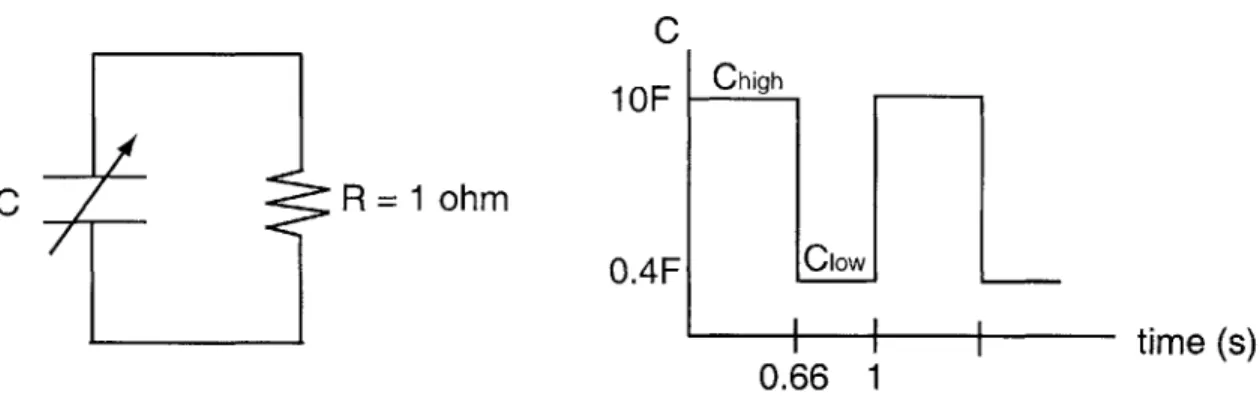
We begin by simulating in HSPICE a simple RC circuit with a time-varying capacitor. The circuit parameters are defined in Figure 2-1. The capacitance waveform has a

C

1

OF

C R = 1 ohm

time (s)

0.66 1

Figure 2-1: Simple RC circuit with time-varying capacitor.

period of 1 second, and is in the high capacitance (10F) state for 0.66 seconds and in the low capacitance (0.4F) state for 0.33 seconds. This waveform is an approximation to the capacitance waveform shown in Figure 1-2.

HSPICE has no direct implementation of a time-varying capacitor. However, it does allow the user to define a capacitance based on the voltage value at any node. The program written to implement the RC circuit with a time-varying capacitor defines a periodic voltage source separate from the rest of the circuit. This voltage source is controlled by a pulse function of defined amplitude, period, and duration to produce the desired time-varying waveform. The capacitance was then defined as a function of this voltage source. The HSPICE code for implementing the simple RC circuit is shown below:

(27)

RC Circuit * Title

.options post * Required

.op

** Initial voltage 10V across Capacitor

.ic V(ni)= 10

** Pulsing voltage source used to define the capacitance waveform

* Starts at 1bV, at 0.66s drops to 0.4V for 0.33s, repeats every is

Vcap n2 0 pulse(10 0.4 0.6666 in in 0.3333 1)

Rgrd n2 0 1meg

Cv n1 0 C = 'V(n2)' CTYPE=1 ** Define C interms of Vcap

R2 n1 0 1

**Transient analysis for 10s with timestep=0.Ois .tran 0.01s 10s UIC

.plot tran V(ni) .end

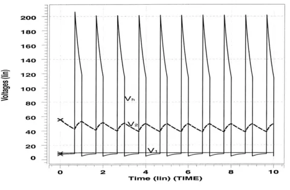
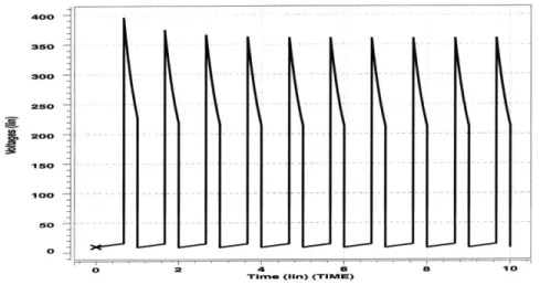
The circuit in Figure 2-1 was simulated with an initial voltage of 10V across the capacitor and produced the response shown in Figure 2-2. The response shows that the voltage peaks at the points in time when the time-varying capacitor drops in value from 1OF to O.4F. The drop in capacitance corresponds to a sharp increase in the voltage across the capacitor because the charge within the capacitor cannot change instantaneously (without impulsive currents). The voltage at the node decays after each peak since the capacitor discharges through the resistor when the capaci-tance value is constant. The heights of the voltage peaks also decrease with time, as

expected, since no additional charge is being placed on the capacitor by any sources

or recirculated to it from other capacitors. The circuit heads towards a steady state of OV at the node.

(28)

- - -q 2 40 - - -... .--. - -....- -.. -....

I,

220 200 10 IS0 140 120 100 so s0 40 20 0 0 2 11mnm (1in) (T-nIE) a 10

Figure 2-2: Simple RC circuit response to initial voltage of 10V, simulated in HSPICE.

2.3 Simple RC Circuit with a Current Source

Next, a current source of 100A was added to the simple RC circuit studied in Sec-tion 2.2. The circuit and capacitance waveform are shown in Figure 2-3. The current

C 1 OF

R = 1 ohm

O.4F

Figure 2-3: Simple RC circuit with a current source.

source supplies the circuit with additional charge. Therefore, the response of this system to an initial voltage of 10V does not decay to a steady state of OV as shown in Figure 2-4. Within two periods of the pulsing capacitance, the voltage across the

I = 100A C Chigh ClowI . 1 0.66 1 time (s)

-

-.

.

-

-.

.

-.

I

(29)

350 Soo mo0 10 50 0

Figure 2-4: Response of a simple RC circuit with a current source and initial voltage

of 1oV.

capacitor settles into a steady state with the voltage consistently peaking at around

360V at every transition to the Clow capacitance state. The nature of the time-varying

capacitance controls the periodicity of the voltage response behavior. During the Clo time interval, the voltage across the capacitor is high and it decays in value with a time constant of T = Clw* R = 0.4s as the capacitor discharges through the resistor.

In the Chigh time interval, the voltage is in a low state and it increases with a longer

time constant of Chigh * R = 10s as the capacitor stores charge from the current

source. Again, we can see how the time-varying capacitor coupled with a source of charge begins to capture the periodic, pulsing nature seen in the pumping behavior of the heart.

2.4 The Pulsing Heart Model

Next, a simplified version of the hemodynamic model was implemented in HSPICE. In this simple, single-ventricle, three-compartment model, shown in Figure 2-5, the central time-varying capacitor is analogous to the heart in the cardiovascular system.

(30)

R3 Ri Di D2 R2 Vh CV C Ca V2 +± Ri = 0.03 Q R2 = 0.01 Q CV= 100 F Ca = 2 F Cd = 10 F Cs = 0.4F Td = 0.66 s T = 1 s Cd Cs I I I I Td

T

Figure 2-5: The simple heart model with modeled on those in [3]).

capacitance waveform (parameter values

30 Vi C

time

I I

(31)

The diodes D1 and D2 are in place to prevent the backflow of current in the system.

These diodes represent the valves in the heart. The voltage V2 denotes arterial pres-sure; the voltage V represents the venous prespres-sure; Vh corresponds to the pressure within the heart; R3 is analogous to the resistance to blood flow in the body. This

simple model captures the behavior of a closed-loop circulatory system driven by a time-varying capacitor.

2.4.1 How it works

When C is in its high-capacitance state Cd, the voltage Vh is low. This corresponds to diastole when the chamber is in its filling state with a corresponding low heart pres-sure. During the diastolic portion of the cycle, the voltage V across the time-varying capacitor is low, current flows through the diode D1, diode D2 is non-conducting, and

Vh increases only slightly as charge is stored in C.

During the transition from diastole to systole, the heart contracts, causing the pressure in the heart to jump and blood to flow out of the heart. During systole in the circuit, C is in its low capacitance state and Vh is high. Consequently, current flows from the capacitor C through diode D2 into the rest of the system, and D,

becomes non-conducting. Therefore, Vh decreases in value as charge leaves the time-varying capacitor, corresponding to the behavior seen during the systolic cycle of the heart.

2.4.2 Simulation in HSPICE

The model in Figure 2-5 was implemented in HSPICE. The entire code for the circuit simulation is shown below:

Pulsing Heart Model * Title

.options post

.op

***Initial Conditions: Vi = 9V, Vh = 7V, V2 = 56V .ic V(n2)=9 V(n4)=7 V(n6)=56

(32)

***Define the voltage Source Vcap which implements the pulsing waveform

* for the time-varying capacitor:

Vcap nc 0 pulse(10 0.4 0.6666 lu lu 0.3333 1) Rgrd nc 0 1meg

***Define the Circuit Connections Cv n2 0 C = 100

R3 n2 n6 R = 1

R1 n2 n3 R =0.03

Ch n4 0 C = 'V(nc)' CTYPE=1 *Use the voltage source defined above R2 n5 n6 R =0.01

Ca n6 0 C = 2

D1 n3 n4 diodel

D2 n4 n5 diodel

.model diodel D level=1 IS=le-14 CJO=le-12 VJ=.783

***Transient Analysis over 10s with steps of 0.Ols

.tran 0.Ols 10s

.end

These few lines of code define the connectivity between the parts of the model, the initial conditions, the type of analysis, and the pulsing capacitance waveform. Due to

the pulsing capacitance, we will henceforth refer to this model as the pulsing model.

Figure 2-6 shows the simulation of the pulsing model using the initial values V1 = 9V, Vh = 7V, V2 = 56V. Since the capacitance C starts off in the diastolic

state, the initial value of Vh was chosen to have a low value compared to V and V2.

The plots of the voltages at each node follow the expected characteristics.

All of the waveforms are periodic with a period of T = 1s. The first 0.66 seconds of each period correspond to a state of diastole where Vh, corresponding to the pressure in the heart, is low compared to V1 and V2. The voltage Vh grows with an approximate time constant of Cd * R, = _{0.3s as current flows through the diode D}₁ _{and into the} capcitor C. During diastole, no current flows through R2 since diode D2 is non-conducting. However, charge does leave the capacitor Ca through R3, causing V2 on

(33)

0 2 4 6

TIme (iiri) (TIMVU)

8

Figure 2-6: Simulation of the pulsing model in HSPICE.

ao 200 --18O 16O 140 120 100 8o 60 40 20 0 h .. . -. ... 10

(34)

C, is so large, the voltage V on the venous side remains relatively constant. By the end of diastole, the voltage Vh is approximately equal to V1.

The last 0.33 seconds of each period correspond to the state of systole in the heart. During systole, Vh is very large, causing the diode D2 to start conducting and diode

D1 to become non-conducting. Current flows from capacitor C through R2 with a

fast time constant of about R2 * C, = 0.004s. This fast time constant produces the

sharp peaks seen in Figure 2-6. The fast time constant also causes Vh to drop rapidly until it equals V2. When Vh equals V2, they both start decreasing with a time constant

of about R3 * Ca = 2s as Ca discharges through R3. At the end of one period, the

circuit switches back to the diastolic state, causing the cycle to repeat. Note that the very high peaks of the Vh curve are not seen in an actual physiological response of the cardiovascular system. The sharpness of the peaks are due mainly to the small values of R2 and C, and the abrupt step changes in the capacitance waveform.

The charge q stored in a capacitor C with voltage Vh is given by:

q = CV (2.1)

At the step change in C from Cd to C8, the pulsing model switches from the diastolic

to the systolic state. The sudden change in C causes a sharp change in the value of

Vh since the charge stored in the capacitor remains constant during the transition.

At the transition from Cd to C8, Vh sharply increases from Vh(-) to Vh(+) = Vh(-)CdC.,

i.e.,to 40 times its diasolic level. At the transition from systole back to diastole, C steps from C, to Cd and Vh drops to 0.04 times the value it was at the end of systole. After one to two periods, the simulation essentially falls into a steady state where Vh peaks at the same value of 193V every cycle.

2.4.3 Changing R2

When the resistor R2 in the pulsing model is increased from O.O1Q to 1Q, the circuit

produces the simulated behavior shown in Figure 2-7. This increase in R2 could be

analogous to high resistance in the outlet valve of the heart, which could result from 34

(35)

aortic stenosis. The differences between Figure 2-6 and Figure 2-7 are pronounced. The increased vascular resistance causes a slower decay of the voltage Vh across the time-varying capacitor. As a result, the peaks in Vh are not as sharp and the rise time of V2 on the arterial side is much slower.

Ca 200 180 160 140 120 100 80 60 40 20 0 0 2 4 6

Time (lin) (TIVI)

8 10

Figure 2-7: Simulation of the pulsing model with a larger value of R2 = 1Q.

2.5 Using the Pulsing Model

The pulsing model will be the basis for the time-averaging of circuit variables and the development of the cycle-averaged model. The model is simple enough that there are only a few circuit variables and parameters to study, but it can still model the basic characteristics of a cardiovascular system. A cycle-averaged version of the pulsing model should be computationally more efficient and should capture the transient responses of the system to disturbances or perturbations.

(36)

(37)

Chapter 3 Developing the Cycle-Averaged

Model

The goal of a cycle-averaged model is to capture the overall cycle-to-cycle transient behavior of a given heart model while supressing the intra-cycle details. The key to developing such a model is to replace the time-varying capacitor and the diodes in the heart model with elements that only depend on cycle-averaged quantities within the circuit. The design should produce time-averaged responses that are smoothed, averaged curves without the sharply pulsatile nature of the detailed pulsing heart model responses. The cycle-averaged model will be more computationally efficient when intra-cycle details are not of interest, and can be used to define control struc-tures within the system that only involve locally averaged rather than instantaneous variables.

3.1 Introduction of a Transient

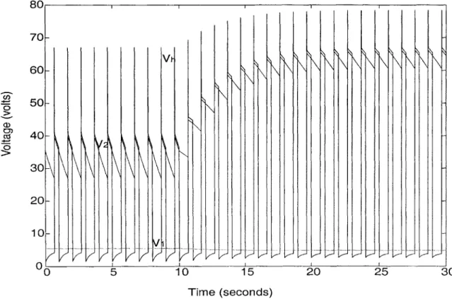
In order to study the time-averaged response to changes within the system, a transient was introduced to the pulsing heart circuit of Figure 2-5. This transient was produced

by a step at 10 seconds in the resistance R3, from 1Q to 5Q. The response of the model to the step in resistance is shown in Figure 3-1. The step increase in resistance produces an increase in the average values of the voltages Vh and V2. This transient

(38)

will be used to analyze the behavior of the time-averaged model. 8 0 1 1 i C,, 0 CZ 70 60 50 40 20 10 0' ) 20 25 Vt

-

V

Time (seconds)

Figure 3-1: Response of the pulsing model to a transient in R3.

3.2 Calculating the Time-Average Waveform

The (symmetric) cycle-averaged value of a waveform V is a time-average over each period T of the cycle, and is defined by:

=T < V(t) >

=+-Tt- T

V(T)dT . (3.1)

A property of this definition is that:

dV\ d_ <V>

dt dt (3.2)

The cycle-averaged waveforms of Vh and V2 from the transient responses in Fig-30

(39)

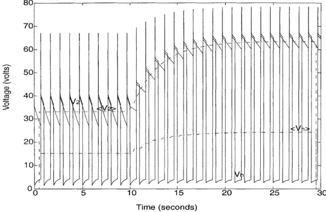
ure 3-1 were calculated in MATLAB using the trapezoidal rule to approximate the in-tegral in Equation 3.1, with a timestep of 0.01 seconds. The calculated time-averaged waveforms are shown as the dotted lines < V1 > and < V2 > in Figure 3-2. These

80 1 1 1 1 I 70 - 60- 50-40 30 20 10 01 C

I

I V I 'i LJ I/ VKKK VK 5 0 15 Time (seconds) /I~ 20 25 30

Figure 3-2: The calculated time-averaged waveforms of Vh and V2.

curves are generally smooth and lack the pulsatile nature of the original voltage wave-forms. The slight ripples in the curve near the transient are due to the non-periodicity of the waveforms during the transient. (The zero values at the beginning and end are from the limitations to the time-frame used in HSPICE.) During the change in R3, the calculated cycle-averaged voltages < Vh > and < V2 > increase in value, consistently with the behavior seen in the original model.

The cycle-averaged circuit models that we are aiming to develop should produce

responses that are good approximations to the cycle-averaged waveforms in Figure

3-2 for this same experiment (namely, a step change in R3), as well as in other such

experiments. Therefore, during the development of the cycle-averaged model, the

1-1

0

_11x

/I- I-, [I--, _

(40)

results we obtain will be compared to this calculated average.

3.3 Finding

Ceff

In order to create a cycle-averaged model, we first study how to replace the time-varying capacitor in the pulsing model with a constant, effective capacitance value.

3.3.1 Calculations with Elastance

It will be more convenient for our purposes to work with the reciprocal of capacitance, namely elastance,

1

C

For the time-varying capacitance waveform seen in Figure 2-5 in Chapter 2, we can draw the elastance waveform as in Figure

E

3-3. We will make use shortly of the

1/Cs 1 /Cd T Td Ts time Time in Systole: Ts = T -Td Time in Diastole: Td

Figure 3-3: Time-varying elastance waveform.

time-average of this elastance waveform, or the effective elastance, namely 1 T Td Cd (3.4) 40 (3.3) I + -T. CS

(41)

Since V = Eq from the combination of Equations 2.1 and 3.3, where q is the charge on the capacitor, taking the time-averaged values produces:

< V > = < Eq > (3.5)

The charge q has relatively low ripple, and is approximately constant compared to E over any interval of length T. We can therefore make the approximation

< V > r < E >< q > . (3.6)

The current through a constant capacitance C is given by

dq(t) dV 1 dV

)_ - . (3.7)

dt dt E dt

The time-average of the current can then be written as:

< > = d(t) (3.8) dt d (< V >) ₃₉ - (3.9) dt <E > 1 d - d < V > . (3.10) < E >dt

Equation 3.8 follows from 3.2, Equation 3.9 follows from 3.6, and 3.10 follows because

< E > is constant since E is periodic. Since the result in Equation 3.10 is similar

to the expression for current in Equation 3.7, and is in the form expected for a time-averaged circuit, one possibility for replacing the time-varying elastance would be to use < E >, the time-averaged value of the elastance E. Therefore, in a cycle-averaged circuit model, the equivalent elastance of the time-varying capacitor would be the value of < E > in Equation 3.4. The corresponding effective capacitance is

Ceff = .T3.1

(42)

3.3.2 Ceff in a Simple RC circuit

A simple RC circuit similar to the one described in Chapter 2, Section 2.2 was used

to analyze the behavior of a system which incorporates the value of Ceff. First, the simple RC circuit with a step change in resistance at 6 seconds, shown in Figure 3-4, was simulated in HSPICE. The response with a time-varying capacitor C is displayed as the pulsing waveform in Figure 3-5 . The step change in resistance caused the voltage to increase with an exponential transient. The time-average response was calculated and is depicted as the dotted line in Figure 3-5.

I = 100A C R = Step at 6s from 1ohm to 5 ohm C 1 OF O.4F Chigh Clow I I 0.66 1 time (s)

Figure 3-4: RC circuit with a step in resistance.

Next, the time-varying capacitor in Figure 3-4 was replaced with a constant ca-pacitance. Four simulations were done, each with a different constant capacitance value. The values chosen include the high capacitance value Chigh, the low capaci-tance value Clow, the average value of the high and low capacicapaci-tances Cag, and the effective capacitance Ceff derived from the time-averaged elastance and specified in Equation 3.11. The values are displayed in Table 3.1. The simulation with each of

Capacitance Value

Chigh lOF

Cow

O.4F

Cavg 5.2F

Ce!! 1.11F

(43)

70C 1 1 - Calculated <V: Using Ceff - Using Cavg

60C

50C- 40C-CD) 0 a) o 30C-20C- .- 9oN loc-10C - - -- - - -20~ 0

2

4 6 8 10 12 Time (Seconds)

(44)

these values is shown in Figure 3-5. We can see that the curve which results from us-ing the value of Ceff most closely matches the calculated time-average of the original voltage < V >.

To exhibit the behavior of Ce!f for other types of transients, the RC circuit in Figure 3-6 with an exponentially varying current source was simulated. The expo-nential current source provided the transient in the circuit. This expoexpo-nential function increased with a time constant of is towards a value of lOGA and at t = 2s fell with a time constant of 2s back towards GA. The voltage waveforms derived from simulation of this circuit are displayed by the pulsing curve in Figure 3-7. The plot shows

os-I = exp(O 100A 0 ls 2s 2s) _C

10F Chigh

S

C

/

R=1ohm

I

0.66 1 time (s)

Figure 3-6: RC circuit with an exponential current source.

cillations in the voltage across the time-varying capacitor. The general response also captures the exponential nature of the current source. The calculated time-average of the voltage is plotted as the dotted line. The response of the same circuit, except with a constant capacitance of Ce!f equal to 1.11F in place of the time-varying

ca-pacitor, is shown as the solid curve. Again, replacing the time-varying capacitor by a constant capacitance Ce!! produces a circuit that follows the time-average of the voltage curve. This result further solidifies the reasoning behind using Ceff as the

(45)

300 II I II - Original - Calculated <V-Using Ceff 25C- 20C-U) a0) 1

50-V from Circ jit with Ceff

0

0 2 4 6 8 10 12

Time (Seconds)

(46)

3.4 Replacing the Diodes

The next step in developing a cycle-averaged circuit model involves replacing the diodes in the original pulsing model, shown again in Figure 3-8, with elements that

depend only on averaged variables within the circuit.

R3 Ri = 0.03 Q R1 D1 D2 R2 1R2 = 0.01 Q V1iV V2 R3 = 1 92 Cv = 100 F Ca = 2 F CV Vi

/

C V Ca Cs = 0.4F - Td = 0.66 s T=1 s C Cd Cs i Itime Td T

Figure 3-8: The pulsing model.

3.4.1 Voltage Analysis with Switching Functions

In order to characterize the voltages across each diode, the voltages Vi and V in Figure 3-8 of the pulsing model were studied. Each diode is in one of two states: con-ducting or non-concon-ducting. During diastole, diode D, is concon-ducting current while D2

is non-conducting. During systole, diode D1 is non-conducting and D2 is conducting.

We also define two switching waveforms q and q' = 1 - q as shown in Figure 3-9.

The waveform q is 1 during the diastolic portion of the cycle, while q' is 1 during the 46

(47)

q q' 1 1 0 time 0- time Td T Td T Ts Ts Td = 0.667 seconds Ts = 0.333 seconds T = 1 second

Figure 3-9: Switching functions q and q'.

systolic part of the cycle. Also we denote the (constant) time-average value < q >

by a and < q' > by a'; note that a is the fraction of each cycle that the heart is in

diastole. For the parameter values in Figure 3-9, a equals 0.667 and a' equals 0.333. The voltage Vi equals the voltage Vh across the time-varying capacitor during diastole when the diode Di conducts current, and equals V during systole when D1

is non-conducting. This relation is described using Equation 3.12:

V, qVh + qV1 (3.12)

For a heart rate of 1 cycle/second with the values of Td = 0.66s and T, = 0.33s, Equation 3.12 says that the voltage Vi is equal to Vh during the first 0.66 seconds of the cycle, and is equal to V during the last 0.33 seconds of the cycle.

Similarly, the voltage V equals Vh during systole when D2 is conducting, and

equals V2 during diastole when D2 is turned off. This produces Equation 3.13:

V = qV2 + q'V . (3.13)

Taking the cycle-average of Equations 3.12 and 3.13 gives us:

(48)

<VO > = < qV2 > + < q'Vh > .(

These equations will become useful in building the cycle-averaged model. What we seek are approximations that allow the averages of products, as on the right sides of Equations 3.14 and 3.15, to be written purely in terms of single averaged variables.

3.4.2 Current through the Diodes

The current through diode D1 equals the current il through resistor R1 at all times,

and the current through diode D2 equals the current 12 through R2. The current i1

is zero during the systolic phase of the cycle, and the current i2 is zero during the

diastolic portion of the cycle. We shall find an approximate expression for < i1 >

below.

3.5 The Preliminary Cycle-Averaged Model

We begin by using the waveforms for Vh, V1, and V2 seen in Figure 3-10 to make

approximations to the equations describing the time-averaged voltages, < V > and

<

Vi >, and the currents, < i > and < i2 >. Note first that because C, is so large, V is essentially constant over any interval of length T, so we shall feel free to replace Vi by < V > in all that follows.

3.5.1 Time-averaged Current

Plotting a couple of periods of the Vh cycle in steady state, shown in Figure 3-10, helps describe the current il based on other variables and parameters in the pulsing model.

If we assume that during systole Vh decays with a fast time constant (T ₌_0.004s)

towards V2, then early in systole V becomes equal to the value of V2. If we denote the

value of Vh at the end of systole by Vhsy, and its value at the beginning of diastole by

Vhdia, then V1hda = - Vhy, since the time-varying capacitor changes in value from C, to Cd. We can then describe the initial current, iinitiaI, through D₁ at the beginning

(49)

3.5 4 4.5 5

Time (seconds)

Figure 3-10: Closeup of key waveforms.

200 180-16C 14C 12C 10C 80 C,) 0) (C, 0 diastole Vhsys V2 Vh Vhdia Vi 60 40 20 0 3 5.5

----

---

----

--

-systole diastole

(50)

of diastole to be: . V1 - Vhdia (3.16) V - CsVsys 1 -d (3.17) R, V1Cd - VhsysCs (3.18) RjCd

This current decays during diastole with a time constant of T RlCd= 0.3s. So the

current i1 during the diastolic state can be written as:

i1(t) = (VlCd-VhsysCs) e RCd (3.19)

Note that i1 only flows during diastole. Also, the value of Vsys is approximated

as being equal to < V2 >, the average value of V2. This approximation is based on

the assumption that V2 has relatively low ripple and is perhaps the poorest of the

approximations we make, given that V₂has a 25%-30% peak-to-peak ripple. Better approximations can be made, at the cost of making the model somewhat more com-plex, but these refinements are left to future work (see Appendix B for a preliminary study). If we assume that by the end of diastole the current il has essentially decayed to zero, with Vh essentially equal to V1, we can compute the time-averaged current as: I aT VCd - VhsysCs < = T (VlCd )e Rj~d dT (3.20) < V1 > Cd- < V2 > Cs R1Cd ~ V Cd )RTd(3.21) < V1 > Cd - < V2 > Cs

_3.2

(3.22) T 50

(51)

3.5.2 Time-averaged Voltage V

Next, using Equation 3.15 and considering the waveform V2 in Figure 3-10 to be

relatively low ripple, we approximate:

< V > ~ a < V2 > + < q'Vh> . (3.23)

Furthermore, the time-average < q'V > is the same as:

< q'Vh > < Vh> - < qV> . (3.24) During diastole, the voltage V/ rises exponentially, with a time constant of 0.3s, to meet the value of V seen in Figure 3-10. Estimating that V is a relatively small, constant value, we then make the preliminary approximation:

< qVh > ~~a < V> - (3.25)

Combining these approximations gives an expression for < V, >:

<V> ~ <V2 >+<Vh> -a<Vl > . (3.26)

3.5.3 The Initial Three-Source Cycle-Averaged Model

The initial cycle-averaged model proposed is shown in Figure 3-11. This model cap-tures the desired average current flow through the circuit by placing the dependent current source I, between the capacitors C, and Ceff. The value of Ceff was de-rived in Equation 3.11 and calculated to be 1.11F, and I is given by the average value < i1 > determined in Equation 3.22. The dependent source V, captures the

value of < V > given in Equation 3.26, and the current source I, simply follows the time-averaged current < i2 > through R2. Combining these with the circuit values introduced in the pulsing model shown in Figure 3-8, the definitions of the dependent

(52)

<i3> <i1> * <Vh> R2 <2> <V1 > <V2> CV Ceff + Ca la Va Is = (Cd<V1> - Cs<V2>)/ T R2 = 0.01 Q

la = <i2> R3 = 1 -5 Q (Step at 1 Oseconds)

Va = CC<V2> + <Vh> - c<V1> Cv = 100 F Ca =2 F Cen = 1.11 F Cd = 1OF Cs = 0.4F a= 0.66 T = 1 s

(53)

sources in Figure 3-11 are numerically: Va a < V2 > + < V > -a < V1 > = 0.66 < V2 > + < Vh> -0-66 < V > = < i2 > Is =< i >= (3.27) (3.28) (3.29) (3.30) (3.31) Cd < V > -Cs < V2 > T = 10 < V1 > -0.4 < V2 > .

3.5.4 Simulation of the Three-Source Model

The three-source model depicted in Figure 3-11 was simulated in HSPICE using initial conditions closer to the steady state values in diastole, with < V > at 5.56V, < V1 > at 1.45V, and < V2 > at 35.4V (Appendix A). The response of the voltage < V1 > in the model is shown in Figure 3-12 (solid line) along with the calculated time-average of the voltage waveform Vh from the pulsing model (dotted line). The response

-Calculated <Vt>

1)

K IL II

$11

ii

I*i~

I

VI

_________ V

u t dkh h> frI 3 soy! ecr - 1ce oe00

tC l=t~LH

~0 5 10 15 20 25 30

Time (seconds)

Figure 3-12: The response of voltage < Vh > in the Three-Source Time-Averaged

Model.

follows the general shape of the calculated time-average values. During the transient

70 60 50 40 3C 2C 1iC * D It (7 M I

Cycle-averaged models of cardiovascular dynamics

Cycle-Averaged Models of Cardiovascular

Dynamics

by

Jolie L. Chang

Submitted to the Department of Electrical Engineering and Computer

Science

in partial fulfillment of the requirements for the degree of

Master of Engineering in Electrical Engineering and Computer Science

at the

MASSACHUSETTS INSTITUTE OF TECHNOLOGY

June 2002

@

Jolie L. Chang, MMII. All rights reserved.

The author hereby grants to MIT permission to reproduce

Ud

distribute publicly paper and electronic copies of this thesis document

in whole or in part.

Author .

JUL

3 1 2002

LIBRARIES

BARKER

Department of Electrical Engineering and Computer Science

May 24, 2002

Certified by ...

George C. Verghese

Professor

.Thnis Supervisor

Accepted by ...

:.

.

...

Arthur C. Smith

Chairman, Department Committee on Graduate Students

Cycle-Averaged Models of Cardiovascular Dynamics

by

Jolie L. Chang

Abstract

Acknowledgments

Contents

List of Figures

List of Tables

Chapter 1

Computational Models and

Biological Systems

1.1

Background and Previous Work

1.1.1

The Cardiovascular System

1.1.2

Modeling the Cardiovascular System

1.1.3

The Computational Hemodynamic Model

1.1.4

Time-Averaged Circuits

1.2

Goals and Outline

Chapter 2

A Simplified Model

2.1

Using HSPICE

2.2

A Simple RC Circuit

OF

time (s)

I,

2.3

Simple RC Circuit with a Current Source

-

-.

.

.

.

.

.

.

.

.

.

_3.2