HAL Id: cea-00853368
https://hal-cea.archives-ouvertes.fr/cea-00853368
Submitted on 2 Oct 2020
HAL is a multi-disciplinary open access
archive for the deposit and dissemination of
sci-entific research documents, whether they are
pub-lished or not. The documents may come from
teaching and research institutions in France or
abroad, or from public or private research centers.
L’archive ouverte pluridisciplinaire HAL, est
destinée au dépôt et à la diffusion de documents
scientifiques de niveau recherche, publiés ou non,
émanant des établissements d’enseignement et de
recherche français ou étrangers, des laboratoires
publics ou privés.
monitoring networks: The European flux tower network
example
Mika Sulkava, Sebastiaan Luyssaert, Sönke Zaehle, Dario Papale
To cite this version:
Mika Sulkava, Sebastiaan Luyssaert, Sönke Zaehle, Dario Papale.
Assessing and improving the
representativeness of monitoring networks: The European flux tower network example.
Jour-nal of Geophysical Research: Biogeosciences, American Geophysical Union, 2011, 116, pp.G00J04.
�10.1029/2010JG001562�. �cea-00853368�
Assessing and improving the representativeness of monitoring
networks: The European flux tower network example
Mika Sulkava,
1Sebastiaan Luyssaert,
2Sönke Zaehle,
3and Dario Papale
4Received 30 September 2010; revised 27 January 2011; accepted 11 February 2011; published 17 May 2011. [1]
It is estimated that more than 500 eddy covariance sites are operated globally,
providing unique information about carbon and energy exchanges between terrestrial
ecosystems and the atmosphere. These sites are often organized in regional networks like
CarboEurope
‐IP, which has evolved over the last 15 years without following a predefined
network design. Data collected by these networks are used for a wide range of
applications. In this context, the representativeness of the current network is an important
aspect to consider in order to correctly interpret the results and to quantify uncertainty.
This paper proposes a cluster
‐based tool for quantitative network design, which was
developed in order to suggest the best network for a defined number of sites or to assess
the representativeness of an existing network to address the scientific question of interest.
The paper illustrates how the tool can be used to assess the performance of the current
CarboEurope
‐IP network and to improve its design. The tool was tested and validated with
modeled European GPP data as the target variable and by using an empirical upscaling
method (Artificial Neural Network (ANN)) to assess the improvements in the ANN
prediction with different design scenarios and for different scientific questions, ranging
from a simple average GPP of Europe to spatial, temporal, and spatiotemporal variability.
The results show how quantitative network design could improve the predictive capacity
of the ANN. However, the analysis also reveals a fundamental shortcoming of optimized
networks, namely their poor capacity to represent the spatial variability of the fluxes.
Citation: Sulkava, M., S. Luyssaert, S. Zaehle, and D. Papale (2011), Assessing and improving the representativeness of monitoring networks: The European flux tower network example, J. Geophys. Res., 116, G00J04, doi:10.1029/2010JG001562.
1.
Introduction
[2] Since the first successful measurements of the net CO2
exchange between forest and atmosphere [Baldocchi et al., 1988], eddy covariance (EC) based methods have gained popularity and have become one of the central observational tools at more than 500 sites around the world [Baldocchi, 2008]. These data have been increasingly used to support regional and global analyses of CO2, water and energy
exchanges between terrestrial ecosystems and the atmo-sphere [e.g., Beer et al., 2010; Ciais et al., 2005; Piao et al., 2008; Valentini et al., 2000]. However, this network of sites was never formally designed; that is, new towers were not necessarily established at locations that represented a gap in the network. Instead, site selection was based on feasibility and previous experience. As a result, accessibility, logistics
and topography suitable for EC measurements were major determinants for site selection.
[3] As an example, while over 100 sites were established
in Europe, often in the context of European coordinated projects, with the exception of a few large institutes, most sites were managed by individual research groups. The European network went through several cycles of self‐ organization. After a first phase of focus on forest ecosys-tems the network was extended with grassland, cropland and wetland sites subject to different management practices. Later, sites were added in the more extreme climate condi-tions of northern and southern Europe and following the expansion of the EU itself, Eastern European partners were taken onboard. The network is currently believed to cover the most important land uses of the dominant climate zones. However, it does not by any means cover the full botanical, environmental and edaphic diversity, nor the variety of disturbances and management strategies found at the Euro-pean continent. Although some regional clusters of sites were established to study the effect of land use change or land management, the network as a whole lacks a formal experimental design.
[4] In parallel with the more fundamental research that
seeks to better understand the carbon and water cycle of terrestrial ecosystems, international commitments to reduce
1Department of Information and Computer Science, Aalto University
School of Science, Espoo, Finland.
2
Laboratoire des Sciences du Climat et de l’Environnement, CEA, CNRS, UVSQ, Gif‐sur‐Yvette, France.
3
Max‐Planck‐Institute for Biogeochemistry, Jena, Germany.
4Department of Forest Environment and Resources, University of
Tuscia, Viterbo, Italy.
Copyright 2011 by the American Geophysical Union. 0148‐0227/11/2010JG001562
CO2emissions (Kyoto) require that the self‐declared
emis-sion reduction be verified by atmospheric measurements [Nisbet and Weiss, 2010]. In Europe, the dense network of EC towers appears as a powerful source of information to complement the observations of a network of atmospheric stations monitoring the changes in atmospheric CO2
con-centrations (i.e., the ICOS initiative). However, the use of the existing EC network to inform priors for emission verification is hampered by, among other things, its lack of design and therefore its ill‐defined or better, unknown representativeness.
[5] In general terms, the representativeness of a network
can be defined by its ability to reproduce the main (statis-tical) characteristics of quantities or processes of the popu-lation under study. An optimal sampling network represents the characteristics of the population while avoiding redun-dancies. From a more practical perspective, this implies that sampling network should be constituted by measurement stations (i.e., EC towers) in as many different conditions as possible. In the example of an EC network, conditions can either refer directly to the quantity or process of interest or its drivers or parameters, in which case, network design becomes a multidimensional task. For multidimensional problems, clustering techniques, as applied in this study, have been shown to be useful for characterizing multidi-mensional environmental data [Luyssaert et al., 2004] and quantifying the representativeness of particular locations [Hargrove and Hoffman, 1999].
[6] There have been attempts to assess the
representa-tiveness of an existing flux tower network. Hargrove et al. [2003] studied the American EC network and the impact of the actual design on specific analysis using a GIS approach that identified areas with similar characteristics in respect to climate, soil and disturbances based on stratification of the environmental data space using k‐means clustering. The same methodology was applied in the initial design of the National Ecological Observatory Network (NEON) in the United States [Schimel et al., 2007].
[7] Furthermore, minimum distance approaches have been
used for empirical and model‐based upscaling. The model parameters used at each pixel were taken from the most similar EC site of the European network, where the para-meters were estimated using the measurements [Carvalhais et al., 2010]. That study used a nearest neighborhood clas-sification of the climatic and phenological conditions in order to quantify the multidimensional distance in data space between each pixel and the sites. Jung et al. [2009] studied the effect of the actual network design in the con-text of an empirical upscaling exercise. For upscaling, a machine learning approach making use of model simula-tions was applied to show the ability of machine learning to reproduce monthly gross primary production (GPP) of the globe when the learning algorithm was parameterized using only data extracted at the locations of existing observational stations.
[8] The current paper presents a tool for evaluating the
representativeness of the current European EC network and proposes possible improvements to the network design with the longer‐term objective of designing the EC network in such a way that allows it to become a powerful component of a monitoring system able to track changes in the bio-sphere‐atmosphere exchanges. The proposed quantitative
network design (QND) tool can deal with the three fol-lowing general network design questions: (1) How repre-sentative is an existing network and in which regions does the network perform poorly? (2) Where should measure-ment stations be added or removed in order to optimize an existing network? (3) How should a new network of mea-surement stations be designed so that it is optimal in the sense that it contains the minimal number of stations to obtain a specific precision and accuracy for its objectives (see below) and represents all relevant ecological char-acteristics represented (e.g., major ecosystem and vegetation types)?
[9] The network design question is closely linked to the
objectives for which the observations of the network are used. Examples of the objectives that have been and may be studied with data from the EC network include cross‐site synthesis activities addressing issues in ecophysiology, ecology, model development, ecosystem model parameter-ization and validation, as well as upscaling of ecosystem fluxes to larger spatial scales. This study has worked toward developing a tool that enables its users to quantitatively analyze the current network and optimize its design for future use.
[10] In order to demonstrate and validate this tool, its
possibilities, limitations and interpretation, four realistic network objectives were selected with increasing computa-tional complexity. These objectives were to monitor the mean, spatial variability, semivariance and spatiotemporal variability of gross primary production (GPP). The four objectives were applied in order to evaluate the represen-tativeness of the current network and suggest how its design could be improved to better study the same objectives in the future. Validation of the QND tool required knowledge of the target spatial explicit variable. As a target quantity, the study used the GPP simulated by means of a biogeochem-ical model as a substitute of the true but unknown GPP.
[11] The specific objectives of the paper are as follows:
(1) show how the choice of objectives of the network affects the apparent representativeness of the current network, (2) identify the regions of Europe where the current network is uncertain (depending on the objectives; 2.3.1) and (3) quantify the degree to which this uncertainty could be reduced by network optimization.
2.
Methods
2.1. Features of the Quantitative Network Design Tool [12] A quantitative network design (QND) tool was
developed that can be used to answer the three following distinct design questions: (1) Is an existing network of measurement stations representative for its objectives and consequently, which areas are less represented and therefore have a higher uncertainty? (2) Where should measurement stations be added or removed in order to optimize an existing network for its objectives? (3) How can a new network of measurement stations be designed so that it is optimized for its objectives (that is, the minimal number of stations needed to obtain a specific precision and accuracy for its objec-tives)? The most important features of such a tool, from a user’s point of view, are listed below.
[13] 1. Based on a number of spatially explicit data (e.g.,
character-istics, remotely sensed data, and model output), the QND tool analyzes the representativeness of an existing moni-toring network, highlights the areas that are currently less represented, or optimizes the monitoring network in order to cover the maximum variability contained in the spatially explicit data. The tool is independent of spatial and temporal scale; it can be used at the global, continental, regional, landscape or site level depending on the spatial scale of the input data. Similarly, it can be used at decadal, annual, seasonal, monthly, weekly, daily or hourly levels depending on the temporal resolution of the input data
[14] 2. Choosing the spatially explicit data to be used in
network evaluation or network design is critical, as these data must fully represent the process or application under study. If, for example, the representativeness analysis is performed in order to improve the quality of an upscaling model, the data used in the network evaluation should be the same as the input of the upscaling model. If, however, the analysis aims to study the representativeness of the network in terms of climate variability, the inputs could be maps of variability (e.g., standard deviations) of the different mete-orological data. Consequently, data space in terms of the variables and number of variables is defined by the user. However, all variables should have the same spatial and temporal resolution.
[15] 3. The underlying algorithm does not formally
require the spatially explicit input variables to be indepen-dent. However, all variables are considered equally impor-tant and, therefore, are processed with the same weight. Consequently, using strongly related variables will result in a network that better represents the related variables. For example, a network study based on air temperature and precipitation will result in a network that is equally repre-sentative for both variables. If, however, a similar network is designed for precipitation, air temperature and soil temper-ature, the network will better represent the variability in temperature than in precipitation because two strongly related temperature variables were used.
[16] 4. The QND tool has the option of using one variable
to create distinct strata; for example, different plant func-tional types or administrative units. In this case, the different strata are treated as independent with respect to each other and the algorithm has the innovative feature of ensuring representation of each of the strata based on the input variables and the towers that already represent the strata. The tool treats all strata simultaneously and the user can choose from two options for allocating towers to strata. The first option involves adding a tower to the stratum where the new tower results in the largest absolute uncertainty reduction, while the second adds a tower to the stratum with the highest uncertainty of all strata. Adding a new tower reduces this uncertainty. Towers are added to this stratum until its uncertainty drops below that of one of the other strata.
[17] 5. In order to analyze the representativeness of an
existing network, the locations of measurement stations within the network are given. When the tool is used to design an optimal network, the user should specify the maximum number of sites based on, for example, financial constraints or a quantitative measure of precision or accu-racy the network should reach.
[18] 6. When the tool is used to optimize an existing
network (design question 2, above), the analysis takes the existing sites and their location into account. For each sta-tion, the user must specify whether the station is mandatory in the optimized network. A mandatory station is a site that, even if it is not optimally located for the objectives of study, is retained in the network. It may be desirable to retain suboptimal stations because of other aspects, such as fund-ing, length of the time series, and completeness of the data. When designing a network with many mandatory stations, more stations will be required in total in order to obtain the same representativeness level as with a network without mandatory stations. Nonmandatory stations are only retained when their representativeness exceeds the threshold of a user‐ specified representativeness measure. User‐specified repre-sentativeness measures can be defined in many ways but they are all technical (and are therefore dealt with in section 2.2.3). 2.2. Workflow and Principles of the Quantitative Network Design Tool
2.2.1. Workflow of the QND Tool
[19] The QND tool builds on recent progress in cluster
analysis. A novel feature of the tool is that spatially explicit input data are clustered in order to obtain groups of locations with similar values for the different variables. The cluster center is the location that best represents the whole cluster because it has the smallest total distance, in terms of data space, to all members of the cluster. The QND will rec-ommend pixels with characteristics similar to the cluster center as the sampling station. The cluster center is a sta-tistical feature of the data and does not necessarily exist in situ. Hence, sampling locations will be proposed at in situ locations with characteristics that are as similar as possible to the clusters’ centers.
[20] The representativeness of an existing network is
dependent on the distance, measured in data space, between the cluster centers and the established stations. This is a typical phenomenon in predictive modeling in which func-tions are interpolated and extrapolated using models that are not entirely correct. In this respect, it is unlikely that any model of a complex natural system would be correct [Shapiro, 1998]. When the data are rather smooth, i.e., when small changes in drivers do not produce large changes in fluxes, the uncertainty of the model can be assumed to be proportional to the difference of the values of the variables to those observed at the sampling stations. An important feature of the proposed QND tool is that it does not assume any specific model for the ecosystem [cf. Law et al., 2004]. [21] Irrespective of whether representativeness or design
questions need to be addressed, the QND tool follows the same workflow. However, depending on the question under study, some of the quantitative results of a previous task are not used. The order of the tasks within the QND tool is as follows.
[22] 1. Define the scientific question to be answered by
the network, select the appropriate input and related char-acteristics (e.g., temporal and spatial resolutions) and decide if the analysis should consider different strata and, if so, define them (e.g., different plant functional types, different countries, different climatic regions). This specifies the dimensions of the data (Table 1, first to fourth rows).
[23] 2. Cluster data space separately for each individual
stratum with all numbers of clusters between one and the maximum number of clusters specified by the user (Table 1, fifth row). Clustering is based on the k‐means++ algorithm [Arthur and Vassilvitskii, 2007]. For this task, the number of initializations, the number of strata, and the variable used for stratification must be specified (Table 1, sixth and seventh row).
[24] 3. Calculate the order in which stations are allocated
to strata. Quantitative results of this task are not used when addressing design question 1 (representativeness analysis of existing networks). For this task, the criterion for assigning stations between strata must be specified (Table 1, eighth row).
[25] 4. Read the list of established towers and their status;
that is, mandatory or nonmandatory. For a representativeness study, all towers from the list are accounted for in the analysis. If optimizing an existing network, the user‐specified status of the station is used. If designing a new network, the list of established towers is ignored. For this task, the user must specify the status of the stations within the existing network (Table 1, ninth and tenth rows).
[26] 5. Reuse nonmandatory towers in the network if they
pass the user‐specified threshold. The setting in the eleventh row of Table 1 applies for this task. Quantitative results of this task are not used when evaluating the representativeness of an existing network or designing an optimal network from scratch. Quantify the cost in terms of representative-ness to retain a suboptimal tower in the network.
[27] 6. Add new towers in the pixels nearest to the cluster
centers if no mandatory tower is found suitable. The setting in the eleventh row of Table 1 applies for this task. Quan-titative results of this task are not used when addressing design question 1.
[28] Once the tool has finished assigning towers to the
strata, the user can compare networks with different numbers of towers and study their performance in detail. Selecting which of the suggested networks is most suitable requires balancing the desired performance of the network against the maximum number of towers available. In the rather unlikely case the maximum number of available towers is quite high compared to the area of study and no quantitative perfor-mance criteria are available for the network, the number of
towers may be limited; for example, by using different information criteria [Sugar and James, 2003].
2.2.2. Underlying Algorithm of the Quantitative Network Design Tool: K‐means++
[29] The QND tool clusters data space by making use of
the k‐means++ algorithm, which is an improvement on k‐means, a widely used method for clustering multidimen-sional data that has also been used in the context of QND [Hargrove and Hoffman, 1999; Schimel et al., 2007]. The aim of k‐means is to minimize the average squared distance between vectors in the same cluster; that is, the quantization error. The algorithm starts with k cluster centers chosen arbitrarily. Consequently, two steps are repeated until the process converges. First, each data vector is assigned to the closest cluster center. Second, each center is updated as the mean of all vectors assigned to the corresponding cluster. The initialization of the k centers affects the result of the clustering. Therefore, multiple runs of the algorithm with different initializations can be performed in order to achieve a better result [Arthur and Vassilvitskii, 2007]. In this study, 10 runs of the algorithm were used in order to avoid accepting results from a clustering that converged in a poor local minimum.
[30] K‐means++ is an improved version of the standard
k‐means algorithm. The initialization of the cluster centers in k‐means++ is done using a randomized technique, which has a higher probability of selecting a data vector as an initial center if the distance of the vector to the already selected initial centers is high. More specifically, a vector is selected as an initial center with probability proportional to the contribution of the vector to the overall potential. This improves both the speed and accuracy compared to the standard algorithm [Arthur and Vassilvitskii, 2007].
[31] The quantization error in clustering is related to the
clustering uncertainty. The higher the distance to the nearest cluster center, the higher the probability that the relationship between the driver and response variables will be different from the similar relationship in the center. After clustering, it is possible to calculate (1) the quantization error of each observation, (2) the mean quantization error of each cluster, (3) the mean quantization error of each stratum and (4) the mean quantization error of the whole data set. Quantization errors can be calculated for each clustering, with number of
Table 1. Settings of the QND Tool, Possible Options, and Their Effect on the Computational Cost
Setting Settings Currently Implemented Effect on Computational Cost Spatial scale Defined by input data Number of data points not scale, per se Temporal scale Defined by input data Number of data points or variables not scale, per se Number of data points Defined by input data Large
Number of variables Defined by input data Moderate Maximum number of clusters per stratum 1 to number of data points in stratum Large Number of initializations in clustering 1 to infinity Large Number of strata 1 to number of data points Small Criterion for assigning station to stratum (1) Stratum with highest quantization error;
(2) stratum with largest reduction in quantization error
Insignificant Status of existing stations Mandatory or nonmandatory read from file.
The user specifies the status of a station.
Small Number of existing stations Read from file Moderate Representation (1) Equal mean quantization error;
(2) mean quantization error; (3) maximum quantization error
clusters varying from one to the maximum number of clusters specified by the user. For each number of clusters, the clustering with the lowest quantization error is selected from the repeated runs.
2.2.3. Selecting the Stratum With the Priority to Add a Station
[32] The QND tool starts by assigning one measurement
station to each stratum. Stations are then added to the stra-tum in which an additional station provides the highest benefit. Users can select from the two following options to measure this benefit: (1) the tower is added to the stratum where the remaining total quantization error is the highest or (2) it is added to the stratum where the quantization error decreases the most by adding the tower (Table 1, eighth row). Adding measurement stations is repeated until the number of towers reaches the user‐specified limit (Table 1, fifth row). This serves the overall aim of minimizing the distance of the pixels to the towers.
[33] The aim of the first option is to equalize the
un-certainties of the strata. If the strata differ greatly in terms of size, this option may give too much weight to the larger strata. The second option aims to maximize the reduction of uncertainty gained by adding the towers. This option also gives proper weight to small strata. However, the total quantization errors may vary between the strata.
2.2.4. Dealing With Mandatory, Nonmandatory and New Towers
[34] The tool accepts fixed tower locations as inputs and
each tower belongs to one of two categories. The towers can be mandatory (that is, the tower must be used in the network in any case) or nonmandatory (that is, a tower that can be used in case the area the tower represents is above a given threshold). Three measures were implemented in this study in order to quantify the area that a tower represents (see Table 1, eleventh row). With the first measure, observations closest to the tower in the cluster are selected so that the mean quantization error of the cluster with the mandatory tower is equal to the mean quantization error of the cluster. The ratio of the total area of observations selected this way to the total area of the cluster is used as a measure of
rep-resentativeness of the existing tower. This definition states that the cluster center represents the whole cluster and a tower away from the center represents the part of the observations in the cluster that produce an average quanti-zation error of the same size. The second and third measures are simpler. The second measure is the ratio of the area of observations whose quantization error is below the mean quantization error to the total area of the cluster. The third measure is the ratio of the area of observations whose quantization error is below the maximum quantization error to the total area of the cluster. The drawback of the second option is that even if the existing tower is located in the cluster center, it only represents a part of the cluster. This is counterintuitive and makes it more difficult to specify a threshold value. The main issue with the third option is its sensitivity to outliers in the cluster.
2.3. European Flux Tower Network Example 2.3.1. Workflow of the Example
[35] The study sought to demonstrate some of the
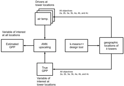
possi-bilities and limitations of the QND tool and validate the results obtained with an example. Figures 1 and 2 show the workflow established for this example. All settings, vari-ables, design questions and the objectives are choices that made it possible to present a relevant example for ongoing discussions within the FLUXNET community. It should be noted that all these aspects of the analysis can be easily adjusted to the needs of the users. At the core of this example is the QND tool based on the k‐means++ clustering algorithm.
[36] This example, which addresses the three design
questions (see 2.1), studied three aspects. The first was the capacity of the existing European eddy covariance tower network (CarboEurope‐IP network) to estimate the gross primary production (GPP or the photosynthetic carbon uptake) of three plant functional types (PFTs): temperate needle‐leaved evergreen (TeNE), boreal needle‐leaved evergreen (BNE), and temperate grassland (TeH). The sec-ond aspect was optimizing the same existing European network for the GPP of TeNE, BNE and TeH. The third was Figure 1. Schematic presentation of how the QND tool was used in the example to obtain geographical
to design an optimal network to sample the GPP of TeNE, BNE and TeH in Europe.
[37] The three design questions were divided into eight
design scenarios, which are shown in Table 2. Scenario 1 corresponds to the current CE‐IP network and, thus, design question 1. Scenarios 2a, 2b, 3a, and 3b correspond to design question 3. In scenarios 2a and 2b, optimal networks are designed with the same number of towers as in the CE‐IP network. In scenarios 3a and 3b, optimal networks are designed with 200 towers. Scenarios 4a, 4b, and 4c corre-spond to design question 2. In addition, four realistic defi-nitions and quantitative objectives for GPP (Table 2) were defined to assess the performance of the proposed networks; that is, monitor the mean, spatial variability, semivariance and spatiotemporal variability of gross primary production (GPP).
[38] Demonstrating some of the possibilities and
limita-tions of the QND tool requires knowledge of the true GPP
for all four quantitative objectives. For this example, in the absence of a map of the true GPP, the target was assumed to be the values simulated with O‐CN, a detailed land surface model (see 2.3.2). O‐CN is used here as a nonlinear and complex transformation of the drivers into the variable of interest (i.e., GPP). The nonlinearity and complexity of this transformation challenges the capacity of the QND tool. Using a model to simulate the true GPP was further justified by the fact that this approach provided full knowledge about the relevant drivers, as the authors were familiar with all the drivers that influenced the simulated GPP. A decision was made to focus on GPP because it has been recently dem-onstrated that it is feasible to upscale starting from point measurements using empirical models [Beer et al., 2010]. This has not yet been demonstrated for net ecosystem exchange (NEE), where disturbances and management play an important role and detailed spatial information of these additional drivers is not yet available.
Table 2. Characteristics of Annual Sums of GPP With O‐CN for Different Design Scenariosa
Scenarios
Annual Sum 2005 Annual Sum 1996–2005b Mean GPP (g C m−2y−1) Spatial Variability of GPP (g C m−2y−1) Semivariance of GPP RMSE of IAV (g C m−2y−1) RMSE (g C m−2y−1) Nugget ((g C)2m−4y−2104) Sill ((g C)2m−4y−2104) Range (km) Baseline, O‐CN 1260 520 9 33 2800 NA NA (1) CE‐IP (42) 1360 ± 90 450 ± 190 11 ± 8 47 ± 105 2900 ± 1200 100 ± 90 410 ± 220 (2a) Opt (42) Clim+N 1230 ± 40 440 ± 20 5 ± 1 20 ± 3 1800 ± 500 60 ± 20 190 ± 40 (2b) Opt (42) GPP 1190 ± 150 520 ± 180 15 ± 15 36 ± 36 2200 ± 1400 120 ± 200 460 ± 320 (3a) Opt Clim+N 1240 ± 20 450 ± 10 6 ± 1 24 ± 2 2600 ± 500 50 ± 10 170 ± 10 (3b) Opt GPP 1100 ± 130 550 ± 90 10 ± 4 38 ± 20 3000 ± 600 100 ± 40 360 ± 70 (4a) CE‐IP+Clim+N 1240 ± 40 470 ± 40 6 ± 4 23 ± 6 1900 ± 900 80 ± 30 220 ± 60 (4b) CE‐IP+Clim 1220 ± 80 500 ± 90 7 ± 3 24 ± 6 1700 ± 700 90 ± 20 260 ± 140 (4c) CE‐IP+GPP 1180 ± 110 560 ± 120 17 ± 12 44 ± 42 2200 ± 1500 100 ± 60 360 ± 110
a
The confidence intervals are computed as 1.96 times the standard deviation of the repetitions used for upscaling.
b
Spatiotemporal variability of GPP on N‐S transect. NA, not applicable.
Figure 2. Schematic presentation of how the ANN was used to upscale the“observation” at the k sam-pling stations proposed by the QND tool.
[39] Depending on the design scenarios of the network
(Table 2), either the drivers (scenarios 2a, 3a, 4a, and 4b) or the variable of interest (scenarios 2b, 3b and 4c) were fed into the design tool (Figure 1). The design tool quantifies cluster centers for k clusters and provides the geographical location of these clusters. The geographical location is selected as the location of the pixel closest to the cluster center in the data space.
[40] The largest reduction in quantization error was used
as the criterion for assigning towers to strata (Table 1, eighth row). The “equal mean quantization error” (Table 1, elev-enth row) was used as the measure of representation in the example and the threshold of representation for using an existing tower was set to 0.5.
[41] At this stage in the workflow, the locations that need
to be sampled are known. For all design questions, the drivers and the variable of interest at these locations are sampled and these data are used to train an Artificial Neural Network (ANN, see 2.3.3). The tower data was not used in this activity, just their location. The trained ANN was then used to upscale GPP to the European domain by making use of the drivers. At this point in the analysis, two spatially explicit maps are available: one of the target GPP and one of the network‐derived GPP. These maps are then post-processed according to 2.3.4.
2.3.2. Obtaining Target GPP Data: The O‐CN Model [42] The O‐CN model [Zaehle and Friend, 2010; Zaehle
et al., 2010] is developed from the land surface scheme ORCHIDEE, described by Krinner et al. [2005], and has been extended by representing the key nitrogen cycle pro-cesses. O‐CN simulates the terrestrial energy, water, carbon, and nitrogen budgets for discrete tiles (i.e., fractions of the grid cell) occupied by up to 12 plant functional types (PFTs) [see Krinner et al., 2005] from diurnal to decadal timescales. The model can be run on any regular grid and is applied here at a spatial resolution of 0.5° × 0.5°. The model has been conceived as a land surface scheme and links a soil‐ vegetation‐atmosphere transfer scheme, dealing with energy and water fluxes [Ducoudré et al., 1993] to representations of short‐ and long‐term carbon cycling [Viovy, 1996] and vegetation structure [Sitch et al., 2003]. The main features of nitrogen dynamics in O‐CN, described in detail by Zaehle and Friend [2010], are (1) prognostic plant tissue N con-centrations, (2) N control on leaf‐level photosynthesis and plant respiration, (3) nutrient status‐dependent allocation to different plant organs, (4) N control on soil organic matter decomposition and N mineralization rate and (5) half‐hourly leaching and gaseous N losses resulting from nitrification and denitrification processes in the soil.
[43] The model setup and results are described in detail by
S. Zaehle et al. (manuscript in preparation). Annual maps of cropland, grassland, primary and secondary forest, and urban areas at 0.5° × 0.5° spatial resolution were obtained from Hurtt et al. [2006] for the period 1700–2005. Coun-trywise total N fertilizer application rates were obtained for 1960–2005 from the FAO statistical database (FAOSTAT accessed in 2009) and spatialized using the yearly cropland extent and an interpolated map of 1995 fertilizer application rates per unit area [Bouwman et al., 2005]. Wet and dry deposition rates of reduced and oxidized Nr for decadal time slices between 1860 and 2000 were obtained from TM3 [Dentener et al., 2006] and linearly interpolated in time to
obtain yearly fields of reactive N deposition. Monthly cli-matologies of air temperature, precipitation, wet days per month, cloudiness, and wind speed were obtained from CRU for 1901–2005 at 0.5° × 0.5° spatial resolution (see Mitchell and Jones [2005] for details). These were dis-aggregated in time to half‐hourly values using the weather generator as in the work by Krinner et al. [2005]. Atmo-spheric CO2concentrations from 1750 to 2005 were used as
in the work by Vetter et al. [2008].
[44] O‐CN was brought to equilibrium with respect to
preindustrial carbon and nitrogen stocks and fluxes using representative forcings of preindustrial conditions of atmo-spheric [CO2] (1750), atmospheric N deposition (1860),
fertilizer applications and land cover (1700). Monthly cli-matologies were drawn annually and randomly from the period 1901–1930. From this equilibrium state, a transient simulation from 1700 to2005 was performed, considering the historical changes in land cover, N fertilizer and N deposition, atmospheric [CO2] and climate. Simulated 0.5° ×
0.5° GPP from the years 1996 to 2005 were used in the example.
2.3.3. Upscaling Using Artificial Neural Networks [45] GPP from tower data to pixel level was upscaled in a
similar manner as Papale and Valentini [2003] and Beer et al. [2010]. A feed‐forward back‐propagation artificial neural network (ANN) was trained using the Levenberg‐Marquardt algorithm [Levenberg, 1944; Marquardt, 1963]. The basic computational unit of the ANN is a neuron, which receives multiple inputs from the previous layer of the network and produces a weighted and nonlinearly transformed output to the next layer. For all tower network evaluations and opti-mizations presented in this study, the climatic variables used as input data of the ANN were air temperature, precipitation, shortwave downward flux, longwave downward flux, spe-cific humidity, N deposition, and N fertilizer. In this study, separate ANNs were trained for the eight scenarios. The data used as input variables of the ANN were a subset of the drivers used in the O‐CN simulations, although the time resolution was different (i.e., daily for O‐CN and annual for the ANN). The hyperbolic tangent sigmoid transfer function was used in the hidden layer of the ANN and the hidden layer contained six neurons. The data was normalized line-arly into zero mean and unit variance for the ANN.
[46] The ANN training makes use of 10 data sets,
com-posed by randomly choosing nine of the 10 years. For each of these 10 training data sets, the ANN is trained by feeding the inputs at the stations with the aim of predicting the target output values from the input values, for which the ANN had never been presented. In order to achieve this goal, the ANN needs to learn from the examples. These examples are the values of the driver variables and the variable of interest at the stations in the 9 years of the training set. The values of the driver variables pass through the ANN and produce an output. This output is then compared with the expected output and the error in prediction is back‐propagated in the ANN to adjust the weights of the neurons in the ANN in order to minimize it and improve the prediction capacity. However, learning should find a balance between overfitting (that is, losing the ability to generalize based on new examples) and overgeneralization. This balance is achieved by selecting a suitable number of neurons in the hidden layer and leaving part of the data for validation. The remaining year
was used to validate the ANN during training. The validation set made it possible to calculate the error of unseen data and prevented overfitting by terminating the training once the error of the validation set no longer improved. For each of the 10 training sets, five networks with different initial connec-tion weights were trained and validated, as described above. From the five ANNs that were trained, the ANN with the lowest error was used for upscaling. This approach was used to prevent using an ANN that reached a poor local minimum during training. In addition, the 10 different ANNs were used to compute the uncertainties of the upscaling results. The trained and validated ANNs were then used to obtain esti-mates of GPP for all grid cells of Europe by feeding the cli-matic variables and N variables into the ANN. In other words, the gridded data was the test set in this study.
2.3.4. Postprocessing
[47] Upscaling with an ANN, as described above, resulted
in a spatially explicit map of the estimated GPP based on data from k sampling locations, as proposed by the QND tool. These maps were postprocessed for four realistic quantitative objectives. The objectives were that the sam-pling network should reproduce the mean GPP, its spatial variability, the spatial structure of the GPP (where the spa-tial structure was defined using the parameters of the semivariogram), and the GPP and its interannual variability along a north‐south transect. For each objective, the target value/variance/distribution was calculated from the O‐CN model output.
[48] For scenarios 1, 4a, 4b, and 4c (Table 2), an existing
network had to be assumed. To this end, the real locations of the eddy covariance towers within the CarboEurope‐IP network were used (Table S1).1This example was limited to three common PFTs: temperate needle‐leaved evergreen (TeNE), boreal needle‐leaved evergreen (BNE), and tem-perate grassland (TeH). No observed data was used at these locations. For internal consistency (see discussion), this example only uses the O‐CN input and output data.
[49] The spatial structure of GPP was determined by
means of the nugget, range, and sill of the semivariograms [Goovaerts, 1997]. Nugget and sill characterize the spatial variation of the data at very small and large distances, respectively. Nugget is defined as the value of semivariance at the shortest‐distance interval (0–100 km) and sill is defined as the maximum value of semivariance. Range is the distance at which semivariance reaches 95 percent of the sill. Because semivariance calculations require stationarity, linear trends with latitude were removed when calculating the semivariance. Less than two percent of all pairwise lags exceeded 3500 km. Hence, lags above 3500 km were not considered in determining the semivariogram parameters.
[50] The ability of the proposed tower networks to
reproduce the spatiotemporal variability of a north‐south transect is quantified using two measures: the root mean squared error (RMSE) of GPP and the RMSE of the inter-annual variability of GPP. The transect is selected as the grid cells centered at longitude 14°75′E. The RMSE of the annual sum between 1996 and 2005 is the root mean squared difference between the upscaled GPP and GPP simulated by O‐CN along the transect. The RMSE of the
interannual variability was calculated as the root mean squared difference between the interannual variability of the upscaled result and simulated GPP along the transect. Interannual variability was calculated for each grid cell as the standard deviation of the GPP value over the 10 year period. In both cases, the upscaled results were compared to O‐CN, which is considered the target value of GPP. Therefore, the RMSE of O‐CN is zero and a small value indicates an upscaling result that agrees with the result of O‐CN.
3.
Results
3.1. Target GPP and Representativeness of the Current Network
[51] The capacity of the current CE‐IP network was
studied first in order to simulate the annual mean gross primary production (GPP), its spatial variability, the struc-ture of the spatial variability and spatiotemporal variability. The target GPP was considered to be the GPP simulated by O‐CN (Table 2). Three plant functional types (PFTs) were studied: Boreal needleleaf forest (12 percent of the pixels under study), temperate needleleaf forest (33 percent) and the temperate humid grassland (55 percent). In Europe, the mean combined GPP for the three plant functional types under study was 1260 g C m−2 y−1; the spatial variability was 520 g C m−2 y−1 and, when characterized by its semivariogram, the nugget was 9 (g C m−2 y−1)2, the sill 33 (g C m−2 y−1)2and the range 2800 km.
[52] When using the true location of 42 existing towers
(Table S1) and the O‐CN input variables, upscaling from the current network would result in an eight percent overestimation of the mean GPP (1360 ± 90 g C m−2y−1) and an underestimation of its spatial variability (450 ± 190 g C m−2 y−1). In addition, when the spatial variability was characterized by its semivariogram, the nugget was 11 ± 8 (g C m−2y−1)2, the sill 47 ± 105 (g C m−2y−1)2and the range 2900 ± 1200 km. The RMSE between the target GPP and the GPP derived from the current sampling network along a north‐south transect is 410 ± 220 g C m−2y−1; the
RMSE of the temporal variability along the same transect is 100 ± 90 g C m−2y−1.
[53] Figure 3 shows the spatially explicit distribution of
GPP derived by upscaling data from the 42 towers. The current network shows a large mismatch (>20 percent of the target GPP) between the upscaled and target GPP, especially on the edges of the European continent. This mismatch is mainly due to gaps in the sampling network (Figure 4). The correlation between the mismatch in GPP and the distance of each grid point from the nearest tower (Figure 5) demon-strates the capacity of the QND tool to detect observational gaps in a network design. The coefficient of determination of the ordinary least squares regression model in Figure 5 is 0.37 and the p value of the model is <0.01.
3.2. Optimizing the Current Network
[54] Across the three PFTs considered in this study, the
flux tower network contains 42 towers or measurement sta-tions. The first step was to quantify how the current network of 42 towers could be optimized without increasing the management costs of the network (Table 2, scenario 2a). Note that this optimization involves two stages: (1) reallocation
1
Auxiliary materials are available in the HTML. doi:10.1029/ 2010JG001562.
of towers across PFTs and (2) relocation of towers within a PFT. Although network 2a, with 42 towers optimized using the drivers, performs slightly better for monitoring the mean GPP, the main gain of this optimization is in the reduction of uncertainty, specifically in the spatiotemporal variability along a N‐S transect, which is captured much better with the optimized network. Also note that the current and optimized networks both performed poorly when the spatial variability was assessed as the standard deviation of annual sums across pixels.
[55] The next step was to assess the improvement in
the network’s performance if 200 measurement stations, a number well above the actual foreseen development of the European network, were allowed (Table 2, scenario 3a). Increasing the number of towers from 42 to 200 results in small improvements of the mean estimates of GPP and further reduces its uncertainty (Table 2). However, estab-lishing 200 towers would still result in an underestimation of the spatial variability. This result is potentially due to placing the towers as close to cluster centers as possible, Figure 3. Relative mismatch of annual sum of GPP in 2005 obtained by upscaling the CE‐IP network.
The shade of gray shows the magnitude of relative error.
Figure 4. Distance to nearest tower of the CE‐IP network in data space. The shades of gray show the tertiles of distances.
which may leave extreme climatic conditions relatively poorly represented, even with a high number of towers.
[56] Finally, the innovative feature of the QND tool was
used to optimize the current network by reusing as many of the current towers as possible (Table 2, scenario 4a). Opti-mization of an existing network requires the user to make a tradeoff between keeping a tower that does not perfectly represent the cluster to which it belongs but which may have considerable time series of data, receive sustainable funding or may be more conveniently located than the optimal tower. This tradeoff was built into the QND tool by setting a threshold of 0.5 for the mean quantization error around a tower in data space (Table 1, eleventh row). Using this approach, 17 of the initial 42 towers passed the threshold and were thus reused. Consequently, 25 new towers had to be established across and within PFTs. As might be expected, the network performance ranks between the current (Table 2, scenario 1) and the optimized (Table 2, scenario 2a) network with 42 towers. Reusing existing towers results in a better estimate of the spatial variability, probably because the reused towers are not the best choice to represent the mean condition of the cluster, but the distance from the cluster center does help to better monitor the variability inside the cluster.
[57] An additional test was performed, in which 25 towers
were added in a manner similar to that in scenario 4a except that all the existing towers were preserved. Preserving all of the existing towers had a minimal effect on the results. This was somewhat expected, given that, even with a network with 200 sites, performances did not improve substantially compared to a network with 42 sites. In principle, however, adding new towers should always produce a better result.
3.3. Drivers Versus Variable of Interest
[58] This study attempted to design the network in such a
way that it is representative of the variable of interest; in this case, GPP. From a design perspective, sampling can be representative in the data space of the variable of interest itself, its main drivers or all its drivers. Using simulated GPP with a process‐based model made the drivers of the target modeled GPP known, which made it possible to test the effect of designing networks that are representative for the variable of interest or its drivers. In general, the performance of the networks that representatively sample the variable of interest (Table 2, scenarios 2b, 3b, and 4c) is poorer than that of networks that representatively sample the drivers of the variable of interest (Table 2, scenarios 2a, 3a, 4a, and 4b). Designing the sampling network in such a way that it represents all drivers (Table 2, scenario 4a) rather than the most important drivers (Table 2, scenario 4b) slightly reduces the uncertainty of the network. Unexpectedly, however, the spatial variability may be slightly better estimated when not all drivers are considered.
3.4. Allocating New Sites to PFTs
[59] In designing an optimal network for different plant
functional types (the same applies for any strata), an essential initial step is for the tool to calculate the order in which stations are allocated to the different strata (vegeta-tion types in this case). Two approaches were implemented (Table 1, eighth row). In the first approach, towers are allocated to the PFT where the largest absolute reduction in the quantization error is achieved (Figure 6, top). The allocation is initialized by assigning one tower to each PFT. Towers 4 to 6 are then assigned to temperate humid grass-lands, towers 7 to 13 are allocated alternately to temperate Figure 5. Relationship between absolute mismatch of annual sum of GPP in 2005 (Figure 4) and
needleleaf forests and humid grasslands, and the rest of the towers are assigned to all three PFTs. When in total 67 towers have been assigned, the boreal needleleaf forest contains 12 percent of the towers, the temperate needleleaf forest contains 39 percent and the temperate humid grassland contains 49 percent. This allocation scheme guarantees that every additional tower maximizes its effect on the network as a whole. However, results from different PFTs can have different uncertainties.
[60] In the second approach, new towers were allocated to
the PFT with the highest absolute quantization error, which reduced the quantization error of that PFT. Again, the allocation is initialized by assigning one tower to each PFT. Towers 4 to 6 are allocated to temperate humid grasslands, towers 7 to 66 are assigned alternately to temperate nee-dleleaf forests and humid grasslands, and only after 66 towers have been allocated to the temperate PFTs does the boreal PFT have its second tower assigned (Figure 6, bottom). At that point in the allocation scheme, three percent of the towers have been allocated to boreal needleleaf forest, 25 percent to temperate needleleaf forest and 72 percent to temperate humid grassland. This allocation scheme
guar-antees that all PFTs are sampled with a similar uncertainty. The average uncertainty, however, is larger in PFTs with a smaller area due to a relatively small number of towers.
4.
Discussion
4.1. Possibilities of the QND Tool
[61] The proposed QND tool can deal with three general
network design questions. (1) How representative is an existing network and in which regions does the network performs poorly? (2) Where should measurement stations be added or removed in order to optimize an existing network? (3) How should a new network of measurement stations be designed so that it is optimized (i.e., contains the minimal number of stations to obtain a specific pre-cision and accuracy for its objectives)?
[62] Although the three design questions are not specific
to monitoring terrestrial ecosystems, our QND differs con-ceptually from the tools used in, for example, ozone moni-toring [Wu et al., 2010] or mobile telecommunication networks [Amaldi et al., 2003]. In the case of ozone moni-toring, the formation and transport of ozone are well under-Figure 6. Relationship between the number of towers and the quantization error. The result corresponds
to scenario 2a (also 3a, quantization error with 200 towers not shown). Solid line shows the results for the temperate needleleaf forest, dashed line shows the boreal needleleaf forest, and dash‐dotted line repre-sents temperate humid grassland. The vertical dotted lines show when the second towers are added to temperate and boreal needleleaf forests. (top) The option of placing the tower to the PFT, which provides the maximum reduction of quantization error. (bottom) The option of placing the tower to the PFT with maximum remaining quantization error.
stood and, therefore, the network can be designed mainly based on urbanity. The network design is governed by esti-mated traffic distribution and physical laws that are reason-able well understood; that is, the power of an antenna or atmospheric transport (and therefore the design tool) relies on a mathematical description of the governing physical laws.
[63] On the contrary, the drivers of the behavior of
ter-restrial ecosystems (soil fertility, soil hydrology, manage-ment and species interactions to manage-mention a few) are poorly understood and are only partly included in mathematical models [Friedlingstein et al., 2006; Hungate et al., 2003]. Consequently, the design tool for a terrestrial carbon exchange monitoring network is not based on a physically known mathematical model but on spatially explicit data related to the variable of interest (note that O‐CN was used to validate the QND tool, not evaluate or optimize repre-sentativeness of the monitoring network). The downside of such an approach is that the outcome of the QND tool cannot be generalized beyond the specific input data used in the representativeness or network design analysis (in the present example, the data produced by the O‐CN model).
[64] The application of the QND tool presented in this
study evaluates eight design scenarios for four objectives (Table 2) by using GPP estimates from O‐CN simulations at tower locations proposed by the tool and by using an ANN for upscaling to other locations. The use of the QND tool is not limited to the practical choices made in this application; the tool can be used to study other design scenarios as long as they relate to evaluating representativeness of an existing network, optimizing an existing network or designing an optimized network from scratch. In addition, any quantita-tive objecquantita-tive, including prediction of the mean, prediction of extremes and observing trends such as GPP, TER and NEP, could be studied by means of the QND tool. Further, the tool does not require the use of models such as O‐CN or ANN, which have only been used for demonstration and validation purpose in this study.
4.2. Flexibility Versus Hidden Assumptions
[65] The QND tool comes with a series of settings (Table 1)
intended to increase flexibility for the users. However, these settings affect the outcome and should therefore be seen as hidden assumptions. Irrespective of which of the three design questions is targeted, the outcome of the study largely depends on the number of strata, as well as on the variable used for stratification and their characteristics in terms of spatial and temporal resolution. Each stratum will at least contain one measurement station and additional sta-tions are assigned to a specific stratum based on its error reduction. The exact criterion used to quantify error reduc-tion may be one of the most important settings of the QND tool because different settings result in a completely dif-ferent number of stations per PFT (see 3.4; Figure 6). Currently, the tool also assumes that the drivers are equally important for all strata. This assumption may not be realistic in all cases, but in the absence of further information, the simplest assumption of equal importance is reasonable. Nevertheless, the QND tools guarantees that strata are re-presented in a rational way. Hence, it is considered more important to fully represent the variable used for stratifica-tion than the other variables used to evaluate or design the network.
[66] In addition, regardless of which of the three design
questions is targeted, network evaluation and design are an unconstrained problem because, in the absence of quanti-tative targets, there is no single solution. For a user willing to accept a large degree of uncertainty, one tower can rep-resent the whole domain, whereas every location needs its own measurement station for users who are not willing to accept any uncertainty in the outcome. If administrative or financial issues limit the number of towers, the network will come with a certain precision. If, however, a precision is put forward, the number of towers is a consequence of the precision requirements. The QND tool can evaluate or optimize a network with any number of stations equal or larger than the number of strata. However, the performance of the network largely depends on the number of measure-ment stations specified by the user.
[67] Optimizing an existing network is more challenging
and relies on several user‐defined thresholds. First, the user must decide which stations are retained in the network, regardless of the cost in terms of representativeness (Table 1, ninth row). Second, the user must set a threshold in order to quantify how representative a station should be for it to be retained. Finally, the user must select a measure of repre-sentativeness. There are a range of possible measures of representativeness, most of which are related to the share of data points within the cluster that are located, in data space, within a specified distance from the cluster center. It is fea-sible to construct measures of representativeness that do not restrict the represented points to be located within the same cluster. This is a subject for future research.
4.3. Drivers Versus Variable of Interest
[68] If the objective of a network is to represent a certain
variable (in this example, GPP), the network can be evaluated or designed using only information of this variable (e.g., GPP data) or by using information of the drivers of this variable rather than the variable itself (e.g., climate and N availability data). The variable of interest is most likely to be a nonlinear function of the drivers and, consequently, both approaches are expected to obtain similar results. However, the example in this study shows that the driver‐based networks outper-form the networks based on the variable of interest.
[69] This paper speculates that this result is due to the
nonlinear relationship between the drivers and the variable of interest. Due to this nonlinearity, different values of the drivers may result in the same value for the variable of interest. Where the clustering algorithm is able to distin-guish different groups when the driver data are used, it is not possible to distinguish different groups when the variable of interest is used. In this example, GPP can be suboptimal due to light, water or nitrogen limitations. A driver‐based net-work will distinguish between the light, water and nitrogen limited regions. However, if the suboptimal GPP happens to have similar values due to different limitations, the QND tool will not distinguish between these regions when GPP is the sole input to the tool.
[70] The selection of the variables that will be fed into the
QND tool is a key step and, consequently, has a strong impact on the results. The input variables should be repre-sentative of the relevant processes (i.e., water stress), drivers (photosynthetic active radiation) and state variables (Leaf N) of the variable of interest. At the same time, the use of
variables that are strongly correlated to each other should be avoided because this would result in overestimating the similarity of different locations (see 2.1).
[71] Although the QND tool is scale‐independent, the
interpretation of its results is not. In the present example, site locations were linked to the input data, assuming that cur-rently established towers with their limited footprints observed the average gridded climate of much larger regions. Hence, the current result cannot be interpreted at the station level because individual stations could experience micro-climates. Therefore, it is even possible that, for example, the Norwegian coastal region is better represented by a station at the west coast of the UK 1000 km away than by a station 100 km inland in Norway. In a representativeness analysis, the use of variables measured at the sites can help to address this aspect; in the network design applications, once the climate characteristics of the representative tower are found, it would be necessary to find sites with a similar microclimate.
4.4. Representing Spatial Variability
[72] Following clustering, the QND tool assumes that if
the cluster must be represented by a single point, the cluster center is most suitable for this purpose. Representing clus-ters by their respective cenclus-ters, in data space, largely ignores the variability within the cluster; hence, the QND tool acts as a smoother. As the current example shows (Table 2), a handful of stations make it possible to represent the mean value of the variable of interest (in our example GPP). However, because the QND acts as a smoother, increasing the number of stations from just over 40 to 200 has only a limited effect on the capacity of the network to capture the spatial variability. It is unlikely that further increasing the number of stations within reasonable limits would overcome this issue because every new station is located as close as possible to the cluster center rather than on the edges of the cluster, which means that it does not represent the extreme values that determine the spatial variability.
[73] In this respect, it is interesting to see that the capacity
of the network to capture the spatial variability is higher when the current network is optimized, as opposed to designing an optimal network from scratch. When opti-mizing an existing network, the user retains established stations, despite the fact that these stations are not as rep-resentative as they could be. In technical terms, suboptimal means that the station is not located in the cluster center. Being away from the cluster center implies that the station better accounts for extreme values within the cluster at the expense of being less representative for the cluster as a whole. Therefore, retaining suboptimal stations improves the capacity of the network to represent the spatial vari-ability within the domain.
[74] The eddy flux network in Europe has been
con-structed in 15 years without following a formal design. One frequent criticism is that the investigators who selected the sites did not account for the representativeness of the sites and paid more attention to the logistical aspects and the usefulness to local and specific scientific questions (such as management effects and carbon sink capacity) or selected ecosystems with a very high or very low productivity. Although this is likely to be true, it may not hamper the usefulness of the network as much as is often suggested. A
network of extremes is likely to represent the mean value but, contrary to an optimally designed network, a network of extremes is more likely to capture the spatial variability of the variable of interest. These important aspects should be considered when the design of a network is started or optimized.
4.5. Future Developments
[75] While working on the above mentioned QND tool, it
became apparent that there was a lack of understanding regarding several critical aspects of network design, often specific to terrestrial ecosystems. Future developments of the tool could be structured along the following lines.
[76] 1. As discussed above, QND acts as a smoother, as the
underlying statistical approaches favor mean‐representative ecosystems rather than ecosystems that operate at the extreme ends of the sampled data space. Consequently, designed networks tend to capture the mean properties of the data space for which they were designed but fail to describe its extremes. As this is a fundamental issue, it is independent of scale and resolution and persists even following data stratification. The tool should be adjusted in such a way that it designs a network of extremes. Several options could be tested, ranging from simply using a new measure of repre-sentation (Table 1, eleventh row) that better accounts for the extremes to a more complex approach in which towers are located in the cluster center when the cluster is surrounded by other clusters and otherwise, the tower is located at the cluster edges. Subsequently, the properties of such a net-work will need to be studied.
[77] 2. The outcome of QND depends on the objective and
data space for which the network has been designed. However, monitoring networks have been operated for a long time. Therefore, there is widespread appreciation of the fact that the research objectives (and therefore the relevant data space) may change during the lifetime of a network in particular for ecosystem networks where the potential uses of the data are very heterogeneous (for example, ongoing FLUXNET synthesis activities address issues in ecophysi-ology, ececophysi-ology, model development, model parameteriza-tion, model validaparameteriza-tion, and upscaling). Some of these activities or changes in research objectives can be antici-pated (such as climate change, land use change, and eco-system vulnerability to extremes in climate) and should be accounted for in the network design. Building on this rationale, the QND tool should be developed so that it can handle multiple objectives and data spaces for studying representativeness of existing networks, designing new networks or optimizing the design of operational networks. [78] 3. QND for large geographical regions, such as
Europe, relies heavily on coarse resolution data. QND suggests the best locations based on coarse resolution data (1–25 km2
) but the research site where the infrastructure will be build represents a much smaller footprint (0.5–1.5 km2
) and does not necessarily represent the coarse resolution pixel characteristics (e.g., climate, vegetation, seasonal trends) accurately. This mismatch in scales is especially clear in, for example, the microclimate of a site in moun-tainous regions or the age of a forest site. Future work should study the limitations and possibilities of high‐resolution variability on coarse resolution QND. For this purpose, the use of site‐level data within a coarse resolution network could