Titre:
Title: Stability of cracked concrete hydraulic structures by nonlinear quasi-static explicit finite element and 3D limit equilibrium methods Auteurs:
Authors: Flavien Vulliet, Mahdi Ben Ftima et Pierre Léger Date: 2017
Référence: Citation:
Vulliet, Flavien, Ben Ftima, Mahdi et Léger, Pierre (2017). Stability of cracked concrete hydraulic structures by nonlinear quasi-static explicit finite element and 3D limit equilibrium methods. Computers & Structures, 184, p. 25-35.
doi:10.1016/j.compstruc.2017.02.007 Document en libre accès dans PolyPublie Open Access document in PolyPublie
URL de PolyPublie:
PolyPublie URL: http://publications.polymtl.ca/2482/
Version: Version finale avant publication / Accepted versionRévisé par les pairs / Refereed Conditions d’utilisation:
Terms of Use: CC BY-NC-ND
Document publié chez l’éditeur commercial Document issued by the commercial publisher
Titre de la revue:
Journal Title: Computers & Structures Maison d’édition:
Publisher: Elsevier URL officiel:
Official URL: https://doi.org/10.1016/j.compstruc.2017.02.007 Mention légale:
Legal notice: In all cases accepted manuscripts should link to the formal publication via its DOI Ce fichier a été téléchargé à partir de PolyPublie,
le dépôt institutionnel de Polytechnique Montréal
This file has been downloaded from PolyPublie, the institutional repository of Polytechnique Montréal
STABILITY OF CRACKED CONCRETE HYDRAULIC STRUCTURES BY
1
NONLINEAR QUASI-STATIC EXPLICIT FINITE ELEMENT AND 3D LIMIT
2
EQUILIBRIUM METHODS
3 4
Flavien Vuillet1, Mahdi Ben Ftima2, Pierre Léger3
5 6
1-Graduate student, Department of Civil, Geological and Mining Engineering, 7
Polytechnique Montréal, Montreal University Campus, P.O. Box 6079, Station CV 8
Montréal, Québec, Canada, H3C 3A7 9
E-mail: flavien.vuillet@polymtl.ca
10 11 12
2-Assistant Professor, Department of Civil, Geological and Mining Engineering, 13
Polytechnique Montréal, Montreal University Campus, P.O. Box 6079, Station CV 14
Montréal, Québec, Canada, H3C 3A7 15
E-mail: mahdi.ben-ftima@polymtl.ca
16 17 18
3-Professor, Department of Civil, Geological and Mining Engineering, 19
Polytechnique Montréal, Montreal University Campus, P.O. Box 6079, Station CV 20
Montréal, Québec, Canada, H3C 3A7 21 E-mail: pierre.leger@polymtl.ca 22 23 24 25 Contact person: 26 27
Professor Mahdi Ben Ftima 28 Phone: (514) 340-4711 ext. 2298 29 Fax: (514) 340-5881 30 Email: mahdi.ben-ftima@polymtl.ca 31 32
Manuscript of a paper submitted for review and possible publication in 33
Computers & Structures 34 35 36 37 Revision 1: January 16, 2016 38
Abstract: Several hydraulic concrete structures suffer from severe tridimensional (3D) discrete 39
cracking, producing an assembly of concrete blocks resting one on top of the other. It is important 40
to consider the 3D particularities of the cracked surfaces in the nonlinear sliding safety evaluation 41
of these structures. A methodology to assess a sliding safety factor (SSF) and a sliding direction D 42
for any structure with an a priori known 3D discrete crack surface geometry using the quasi-static 43
explicit nonlinear finite elements method (QSE-FEM) is presented herein in the context of the 44
strength reduction approach. QSE-FEM is known for its efficiency in solving highly nonlinear 45
problems compared to implicit FEM. However, in QSE-FEM, the determination of the incipient 46
failure motion is challenging. In addition to the ratio of kinetic to internal strain energy, a new 47
criterion is proposed to identify sliding initiation based on absolute displacements of a control 48
point. As part of the proposed methodology, a complementary simple tool, 3D-LEM, has been 49
developed as a 3D extension of the classical limit equilibrium method (LEM). It is useful in 50
preliminary sliding analyses to estimate the critical friction coefficient inducing sliding and the 51
corresponding direction D. Three benchmark examples, of increasing complexities, are presented 52
to verify the performance of the proposed methodology. Finally, a case study is adapted from an 53
existing cracked hydraulic structure to evaluate its sliding stability using the QSE-FEM and 3D-54
LEM approaches. In the three benchmark examples, the same results are found for SSF and D for 55
the two approaches. In the hydraulic structure example, SSFLEM, computed with 3D-LEM, is a 56
lower bound of SSFFEM from QSE-FEM, and a strong correlation is found between the sliding 57
directions computed with the two approaches. 58
Keywords: Finite elements; quasi-static explicit analyses; limit equilibrium; three-dimensional 59
analyses; sliding safety assessment, concrete hydraulic structure 60
1 Introduction 62
Several concrete gravity dams and spillways have been subjected to severe three-dimensional (3D) 63
discrete cracks induced, for example, by concrete expansion due to alkali aggregate reaction 64
(AAR), producing an assembly of unreinforced cracked mass concrete blocks resting one on top 65
of the other (Fig. 1). Discrete cracks of complex non-planar and irregular surface geometries tend 66
to occur and become localised in structures exhibiting geometrical and stiffness discontinuities 67
along their longitudinal axes. As typical examples, the following structures showing this type of 68
damage pattern have been reported in the literature: Beauharnois dam, Canada [1]; Fontana dam, 69
USA [2]; La Tuque dam, Canada 3]; Chambon dam, France [4] and Temple-sur-Lot spillway 70
piers [5, 6]. The definition of the crack surface topology (Figs. 1b and 1c) is possible through site 71
investigation using: (i) visual inspection of crack contour on the downstream face and the exposed 72
pier surfaces; (ii) inspection with a geo-camera installed on a submarine for the upstream face, and 73
(iii) concrete vertical drilling from the dam crest. For this type of cracked concrete hydraulic 74
structure, it is important to consider the 3D particularities of the crack contacting surface 75
geometries in the presence of uplift pressures. The finite element (FE) solution to detect 3D relative 76
crack surface motions of arbitrary geometry, leading to sliding or rotational failure mechanisms, 77
is a highly nonlinear frictional contact problem that is difficult to solve using the classical nonlinear 78
implicit finite element method (FEM). For sliding stability, FEM using a Mohr-Coulomb frictional 79
model can be performed using the strength reduction method in which the friction coefficient is 80
progressively reduced to induce sliding displacements. Strength reduction method has been 81
successively applied in the field of geotechnical engineering for quantifying slope stability. 82
Recently, Tu et al. [7] used FLAC3D to study the stability of 2D and 3D slope problems. Energy 83
based criteria were developed to define the incipient slope failure. The criteria are based on 84
detecting changes in kinetic, potential or strain energy of the model. The results were consistent 85
with the safety factors determined by conventional criteria based on changes in the stresses, strain 86
or displacement distributions in the slope. Though the results were satisfying using the energy 87
criteria, they were applied on simpler problems, if compared to the case study problem shown in 88
Fig. 1. The applicability of Tu et al. [7] methodology based on energy criteria is therefore 89
questionable for the general case where the geometry of the failure surface is arbitrary and where 90
the direction of the sliding is not easily predictable. 91
Constitutive laws for materials can also exhibit highly nonlinear softening behaviour due to alkali– 92
aggregate reaction (AAR) degradation or other structural effects. Convergence difficulties may 93
arise when using the conventional implicit FEM in the context of large concrete models, leading 94
to premature "numerical" failure [8]. Using the explicit FEM approach, the numerical problem is 95
solved dynamically using Newton’s second law of motion. This approach was found to be very 96
efficient for solving highly nonlinear problems such as impact and large displacement problems 97
[9]. The distinct element method (DEM), using an explicit solution algorithm, has been widely 98
used for stability assessment of jointed rock slopes, tunnels and dam foundations 10. DEM 99
commercial software such as UDEC/3DEC recognize individual discontinuities by modelling 100
joints using appropriate distinct (discontinuous) constitutive models from models used for the bulk 101
material. This is in opposition to the classical continuum FEM where the presence of 102
discontinuities in the bulk material has to be represented indirectly in the average sense (i.e. 103
smeared crack models). Lisjack and Grasseli 11 presented a comprehensive review of DEM 104
techniques to assess fracturing of rock masses. Recently, Zhou et al. 12 used ABAQUS/Explicit 105
to develop a combined finite-discrete element method. In their work, a rock mass is idealised as 106
numerous elastic block elements interacting through cohesive joints modeled as contact elements 107
located along their boundaries. Geomechanical problems have been solved at scales ranging from 108
concrete cylinders to slope stability using thousand of discrete elements. The limit equilibrium was 109
reached by increasing the gravitational "constant" (element self-weight) until sliding is detected. 110
The velocity field and the total kinetic energy were used as slope stability indicators. Lately, 111
Abaqus/Explicit models have been applied in the field of concrete hydraulic structures using the 112
quasi-static approach [13, 14]. The nonlinear quasi-static explicit finite element method (QSE-113
FEM) is used in this work as an alternative to the classical implicit FEM. QSE-FEM requires the 114
definition and interpretation of criteria to detect the loss of static equilibrium leading to instability 115
with respect to the initial position. In addition to the kinetic energy criterion used in the previous 116
studies [8, 12, 13, 14], one additional criterion is proposed herein: the absolute crack surface 117
motions at particular degrees of freedom (DOF). In addition, simple tools, such as the classical 118
limit equilibrium method, should be used for verification purposes to bound the sliding safety 119
factors computed from QSE-FEM. For that purpose, a 3D extension of the 2D limit equilibrium 120
method [15], labelled as 3D-LEM, has been developed and implemented in a MATLAB® code as 121
a complementary tool to QSE-FEM. 3D-LEM uses a directional search algorithm to find the 122
minimum sliding safety factor (SSFLEM) and related sliding direction. 3D-LEM is found to be a 123
lower bound solution compared to QSE-FEM. The proposed solution strategies are general and 124
could be applied to any concrete structure with discrete cracks. 125
This paper is organised as follows. First, the QSE-FEM tool is presented. The 3D extension of the 126
classical 2D limit equilibrium algorithm, 3D-LEM, is then developed. An analysis methodology 127
is proposed using QSE-FEM and 3D-LEM as complementary tools. Three validation examples of 128
increasing complexity are investigated to illustrate the particularities of the 3D stability problem. 129
Finally, a case study, adapted from an actual cracked hydraulic structure, as shown in Fig. 1, is 130
analysed showing the performance of QSE-FEM and 3D-LEM. Though applied on an example of 131
hydraulic structure, the framework developed in this study can be applied to a wider range of civil 132
engineering problems where failure may occur through complex and arbitrary 3D surface. 133
134
135
Figure 1: 3D discrete cracking due to AAR expansion: (a) 3D view of hydraulic facility; (b) 136
problematic corner showing 3D discrete cracking; (c) crack mapping on existing structure 137
138
2. Nonlinear quasi-static explicit FEM 139
The explicit dynamics approach was developed and successfully applied in the industrial field of 140
metal forming at the beginning of the nineties [16]. The explicit approach was implemented in 141
several commercial packages (e.g., ABAQUS-Explicit in ABAQUS [9], LS-DYNA [17]). 142
Following an explicit formulation, the nonlinear problem is solved using dynamic equilibrium 143
equations. Conventional nodal forces are converted into inertia forces by assigning lumped masses 144
to nodal DOFs. The dynamic equilibrium equations are written in terms of inertia forces, where M 145
is the lumped mass matrix of the model, P is the external load vector, and I is the internal load 146
vector: 147
𝑴𝒖̈ = 𝑷 − 𝑰 (1)
Compared to the conventional implicit approach, no iteration is performed. The transient solution 148
algorithm advances explicitly in time using a very small time increment to ensure stability. This 149
increment, Δ𝑡, depends on the smallest element of the mesh and can be as low as 10-5 to 10-7
150
fraction of the total analysis time, 𝑡𝑒𝑥𝑝 (Fig. 2). The original nonlinear static problem is solved in
151
a quasi-static manner when the first term in Eq. (1) is negligible. This can be accomplished by 152
applying the loads "slowly enough" with respect to the fundamental period of vibration, 𝑇1, to
153
ensure that kinetic energy, 𝐸𝑘, is negligible compared to the internal strain energy, 𝐸𝑖, [8,9]. As
154
shown in Fig. 2a, a smooth loading time, 𝑡𝐿, is suggested for each load applied separately, such as
155
self-weight, hydrostatic thrusts and uplift pressures, using an established rule of thumb of 20 𝑇1 to
156
50 𝑇1 for the loading time 𝑡𝐿 [8]. This ensures an acceptable evolution of the energy ratio 𝐸𝑘/𝐸𝑖
157
over time as shown in Fig. 2b. Each peak (𝑡𝑖, 𝑟𝑖), 𝑖 > 1, in Fig. 2b represents a typical nonlinear
158
"major event" (e.g., macro-crack propagation in a reinforced concrete beam or local sliding of a 159
surface in a Mohr-Coulomb stability problem). Two important quasi-static criteria must be met 160
for the energy response: (1) considering an energetic criterion, CEng = 𝐸𝑘/𝐸𝑖, the magnitude of
161
CEng at the peaks i for 𝑖 > 1 should be less than 5% (CEng ≤5%); (2) the behaviour of the model 162
shall remain linear elastic within the initial "acceleration" period between 0 and 𝑡0 (Fig. 2b) to
avoid a sudden (dynamic) release of stored elastic energy due to damage. By respecting these two 164
quasi-static criteria, the failure time 𝑡𝑓 of the model is defined as the time where CEng irreversibly
165
exceeds a threshold value (e.g., CEng > 5%). 166
167
Figure 2: QSE-FEM: (a) loading smooth amplitude; (b) typical curve for energy ratio versus time 168
169
In this work, the ABAQUS-Explicit framework is used within the commercial package ABAQUS 170
[9]. The General contact algorithm available in ABAQUS-Explicit is used. It is a robust automatic 171
contact algorithm able to solve complicated and very general 3D contact problems. This contact 172
algorithm has been used extensively in the industry to solve impact tests and automobile crash 173
tests [18]. Using a sophisticated tracking algorithm over the contact domain, the software identifies 174
all node-to-face and edge-to-edge penetrations at each explicit time increment and uses a penalty 175
enforcement of contact constraint in the normal direction. A large displacement sliding method is 176
used in tangential directions, which allows for arbitrary separation, sliding and rotation of surfaces 177
in contact. In the tangential (sliding) direction, displacement continuity is exactly enforced during 178
the stick condition. The sliding constitutive model in the tangential direction neglects the related 179
crack dilation motions in the normal direction due to the interface crack roughness. The dilation 180
effect of concrete-concrete sliding interfaces is implicitly considered in the selected initial friction 181
coefficient according to test data 19 and dam safety guidelines. For the strength reduction method 182
used in this study, a user subroutine, called VFRIC, was programmed to model a user-defined 183
tangential strength, which allows for a progressive decrease in the friction coefficient over time 184
𝜇𝑖(𝑡). The typical variation of 𝜇𝑖(𝑡) is shown in Fig. 3a. The 𝑡𝑗 and 𝜇𝑖(𝑡𝑗) values are user inputs
185
to the subroutine required to compute a continuous curve with smooth interpolation (cubic 186
polynomial) between successive time points. The Mohr-Coulomb criterion is used for sliding with 187
zero cohesion. All computations are performed with static friction coefficients in contrast to using 188
static and dynamic friction coefficients. The first value 𝜇𝑖0 is the initial value of the friction
189
coefficient, constant for the first loading step, which is a local material property for the "ith"
190
discretized FE contact surface. Of course, these friction coefficients must be larger than the critical 191
friction coefficient value that induce sliding. 192
194
195
Figure 3: Procedure used in strength reduction method: (a) variable friction in the tracking 196
phase; (b) sliding interval tracking; (c) constant friction and variable friction analyses in the
197
verification/refinement phases (regular/bold lines); (d) energy ratio evolution in the tracking
198
phase; (e) energy ratio evolution in the verification/refinement phases (regular/bold lines)
199 200 201
In addition to the energy criterion, CEng, a displacement criterion, CDisp, is defined herein. CDisp is 202
related to the absolute displacement magnitude of a selected control point from the upper sliding 203
block. Due to the relatively large magnitude of the sliding displacement with respect to the elastic 204
displacement induced by the deformations of the upper and lower blocks and to the large sliding 205
velocity that is initiated by a sliding failure, it was found that using the absolute displacement is 206
precise enough to detect the onset of the instability (sliding) phase. The control point is a point 207
belonging to the upper sliding surface. It is located at the extremity of the last resisting elements 208
with respect to the sliding direction, D. An example of a control point is presented in the third 209
example of section 5 (Fig. 9). In a more general 3D problem, the selection of the control point and 210
sliding direction is not easily predictable. 3D-LEM is thus introduced in section 3 as a preliminary 211
predictive tool to complement the QSE-FEM analysis. The strength reduction factor SRF(t) is 212
introduced as the ratio between initial and reduced friction coefficients: SRF(t) = µi0 / µi(t) (Fig. 213
3a). Using the CEng and CDisp criteria, the SRF that induces sliding is identified. SSFFEM is defined 214
as the last value of SRF where a stable condition is maintained. 215
216
3 3D Extension of limit equilibrium method 217
3.1 2D limit equilibrium method 218
The bi-dimensional limit equilibrium method (2D-LEM) was documented by the US Army Corps 219
of Engineers in 1981 [20]. The method defines SSFLEM: 220
𝑆𝑆𝐹𝐿𝐸𝑀 =
𝜏𝑎
𝜏 (2)
where 𝜏𝑎 is the admissible shear stress, and 𝜏 is the shear stress on the failure plane. The admissible
221
shear stress is ruled by the Mohr–Coulomb equation: 222
𝜏𝑎 = 𝑐 + 𝜎 ∗ tan (𝜙) (3)
where 𝑐 is the cohesion, 𝜎 is the normal pressure to the failure plane, and 𝜙 is the friction angle. 223
SSFLEM in Eq. (2) can be applied only on a single wedge with a straight cracked plane. An algorithm 224
was thus developed to solve the multi-wedge problem associated with a segmented cracked surface 225
(Fig. 4a). Each segment of the cracked surface defines a wedge by vertical delimitation to each 226
extremity of the segment. Horizontal thrusts, Pi-1 and Pi, are introduced on the left and right sides
of each wedge to equilibrate the shear stress on its bottom segment (Fig. 4b). The force difference, 228 𝑷𝒊−𝟏− 𝑷𝒊, is computed as follows: 229 𝑷𝒊−𝟏− 𝑷𝒊 =((𝑾𝒊+𝑽𝒊)∗cos(𝛼𝑖)−𝑼𝒊) tan(𝜙𝑖) 𝑆𝑆𝐹𝐿𝐸𝑀−(𝑾𝒊+𝑽𝒊)∗sin(𝛼𝑖)+𝑆𝑆𝐹𝐿𝐸𝑀𝑐𝑖 ∗𝐿𝑖
cos(𝛼𝑖)+sin(𝛼𝑖)∗𝑆𝑆𝐹𝐿𝐸𝑀tan(𝜙𝑖)
(4)
where Wi is the weight of the wedge, Vi is the weight of the water above, Ui is the uplift, Li is the
230
length of the ith segment, and 𝛂
𝐢 is the angle between this segment and the horizontal. The SSFLEM 231
corresponding to the sliding limit equilibrium is computed such that the summation of all 𝑷𝒊−𝟏−
232
𝑷𝒊is nearly zero. Moment equilibrium is not satisfied. Therefore, only a global equilibrium of 233
driving versus resisting sliding forces is satisfied along a unique kinematic admissible sliding 234
direction, D, which is horizontal for the case in Fig. 4. 235
236
237
Figure 4: 2D limit equilibrium method; (a) three wedges example; (b) loads on a single wedge 238
239
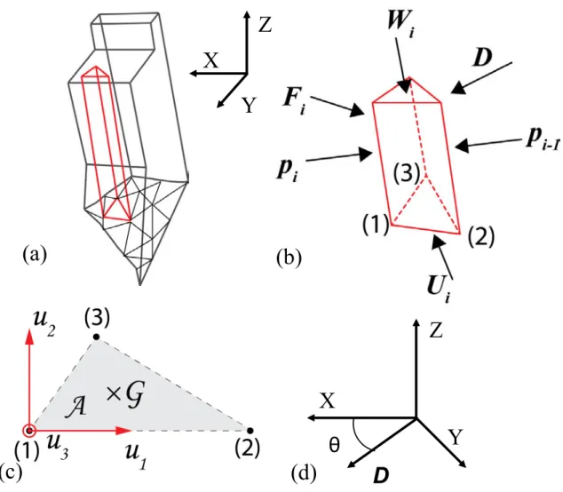
3.2 3D extension of limit equilibrium method 240
The 3D limit equilibrium method (3D-LEM) is defined as an extension of the classical 2D-LEM 241
presented in section 3.1. Fig. 5a presents part of a gravity dam (or an arbitrary concrete structure) 242
with a nonplanar crack pattern at its base. The complete cracked surface is discretized by several 243
elementary triangular surfaces. The volume of the complete structure is divided into adjacent 244
vertical elementary elements labelled as "columns" located between a particular triangle at the 245
cracked surface and the top of the structure. Each column denoted by the index "i", and its related 246
base triangular surface described by nodes 1-2-3, is subjected to several forces: the self-weight, 247
Wi, the uplift pressures, Ui, an arbitrary resultant of external forces, Fi, and the forces Pi and Pi-1
248
associated with the LEM, which equilibrate the shear strain on the base of the column (Fig. 5b). 249
The self-weight of a column, Wi, is defined by the product of material density and the column
250
volume computed from the known geometry. Water pressures are associated with each corner of 251
the base triangle. The average value defines the elementary uplift pressure that is multiplied by the 252
base triangular surface to obtain the uplift force, Ui. The external thrust Fi, could be null or could
253
be the resultant of hydrostatic pressure as an example. 254
256
Figure 5: Definition of 3D-LEM (a) cracked surface divided into triangles and concrete block 257
divided into columns; (b) loads applied on a column; (c) local axis definition for the triangular 258
base; (d) definition of θ and the sliding direction D 259
260
The elementary unbalanced horizontal forces, 𝑷𝒊−𝟏− 𝑷𝒊 or P, are to be computed for each
261
column, following a given direction D. The limit equilibrium condition of the surface along the 262
direction D gives the following equation: 263 𝑐 ∗ 𝐴 𝑆𝑆𝐹 − (𝑾 + 𝑼 + 𝑭 + 𝜟𝑷). 𝒖𝟑∗ tan(𝛷) 𝑆𝑆𝐹 = (𝑭 + 𝑾 + 𝜟𝑷). 𝑫′ ||𝑫′|| (5)
(a)
(b)
(c)
(d)
Z
X
Y
Z
X
Y
D
θ
where 264
𝑫′ = 𝑫 − (𝒖
𝟑. 𝑫)𝒖𝟑 (6)
(𝒖𝟏 𝒖𝟐 𝒖𝟑) defines a local axis system linked to the triangular column base (Fig. 5c). The
265
parameter 𝒖𝟏 is a normalised vector from node 1 to node 2 of the triangle, and 𝒖𝟑 is normal to the
266
triangle and oriented such that the scalar product 𝒖𝟑. 𝒁 ≥ 𝟎. The vector 𝒖𝟐= 𝒖𝟑^𝒖𝟏 is
267
complementary and located in the plane of the triangle. The interface properties introduced in Eqs. 268
(2) and (3) for failure planes in the conventional 2D-LEM are assumed constant for each triangular 269
element at the interface cracked surface and are defined as local material properties for the "ith"
270
discretized FE contact surface. The Mohr-Coulomb equation rules the contact between surfaces, 271
such that a friction coefficient, 𝜇𝑖𝑐𝑟𝑎𝑐𝑘 = tan (𝛷) and a cohesion, ci, are associated with the “ith” 272
contact surface. 273
274
𝑷𝒊−𝟏− 𝑷𝒊 is defined along this same direction D: 275
𝜟𝑷 = 𝑷𝒊− 𝑷𝒊−𝟏= 𝑃 ∗ 𝑫 (7)
The direction D is horizontal and is defined by the angle θ (Fig. 5d). It is assumed that the strength 276
is developed in direction D such that the resisting forces associated with the cohesion and the 277
friction are also along this direction. A vector 𝜟𝑷 is computed for each column. 278
Similar to the 2D-LEM method, the SSF(D) is determined when ∑𝑖𝜟𝑷𝑖= 0. Newton’s method is
279
used to find the "zero" of the summation, which has the advantages of simplicity and quadratic 280
convergence. SSF(D) is computed for each direction 𝑫, and the minimum is identified as SSFLEM 281
related to the corresponding sliding direction, DLEM.
The convergence tolerance to satisfy the equation ∑𝑖𝜟𝑷𝑖 0 has a strong influence on the SSFLEM 283
results. Fig. 6 illustrates several curves drawn for different tolerances where ∑𝑖𝜟𝑷𝑖= 10-1 to 10-4.
284
A "small" tolerance is required for smooth response curves. A real improvement occurs for 285
tolerances smaller than or equal than 10-3; a 10-3 tolerance value is thus used later in the application
286
examples. 287
288
289
Figure 6: Influence of the tolerance on SSF(D) (example 2 considered); (a) tolerance=10-1; (b)
290
tolerance=10-2; (c) tolerance=10-3, D
LEM=D (θ=30.67deg); (d) tolerance=10-4
291 292 293
Eq. (4) could become ill conditioned if the denominator is close to zero. Ebeling et al. [15] 294
suggested that the denominator in Eq. (4) should not be less than 0.2. In 3D-LEM, the ill condition 295
problem is solved by slightly modifying the inclination of the base triangle of problematic 296
columns. The inclination is reduced so that the normal to the base becomes closer to the vertical 297
axis Z. This operation locally modifies the geometry of the cracked surface, but it is acceptable in 298
practice for a structure such as that shown in Fig. 1 because uncertainty always remains on the 299
exact geometry of the crack surfaces. 300
4 Proposed methodology for sliding safety assessment 301
A progressive assessment methodology is suggested in this work, based on the experienced gained 302
through the several numerical studies conducted. 3D-LEM is found to be a simple tool compared 303
to QSE-FEM, giving a lower bound value of SSFFEM. QSE-FEM is a sophisticated FE tool that 304
considers all types of potential unstable conditions by computation of the incipient kinematic 305
motions of all cracked components in the model. It is therefore relevant to any general 3D stability 306
problem: rigid/deformable bodies, linear/nonlinear constitutive material, small/large 307
displacements, imposed displacements/forces, sliding/overturning/uplifting or any combination of 308
these relative motions. As with any sophisticated tool, using QSE-FEM represents challenges in 309
terms of problem sensitivity and abundance of results. The analysis should thus be performed as 310
follows: 311
a) Discretization of the geometry: discretization into triangles of the 3D discrete cracked 312
surfaces in 3D-LEM and 3D discretization with solid elements in the FE model used in 313
QSE-FEM. For consistency, the discrete cracked surfaces are generated with ABAQUS 314
and used as input to MATLAB®. 315
b) Selection of time integration parameters: Compute the stable time increment Δ𝑡 for the 316
QSE-FEM generated mesh. Compute the modal frequencies of the FE model by imposing 317
the full compatibility condition in the interfaces between all cracked components (or 318
wedges) of the model (TIED condition) and fixity condition at the bottom face of the 319
foundation block. Define accordingly 𝑡𝑒𝑥𝑝 for the analysis duration and 𝑡𝐿 for each load
320
condition. Proceed with preliminary analyses using QSE-FEM (only with an initial loading 321
step, 𝑡𝐿) to check the quasi-static criteria.
322
c) Directional search: Proceed with a directional search with 3D-LEM to find SSFLEM and 323
DLEM.
324
d) Initialisation of QSE-FEM: Use the results of step c) to select an initial value of the friction 325
coefficient 𝜇𝑖0 and a control point to monitor the onset of the sliding (criterion CDisp).
326
e) Perform strength reduction: Move forward with a strength reduction step in QSE-FEM 327
within a first tracking phase (Figs 3a, b and d). Identify a sliding interval range using a 328
lower bound and an upper bound, [𝜇𝑖(𝑡𝑙𝑜𝑤), 𝜇𝑖(𝑡𝑢𝑝)], for 𝜇𝑖𝑐𝑟𝑖𝑡 (criteria CEng and CDisp are
329
considered; only CEng is shown in Fig. 3d). 330
f) Verification and refinement to compute μicrit: In this step, three different analyses are 331
considered as shown in Fig. 3c. For verification of the sliding interval range, two analyses 332
with constant friction coefficients are conducted. The values of the friction coefficients are 333
selected to be slightly outside the sliding interval range (an 𝜀 value of 0.05 to 0.1 is to be 334
used). It may happen that, contrary to what is shown in Fig. 3e, the criterion CEng for the 335
case 𝜇𝑖(𝑡𝑢𝑝). (1 − 𝜖) decreases after t0 and follows a tendency similar to the case
336
𝜇𝑖(𝑡𝑙𝑜𝑤). (1 + 𝜖). The reason for this behaviour is the presence of residual inertia forces 337
for each smooth step delimited by 𝑡 and 𝑡 . This behaviour is schematically shown in 338
Fig. 3d at the end of the interval [𝑡0, 𝑡1]. It is necessary for this particular case to return to
339
the tracking phase and set up new bounds of the sliding interval. The increase in the interval 340
length (e.g., the interval [𝑡0, 𝑡1] for the case depicted in Fig. 3) was found to be an efficient
341
solution to reduce the magnitude of the inertia forces. The next step is the refinement of 342
the 𝜇𝑖𝑐𝑟𝑖𝑡 interval range. An analysis with a variable friction coefficient is therefore used
343
(Figs. 3c and e). Similar to the tracking phase, a first initial loading step with constant 344
friction coefficient 𝜇𝑖(𝑡𝑙𝑜𝑤) is followed by a strength reduction step with friction
345
coefficient smoothly decreasing from 𝜇𝑖(𝑡𝑙𝑜𝑤) to 𝜇𝑖(𝑡𝑢𝑝) (Figs. 3c and e).
346
g) Computation of SSFFEM: Estimate the value of the critical friction coefficient, 𝜇𝑖𝑐𝑟𝑖𝑡, the
347
corresponding 𝑆𝑆𝐹𝐹𝐸𝑀 = 𝜇𝑖𝜇𝑖𝑐𝑟𝑎𝑐𝑘
𝑐𝑟𝑖𝑡 and the corresponding sliding direction, DFEM.
348
Complementary analyses could be performed in step f) Verification and refinement to compute 349
μicrit using implicit FEM on the two analyses with constant friction coefficients. If both analyses 350
with constant friction coefficients 𝜇𝑖(𝑡𝑙𝑜𝑤) and 𝜇𝑖(𝑡𝑢𝑝) converge, the interval range
351
[𝜇𝑖(𝑡𝑙𝑜𝑤), 𝜇𝑖(𝑡𝑢𝑝)] is incorrect. The analysis using the coefficient value 𝜇𝑖(𝑡𝑢𝑝) should not lead to
352
an equilibrium state. The methodology then must be initiated again in step e). In any other case, 353
one analysis or both analyses fail such that no conclusion can be deduced due to the possibility of 354
a “numerical” failure of the implicit analyses. 355
5 Validation examples 356
Three validation examples are considered in this section. They represent important issues related 357
to the real case study problem introduced in Fig. 1b. Sliding on an arbitrary inclined plane and 358
tracking of the critical sliding direction are considered in example 1. The problem of locally large 359
uplift pressure with respect to gravity loads, which may occur in the downstream inclined face of 360
a dam (Fig. 1b), is considered in example 2. The multiple-wedge issue is considered in example 3, 361
taken from [20]. In addition to [20], example 1 and example 2 can be considered as new benchmark 362
unit problems that can be used for the verification and validation purposes (V&V) of the stability
363
assessment tool of a general 3D problem. 364
Example 1 – 3D sliding block on an inclined surface 365
This first example illustrates a 3D stability problem of a single massless block sliding on an 366
arbitrary inclined surface (Fig. 7a). Two external driving forces are applied, 5 kN along the Z-axis 367
and 1 kN along the X-axis (Fig. 7b). A sliding analysis direction is required to compute SSFLEM. 368
This direction is projected in the XY plane and is characterized by a directional angle θ defined 369
from the X-axis (Fig. 7d). Sets of SSF(D(θ)) results are computed for series friction coefficients, 370
µ, and for a range of θ (Fig. 7c). The curve tangent to a SSF(D) = 1 defines the minimal friction
371
coefficient for limit equilibrium, which is equal to 𝜇𝐿𝐸𝑀 = 0.435. SSF(D) increases with increasing
372
friction coefficient regardless of the potential sliding direction D. Minimum SSF(D), SFFLEM, is 373
always reached at the directional angle θLEM = 30.67°, irrespective of the friction coefficient. The
374
red point in Fig. 7c indicates 𝜇𝐹𝐸𝑀 = 0.437 computed using QSE-FEM. The sliding motion
375
projected in the XY plane is shown in Fig. 7d. It is a rectilinear motion with a 29.33° directional 376
angle between the X-axis and the sliding direction. 𝜇𝐹𝐸𝑀 = 0.437 develops the frictional strength
377
just able to maintain equilibrium (incipient sliding motion), which has less than 1% difference with 378
𝜇𝐿𝐸𝑀. These nearly identical results between 𝜇𝐿𝐸𝑀 and 𝜇𝐹𝐸𝑀 validate the two stability analysis
379
tools used to characterize the limit friction coefficient and the incipient sliding direction for this 380
basic 3D sliding problem. 381
383
Figure 7: Example 1 of a sliding block on an inclined plane (a) geometry definition of the 384
inclined surface (b) geometry definition of the block, definition of the loads and ABAQUS 385
meshing; (c) SSF computed for three friction coefficients from 3D-LEM and SSFFEM from QSE-386
FEM; (d) sliding trajectory in XY plan of the block with ABAQUS 387
388
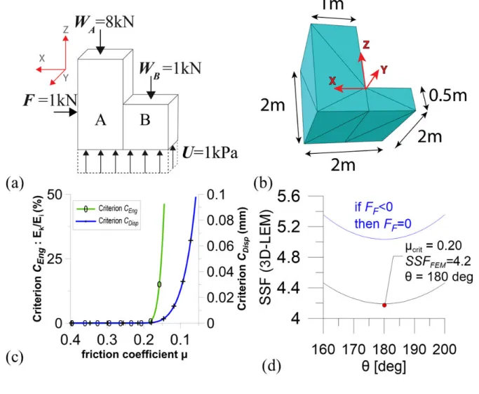
Example 2 – Column with locally large uplift pressures 389
The second example is used to illustrate the effect of vertical uplift pressures locally larger than 390
the self-weight of column B of the structure shown in Fig. 8a. Eq. (5) includes the friction force 391
expression FF = (𝑾 + 𝑼 + 𝑭 + 𝜟𝑷). 𝒖𝟑∗tan(𝛷)𝑆𝑆𝐹 regardless of its sign. It is possible to obtain a
negative FF value if there is a tensile normal force along 𝒖𝟑. In this case, FF has no physical 393
meaning. Considering a structure made of two tied columns A and B (Fig. 8a), the loads are the 394
self-weights WA =8 kN and WB =1 kN for A and B respectively; the uplift pressure U=1 kPa and
395
a horizontal external thrust F=1 kN. The friction coefficient 𝜇𝑐𝑟𝑎𝑐𝑘 equals 0.84 between the
396
structure and the foundation. The uplifting force locally under B (2 kN), is larger than the self-397
weight (WB =1 kN), making this column intuitively “floating” if considered as a free-standing
398
element, even if the complete structure A-B is stable. In that case, using independent free-body 399
diagrams for A and B, no friction can occur between column B and the foundation because there 400
should be no contact. Thus, the expression FF = (𝑾 + 𝑼 + 𝑭 + 𝜟𝑷). 𝒖𝟑∗tan(𝛷)𝑆𝑆𝐹 equals 0 for
401
column B. To test whether we should neglect FF in the case of “floating” columns, two analyses 402
were performed with 3D-LEM: The first with Eq. (5) and the second with a procedure added to 403
neglect FF when its sign is negative. Fig. 8d illustrates the response obtained with Eq. (5) (lowest 404
curve) and the modified equation, which neglect FF for column B (highest curve). The red point 405
in Fig. 8d represents the result computed from QSE-FEM. The correlation between the lowest 406
curve and the red point in Fig. 8d and the analytical solution, which is 𝜇𝑐𝑟𝑖𝑡=0.2 (𝜇𝑐𝑟𝑖𝑡=F(1kN) /
407
[WA(8kN) + WB (1kN) – U(4kN)] = 0.2), demonstrates that the analysis using Eq. (5) directly is
408
correct. Neglecting FF for “floating” columns changes the quantity 𝜟𝑷𝒊= 𝑷𝒊− 𝑷𝒊−𝟏. 𝜟𝑷𝒊 that
409
symbolizes the available resistive strength of the ith column. It is thus important to not modify Eq.
410
(5) because to neglect the negative value of FF is similar to not considering “weak” columns (such 411
as column B) and overestimating SSFLEM. 412
414
Figure 8: Example 2 with locally large uplift pressures (a) loads applied; (b) geometry of the 415
problem and ABAQUS meshing; (c) criteria of QSE-FEM; (d) SSF(θ) according to different 416
considerations on FF value, and QSE-FEM result 417
418
Example 3- Extruded 2D gravity dam – Multi-wedge analysis 419
The example seeks to compute the sliding safety factor (SSFLEM; SSFFEM ) of a 2D 12 m high 420
gravity dam resting on a rock foundation (Fig. 9). This problem has been solved, with detailed 421
calculations, by the standard 2D LEM using a multi-wedge analysis [15, 20, 21, 22]. A non-planar 422
failure surface is formed within the soil and rock foundation and along the dam-foundation 423
interface. The dam-foundation system is divided into 5 adjacent wedges. There are two driving 424
soil wedges, one structural wedge, and two resisting soil wedges. The loads acting on each wedge 425
i are the wedge weight, Wi, uplift pressures Ui, hydrostatic pressure Hi, and vertical water weight
426
Vi. As in the original reference [20], and to be able to draw meaningful comparisons, the uplift
427
pressures are kept constant during the strength reduction process. 428
429
Figure 9: Example 3 of hydraulic structure presented in [20] (a) multi-wedge 2D problem; (b) 430
ABAQUS mesh; (c) wedge displacements of the contact problem (scale: 10/1); (d) wedge 431
displacements of the tied problem (scale: 10/1) 432
Despite its apparent simplicity, this problem is particularly challenging due to the following issues: 434
(1) The presence of sharp contact edges at the intersection of the wedges and sensitivity of the 435
General contact algorithm to this condition; (2) The effect of shear and moment transfer along the 436
vertical interfaces between the wedges; (3) The driving force in the problem that is the hydrostatic 437
force H acting on the upstream face of the dam or wedge 3. This force is exerted on the third wedge 438
element (and not the first) in the wedge chain and results in tensile stresses between the second 439
and third wedges and an overturning tendency of the dam. (4) The abutment effect developed due 440
to resisting soil wedges. 441
Clearly, most of these issues are outside the 3D-LEM tool application range. QSE-FEM can be 442
used to study each issue separately, but this is also outside the scope of this paper. The effect of 443
sharp contact edges has been studied, and no significant effect was found in SSFFEM or in the final 444
instability mechanism. The effect of vertical interfaces between wedges was tested using two 445
conditions: a contact condition with no friction and a full compatibility (or tied) condition. The 446
results of the QSE-FEM are dependent on these conditions and are listed in Table 1 by QSE-FEM-447
contact and QSE-FEM-tied for contact and tied conditions, respectively. 448
449
Table 1: Example 3: Extruded 2D Gravity Dam 450 USACE 2005 SSFLEM 3D-LEM SSFLEM QSE-FEM-contact SSFFEM QSE-FEM-tied SSFFEM 2.0 1.96 2.1 ˃ 8.0 451
One of the advantages of the explicit solution tool in ABAQUS compared to the standard implicit 452
resolution is the way contacts on interfaces are managed, especially how contact between two 453
coincident nodes from a wedge and the foundation is modelled. In the standard implicit tool, the 454
tangential contact before sliding is represented by a penalty coefficient. This allows displacements 455
named “elastic slip”, even if the shear stress is below the allowable frictional shear strength 456
described by Mohr–Coulomb equation. Another alternative for the implicit solution (ABAQUS-457
Standard) is to use the Lagrange multiplier method to enforce exactly the kinematic tangential 458
sticking constraints of the potentially sliding interfaces. This solution tends however to increase 459
the complexity of the problem and convergence issues may arise ([9]). Fig. 10 represents several 460
displacement responses in the tied conditions for constant friction coefficients reduced by a factor 461
of 2 from the initial values. In the implicit analyses, the tangential penalty coefficient is increased 462
systematically to study convergence properties. The implicit solutions are converging to the 463
explicit solution while the penalty coefficient is increasing. QSE-FEM uses the equivalent of an 464
infinite tangential penalty coefficient, which reduces the “elastic slip” to zero. This makes the 465
explicit solution much more efficient than the standard implicit one to detect sliding motions. 466
467 468
469
Figure 10: Absolute displacements of the control point. Convergence of the standard implicit 470
solutions towards the explicit solution when stiffness is increasing. Computed on tied example 3 471
SSF=2
472 473
A good correlation is found for SSF, between [20], 3D-LEM and QSE-FEM-contact conditions. 474
QSE-FEM-tied resulted in a large value of SSFFEM, which can be attributed to the abutment effect 475
of resisting soil wedges. Fig. 11 presents the evolution of the computed SSFFEM versus the 476
horizontal displacement of the control point. A similar tendency has been reported by Wei et al. 477
[23] and demonstrates the obvious dependency of SSF on the displacement of the control point 478
(equal to sliding for infinitely rigid blocks). The problem therefore becomes an engineering 479
problem to decide on the threshold displacement (or sliding) value and compute the corresponding
480
SSF according to Fig. 11.
482
483
Figure 11: Horizontal displacements of the control point for untied example 3 484
485
6 Spillway analysed 486
This section presents the sliding stability analysis of a concrete hydraulic structure adapted from 487
an existing spillway suffering from AAR as shown in Fig. 1. 488
6.1 Description 489
The AAR swelling displacements induced severe cracking at the base end of the gravity dam and 490
the spillway pier adjacent to it (Fig. 1b). The crack and the top of the hydraulic structure separate 491
the extremities of the concrete block. Water flow is visible on the downstream face of the gravity 492
dam (Fig. 1c). The crack is thus going from the upstream to the downstream face. The upper block 493
is considered independent of the rest of the structure and is free to move in any direction. In the 494
existing structure, passive steel anchors have been added to improve the sliding safety. These 495
anchors have not been considered in this application. 496
The material and crack interface properties of this block are displayed in Table 2. Four load 497
conditions are considered: the weight due to gravity (G), the horizontal hydrostatic pressure (H), 498
the horizontal gate thrust (V) on the left of the pier and the uplift pressures (U). Thus, we define 499
one load combination including all load conditions: GHVU. In the context of this application 500
example, we exclude any consideration of AAR effects. 501
502
Table 2: Material Properties 503
Material properties
ρ (kg/m3) Density 2 400
E (MPa) Young modulus 25 000
ν Poisson coefficient 0.2
µcrack Friction coefficient 1.13
C (kN/m2) cohesion 0.0
504
The hydrostatic loads and uplift pressures are defined according to the following outlines: (1) the 505
hydrostatic pressure is maximal upstream of the gate and (2) it linearly decreases downstream of 506
the gate until reaching atmospheric pressure at the downstream face of the gravity dam (Fig. 12). 507
The maximal pressure is defined as the water column height from the crest of the pier and the dam. 508
For simplicity, the uplift pressure diagram was kept constant during the strength reduction process. 509
The gate thrust is produced by the horizontal hydrostatic pressure acting on the gate adjacent to 510
the pier. The gate is 15 m long, and the half-force resultant of this pressure is transmitted to the 511
pier. 512
514
Figure 12: Load conditions on the concrete wedge: H Hydrostatic pressure, U Uplift and V Gate 515
thrust : (a) elevation view; (b) plan view 516
517
6.2 Stability assessment 518
The friction coefficient of the concrete/concrete cracked interface is 𝜇𝑐𝑟𝑎𝑐𝑘 = 1.13. Table 3
519
displays SSFLEM and SSFFEM and the related sliding directions D for the load combination GHVU. 520
Table 3: Comparative results for the GHVU load combination 521 3D-LEM QSE-FEM SSFLEM DLEM θ (deg) SSFFEM Criterion CEng SSFFEM Criterion CDisp DFEM θ (deg) 1.66 106 1.94 1.78 105 522
In the load combination GHVU, SSFLEM = 1.66 is the lower bound in regard to SSFFEM computed 523
with the criteria CEng (SSFFEM = 1.94) and CDisp (SSFFEM = 1.78). The sliding direction θLEM = 106
524
deg is very close to θFEM = 105 deg.
525
The ABAQUS mesh is used for QSE-FEM analyses, and the two convergence criteria for a friction 526
coefficient interval range of [1.13; 0.2] are shown in Fig. 13. According to Fig. 13b, 𝜇𝑐𝑟𝑖𝑡, the
527
critical friction coefficient inducing sliding, lies between 0.7 and 0.4. The methodology described 528
in section 4 was thus applied to reduce uncertainty on 𝜇𝑐𝑟𝑖𝑡. The main observations led to steps a)
529
to g) as follows. Step a: the crack surface geometry was modelled in ABAQUS only according to 530
the onsite measurement of the crack rim, so uncertainty remains in the exact crack surface 531
geometry. Linear tetrahedral FEs were used. Different mesh sizes were tested during the analyses, 532
and no significant influence on SSFFEM or SSFLEM was found. Step d: based on θLEM = 106 deg
533
computed in step c, the monitoring node was defined as shown in Fig. 13a. SSFFEM equals 1.66, 534
corresponding to 𝜇𝐿𝐸𝑀 = 0.683. Thus, the initial value of the friction coefficient for QSE-FEM was
535
set up to 𝜇0=0.7. Step e: the first interval range computed for 𝜇𝑐𝑟𝑖𝑡 was [𝜇(𝑡𝑙𝑜𝑤) = 0.7, 𝜇(𝑡𝑢𝑝) =
536
0.45]. The two verification analyses were performed with 𝜖 = 5% and validated the interval range. 537
Another analysis with the reduced interval range [𝜇(𝑡𝑙𝑜𝑤) = 0.65, 𝜇(𝑡𝑢𝑝) = 0.5] was then
538
performed, and two new verification analyses (𝜖 = 5%) validated the new interval. Step g: using 539
the two criteria CDisp and CEng, the friction coefficients were found: 𝜇𝑐𝑟𝑖𝑡(𝐶𝐷𝑖𝑠𝑝) = 0.637 and
540
𝜇𝑐𝑟𝑖𝑡(𝐶𝐸𝑛𝑔) = 0.585. The corresponding 𝑆𝑆𝐹𝐹𝐸𝑀 = 𝜇𝜇𝑐𝑟𝑎𝑐𝑘
𝑐𝑟𝑖𝑡 values are shown in Table 3.
541 542
543
Figure 13: Quasi-static explicit FE method (QSE-FEM) analysis with ABAQUS; (a) the 544
monitoring displacements node is selected according to the sliding kinematic motion; (b) CEng and 545
CDisp criteria response for the GHVU load combination 546
547
7 Conclusions 548
A methodology to study the sliding safety of hydraulic structures with an a priori known 3D 549
discrete cracked surface geometry has been presented. This methodology is based on two 550
complementary tools using a shear strength reduction method: (1) the Quasi-Static Explicit Finite 551
Element Method (QSE-FEM) exhibiting robust convergence properties for highly nonlinear 552
problems and (2) the tridimensional limit equilibrium method (3D-LEM). 3D-LEM developed in 553
this work is an extension of the classical 2D limit equilibrium [20] considering force equilibrium 554
in the sliding direction but neglecting moment equilibrium. 3D-LEM computes sliding safety 555
factors (SSF) along any potential sliding direction D for arbitrary cracked surface geometry. Three 556
adapted from an existing cracked hydraulic structure, was then presented. Though applied on an 558
example of hydraulic structure, the framework developed in this study can be applied to a wider 559
range of civil engineering problems where failure may occur through complex and arbitrary 3D 560
surface. 561
562
The following conclusions were drawn while developing and applying the proposed methodology: 563
1. The 3D-LEM tool is simple to implement and to interpret in regards to tridimensional QSE-564
FEM analyses, which require significant resources and expertise. 3D-LEM should be used 565
in complement to QSE-FEM to estimate the critical friction coefficient and sliding 566
direction, DFEM. Strong correlation was found for SSF and sliding direction D between
567
QSE-FEM and 3D-LEM for pure translational kinematic motion problems without any 568
rotation (crack opening). For more complex problems, such as the hydraulic cracked 569
structure (Fig. 1), 3D-LEM was found to be a lower bound to estimate μcrit and related 570
SSFLEM in regard to QSE-FEM, SSFFEM. 571
572
2. One major difficulty with explicit finite element analyses is to identify sliding initiation. A 573
criterion based on the ratio of kinetic energy to internal strain energy has been shown to be 574
insufficient. A new criterion based on absolute displacements of a control point, located at 575
the extremity of the sliding crack surface, was found to be effective to detect incipient 576
sliding failure. 577
578
3. While using the strength reduction method, it was shown that the friction coefficient μ must 579
be reduced in a series of “smooth steps” including two stages: (1) cubic polynomial 580
decrease of μ(t); (2) nearly constant value of μ(t). This procedure allows accurate 581
monitoring of the control point displacements and determination of the critical friction 582
coefficient μcrit to initiate sliding motions. 583
584
4. Ill conditioning is possible in 3D-LEM for complex geometries. Because the exact crack 585
surface geometry remains uncertain in most cases, the geometry is locally adjusted in 3D-586
LEM to ensure convergence [15]. 587
588
5. The third benchmark example (multiple wedges problem [20]) revealed to be a challenging 589
problem to solve with QSE-FEM. The geometry of the cracked surfaces with sharp concave 590
angles, and the importance of the overturning moment induced by the applied loads favour 591
a rotational motion in addition to sliding, which could not be accounted for in 3D-LEM. 592
Two versions of this problem were studied: the contact and untied problems. The untied 593
problem gave results close to the limit equilibrium method (LEM) and to 3D-LEM. The 594
tied problem requires more studies, which are outside the scope of this paper. 595
Following this research work, some further developments are underway: 596
1. Structural modelling using QSE-FEM has been undertaken to consider a highly nonlinear 597
concrete material constitutive model, including strength and stiffness degradation due to 598
alkali–aggregate reaction. QSE-FEM is expected to allow modelling, in a robust way, of 599
hydraulic structures with complex multi-crack patterns. 600
2. The modelling of the effect of rehabilitation work using passive or post-tensioned steel 601
anchor bars has been initiated. 602
604
Acknowledgements 605
The financial support provided by the Quebec Fund for Research on Nature and Technology and 606
the Natural Science and Engineering Research Council of Canada is acknowledged. The authors 607
would also like to thank Hydro-Quebec Engineers for their fruitful collaboration and discussions. 608
609
References 610
[1] Huang, M., & Pietruszczak, S. (1999). Modeling of thermomechanical effects of alkali-silica 611
reaction, ASCE Journal of Engineering Mechanics, Vol.125, No.4 pp. 476- 485. 612
613
[2] Comi, C., Fedele, R., & Perego, U. (2009). A chemo-thermo-damage model for the analysis of 614
concrete dams affected by alkali-silica reaction, Mechanics of Materials, Vol. 41, pp. 210-230. 615
616
[3] Bérubé, M.-A., Durand, B., Vézina, D., & Fournier, B. (2000). Alkali-aggregate reactivity in 617
Québec (Canada), Canadian Journal of Civil Engineering, Vol. 27, pp. 226-245. 618
619
[4] Goguel, B., Arch Dam case studies, (2009). Symposium on Alkali Aggregate reactions in 620
Concrete Dams, Paris, France, September, 15. 621
622
[5] Sellier, A., Bourdarot, E., Multon, S., Cyr, M., and Grimal, E. (2009). Combination of 623
Structural Monitoring and Laboratory Tests for Assessment of Alkali-Aggregate Reaction 624
Swelling: Application to Gate Structure Dam, ACI Materials Journal, Vol. 106, No. 3, pp. 281-625
290. 626
627
[6] Bourdarot, E., Sellier, A., Multon, S., & Grimal, E. (2010). A review of continuum damage 628
modelling for dam analysis, European Journal of Environmental and Civil Engineering, Vol. 14, 629
No. 6-7, pp. 805-822, DOI: 10.1080/19648189.2010.9693263. 630
631
[7] Tu, Y., Liu, X., Zhong, Z., & Li, Y. (2016). New criteria for defining slope failure using the 632
strength reduction method, Engineering geology, Vol. 212, pp. 63-71, DOI: 633
10.1016/j.enggeo.2016.08.002. 634
635
[8] Ben Ftima, M. (2013). Using nonlinear finite element methods for the design of reinforced 636
concrete structures : application to massive structures, Ph.D thesis (in French), École 637
Polytechnique de Montréal, Montréal, Canada. 638
639
[9] Hibbitt, H. D., Karlson, B. I. & Sorensen, E. P. (2014). ABAQUS version 6.14, finite element 640
program, Hibbitt, Karlson and Sorensen, Providence, R.I.
641 642
[10] Lemos J. V. (2008). Block modelling of rock masses, European Journal of Environmental 643
and Civil Engineering, Vol.12, No.7-8, pp. 915-949 644
645
[11] Lisjak, A., & Grasselli, G. (2014). A review of discrete modeling techniques for fracturing 646
processes in discontinuous rock masses. Journal of Rock Mechanics and Geotechnical Engineering 647
Vol.6, pp. 301-314. 648
[12] Zhou, W., Yuan, W., Ma, G. & Chang, X-L. (2016). Combined finite-discrete element 650
method modeling of rockslides. Engineering Computations, Vol. 33, No. 5, pp.1530-1559. 651
652
[13] Ben Ftima, M., & Massicotte, B. (2015). Utilization of nonlinear finite elements for the design 653
and assessment of large concrete structures, part II: Applications, ASCE Journal of Structural 654
Engineering, Vol. 141, No. 9, DOI: 10.1061/(ASCE)ST.1943-541X.0001178.
655 656
[14] Ben Ftima, M., Sadouki, H., & Brühwiler, E. (2016). Development of a computational 657
framework for the use of nonlinear explicit approach in the assessment of concrete structures 658
affected by alkali-aggregate reaction, Proceedings, 9th International Conference on Fracture 659
Mechanics of Concrete and Concrete Structures, FRAMCOS-9, V. Saouma, J. Bolander, and E. 660
Landis (Eds), May 22-25, Berkeley, California, USA, 11 pp. 661
662
[15] Ebeling, R.M., Fong, M.T, Wibowo, J.L., & Chase, A. (2012). Fragility Analysis of a 663
Concrete Gravity Dam Embedded in Rock and Its System Response Curve Computed by the 664
Analytical Program GDLAD_Foundation, US Army Corps of Engineers, Engineer Research and 665
Development Center, Report No. ERDC TR-12-4, Pittsburgh, PA, USA. 666
667
[16] Prior, A. M., (1994). Applications of implicit and explicit finite element techniques to metal 668
forming, Journal of Materials Processing Technology, Vol. 45, No. 4, pp. 649-656. 669
670
[17] Hallquist, J.O., (2006). LS-DYNA: Theory manual, Livermore Software Technology 671
Corporation (LSTC), CA, USA. 672
673
[18] Gholami, T., Lescheticky, J., & Paßmann, R. (2003). Crashworthiness Simulation of 674
Automobiles with ABAQUS/Explicit, ABAQUS User’ Conference, Munich, Germany, 18 pp. 675
676
[19] Fronteddu, L., Léger, P., & Tinawi, R. (1998). Static and Dynamic Behaviour of Concrete 677
Lift Joints Interfaces, ASCE Journal of Structural Engineering, Vol.124, No.12, pp.1418-1430. 678
679
[20] US Army Corps of Engineers (USACE) (1981). Sliding stability for concrete structures, 680
Engineering Technical Letter No. ETL 1110-2-256, Washington, D.C., USA. 681
682
[21] US Army Corps of Engineers (USACE) (1995). Engineering and design, gravity dams, 683
Report No EM 1110-2-2200 1995, Washington, D.C., USA. 684
685
[22] US Army Corps of Engineer (USACE) (2005). Stability Analysis of Concrete Structures, 686
Engineering and Design, Report No EM 1110-2-2100 2005, Washington, D.C., USA. 687
688
[23] Wei, W.B., Cheng, Y.M., & Li, L. (2009). Three-dimensional slope failure analysis by the 689
strength reduction and limit equilibrium methods, Computers and Geotechnics Vol. 36, pp. 70–80. 690
691


![Figure 9: Example 3 of hydraulic structure presented in [20] (a) multi-wedge 2D problem; (b) 430](https://thumb-eu.123doks.com/thumbv2/123doknet/8204860.275680/25.918.150.788.320.838/figure-example-hydraulic-structure-presented-multi-wedge-problem.webp)

