HAL Id: hal-00328362
https://hal.archives-ouvertes.fr/hal-00328362
Submitted on 25 Mar 2004
HAL is a multi-disciplinary open access
archive for the deposit and dissemination of
sci-entific research documents, whether they are
pub-lished or not. The documents may come from
teaching and research institutions in France or
abroad, or from public or private research centers.
L’archive ouverte pluridisciplinaire HAL, est
destinée au dépôt et à la diffusion de documents
scientifiques de niveau recherche, publiés ou non,
émanant des établissements d’enseignement et de
recherche français ou étrangers, des laboratoires
publics ou privés.
Inverse modeling of CO2 sources and sinks using
satellite data: a synthetic inter-comparison of
measurement techniques and their performance as a
function of space and time
S. Houweling, Francois-Marie Breon, I. Aben, C. Rödenbeck, M. Gloor, M.
Heimann, P. Ciais
To cite this version:
S. Houweling, Francois-Marie Breon, I. Aben, C. Rödenbeck, M. Gloor, et al.. Inverse modeling of
CO2 sources and sinks using satellite data: a synthetic inter-comparison of measurement techniques
and their performance as a function of space and time. Atmospheric Chemistry and Physics, European
Geosciences Union, 2004, 4 (2), pp.538. �10.5194/acp-4-523-2004�. �hal-00328362�
www.atmos-chem-phys.org/acp/4/523/
SRef-ID: 1680-7324/acp/2004-4-523
Chemistry
and Physics
Inverse modeling of CO
2
sources and sinks using satellite data: a
synthetic inter-comparison of measurement techniques and their
performance as a function of space and time
S. Houweling1, F.-M. Breon2, I. Aben1, C. R¨odenbeck3, M. Gloor3, M. Heimann3, and P. Ciais2
1National Institute for Space Research (SRON), Utrecht, The Netherlands
2Laboratoire des Sciences du Climate et de l’Environnement, Gif sur Yvette, France
3Max Planck Institute for Biogeochemistry, Jena, Germany
Received: 21 August 2003 – Published in Atmos. Chem. Phys. Discuss.: 20 October 2003 Revised: 10 February 2004 – Accepted: 1 March 2004 – Published: 25 March 2004
Abstract. Currently two polar orbiting satellite instruments
measure CO2 concentrations in the Earth’s atmosphere,
while other missions are planned for the coming years. In the future such instruments might become powerful tools for
monitoring changes in the atmospheric CO2abundance and
to improve our quantitative understanding of the leading pro-cesses controlling this. At the moment, however, we are still in an exploratory phase where first experiences are collected and promising new space-based measurement concepts are investigated. This study assesses the potential of some of
these concepts to improve CO2source and sink estimates
ob-tained from inverse modelling. For this purpose the perfor-mance of existing and planned satellite instruments is quan-tified by synthetic simulations of their ability to reduce the uncertainty of the current source and sink estimates in com-parison with the existing ground-based network of sampling sites. Our high resolution inversion of sources and sinks (at
8◦×10◦) allows us to investigate the variation of instrument
performance in space and time and at various temporal and spatial scales. The results of our synthetic tests clearly indi-cate that the satellite performance increases with increasing
sensitivity of the instrument to CO2near the Earth’s surface,
favoring the near infra-red technique. Thermal infrared in-struments, on the contrary, reach a better global coverage, because the performance in the near infrared is reduced over the oceans owing to a low surface albedo. Near infra-red sounders can compensate for this by measuring in sun-glint, which will allow accurate measurements over the oceans, at the cost, however, of a lower measurement density. Overall, the sun-glint pointing near infrared instrument is the most promising concept of those tested. We show that the ability of satellite instruments to resolve fluxes at smaller temporal Correspondence to: S. Houweling
(s.houweling@phys.uu.nl)
and spatial scales is also related to surface sensitivity. All the satellite instruments performed relatively well over the continents resulting mainly from the larger prior flux uncer-tainties over land than over the oceans. In addition, the sur-face networks are rather sparse over land increasing the addi-tional benefit of satellite measurements there. Globally, chal-lenging satellite instrument precisions are needed to compete with the current surface network (about 1 ppm for weekly
and 8◦×10◦averaged SCIAMACHY columns). Regionally,
however, these requirements relax considerably, increasing to 5 ppm for SCIAMACHY over tropical continents. This points not only to an interesting research area using SCIA-MACHY data, but also to the fact that satellite requirements should not be quantified by only a single number. The appli-cability of our synthetic results to real satellite instruments is limited by rather crude representations of instrument and data retrieval related uncertainties. This should receive high priority in future work.
1 Introduction
CO2can be considered the mobile component of the carbon
cycle, since most of the exchange of carbon between the soil, ocean, and atmosphere takes place through this molecule. In
addition, CO2is the second most important greenhouse gas
in the Earth’s atmosphere after water vapor. The exploita-tion of natural resources by mankind has increased the
at-mospheric CO2 background concentration by ∼30%, from
280 ppm preindustrial to 370 ppm at present. Not
surpris-ingly, this large disturbance of the atmospheric CO2
abun-dance has important consequences for climate and the
car-bon cycle. The increase of atmospheric CO2 since
2
effect by 1.46 W/m2, corresponding to 55% of the radiative
forcing by all well-mixed greenhouse gases and ozone. Cli-matic responses to this forcing, such as temperature and pre-cipitation changes, feed back on the carbon cycle by
influ-encing ecosystems in various climatic zones. Increased CO2
concentrations also directly affect vegetation, sometimes
re-ferred to as CO2fertilization, although the net effect on
bi-otic carbon sequestration, in particular the role of soils, is not well understood (Prentice et al., 2001).
The combustion of fossil fuels and land use change have been identified as the major processes responsible for the
ob-served atmospheric CO2increase. Together with emissions
from cement production this amounts to ∼7.7–9.3 PgC/yr for the 1990s (House et al., 2003). Less than half of this amount accumulates in the atmosphere (∼3.2 PgC/yr for the 1990s), while the remainder is taken up by the land biosphere and the oceans (Prentice et al., 2001). How and where this uptake takes place is uncertain, particularly over land, and the subject of many ongoing investigations. A longer-term political motivation in this field is the international effort to reduce greenhouse gas emissions in the framework of the Ky-oto PrKy-otocol on the United Nations Convention of Climate Change. By July 2003 this protocol had been ratified or ac-ceded by 111 countries, who thereby committed themselves to a reduction of their greenhouse gas emissions over the pe-riod 2008 to 2012 by a certain percentage relative to the ref-erence year 1990. However, the verification of these reduc-tions, which include changes in natural reservoirs of carbon, on a national scale remains highly challenging. In summary, both from a political and a scientific point of view there is
a growing need for improved CO2source and sink estimates
on a variety of temporal and spatial scales.
The aim of this study is to explore a potentially promising recent development in this direction, that is the use of
satel-lite observed CO2in conjunction with inverse modeling
tech-niques. The underlying concept is that surface fluxes of trace gases can in principle be inferred from their atmospheric mixing ratios once it is known how they are transported through the atmosphere. In practice this implies solving an inverse problem using an atmospheric transport model. Pre-vious studies have demonstrated the successful application of inverse modelling to this particular problem using measure-ments from surface networks of monitoring stations (Enting et al., 1995; Rayner et al., 1999; Bousquet et al., 2000; Gur-ney et al., 2002; Peylin et al., 2002; R¨odenbeck et al., 2003b). The spatial and temporal resolution of these estimates, how-ever, remained limited because of the ill-posedness of this problem and the limited number of available measurements.
Recently, several CO2 measuring satellite instruments
have appeared on stage that may potentially offer an im-portant alternative source of many additional data. The first
space-based measurements from which CO2concentrations
can be retrieved were performed by NOAA-TOVS (Smith et al., 1979). Recent studies (Ch´edin et al., 2002, 2003) indi-cate that the NOAA-TOVS-retrieved seasonality and growth
rate of CO2 are in fair agreement with high precision
sur-face observations by NOAA/CMDL (Conway et al., 1994) and aircraft measurements (Matsueda et al., 2002). SCIA-MACHY (Bovensmann et al., 1999) and AIRS (Aumann and Pagano, 1994) are presently in orbit and the possibility to
re-trieve CO2from their instruments is being tested. Although
all these instruments measure spectral intervals that contain
CO2absorption bands, none of them was originally designed
to monitor CO2. Currently, it is investigated what a next
generation of greenhouse gas, or even CO2-dedicated
instru-ments should look like. Such theoretical studies (like this study) led, for example, to the OCO concept currently devel-oped for launch in 2007 (http://oco.jpl.nasa.gov/).
A number of articles have been published characteriz-ing existcharacteriz-ing and planned instruments, retrieval methods, and associated uncertainties (Dufour and Breon, 2003; Engelen et al., 2001; Ch´edin et al., 2002, 1998; Kuang et al., 2002) mainly on theoretical considerations (with the exception of Ch´edin et al., 2002) since it is still too early for publicly available data archives. Other studies used these results to estimate the potential benefit of satellite measurements for source/sink quantification, in particular the precision that would be required for this approach to become as or even more powerful than the current surface networks (Rayner and O’Brien, 2001; Rayner et al., 2002; Pak and Prather, 2001; Patra et al., 2003). A common message is that the overall pre-cision, including uncertainties from instrument calibration, noise, and uncertain atmospheric properties, needs to be bet-ter than 1% (or 3.6 ppm). This poses major, if not unrealistic, challenges to the instruments that are currently in orbit.
This study takes a next step by systematically compar-ing the potential benefits of different types of satellite in-struments. For this purpose, we distinguish between ther-mal infrared (AIRS) and near infrared (SCIAMACHY, OCO) spectrometers. In addition, the potential advantage of a sun-glint tracking near infrared instrument (OCO) is investigated. As another important difference with previous studies we
solve for surface fluxes at a rather high resolution (8◦×10◦).
This allows us to investigate where satellite measurements would be particularly useful and at which temporal and spa-tial scales. The different measurement techniques are ex-pected to vary in their ability to resolve various scales. We address the interesting question how these scales compare and to what extent the instruments might complement each other.
First we will explain the applied inversion proce-dure, transport model, and details of the inversion set-up (Sect. 2.1). Then we will outline the assumed characteris-tics of the measurement instruments that will be compared (Sect. 2.2). Section 3.1 presents geographically varying un-certainty reductions of sources and sinks as gained by the in-version procedure by using simulated data from the satellite instruments and the ground network. The scale dependence of these estimates is investigated in Sect. 3.2. Subsequently, the implications of these results will be discussed (Sect. 4).
Finally, we summarize the main outcome and give recom-mendations for future work (Sect. 5).
2 Method
2.1 Inversion set-up
The statistical method that is generally adopted in atmo-spheric inverse modelling, including this study, is based on Bayes Theory (see e.g. Tarantola, 1987; R¨odenbeck et al., 2003b). In short, a set of predefined parameters x is fitted to a set of measurement data d by solving a least squares cost-function J defined as,
J (x) =< A.x − d, C−1d (A.x − d) > +
<x − xapr,C−1xapr(x − xapr) >, (1)
where <> denotes an inner product. For our particular prob-lem the eprob-lements of x represent monthly surface–atmosphere
fluxes of CO2 for each surface grid box of our transport
model, and xapr contain first guess (or a priori) estimates
of these fluxes. The exception to this are fossil fuel emis-sions, that are not estimated per month and grid, but by a
single scaling factor of the a priori emissions. Cd and Cxapr
are the covariance matrices of, respectively, the vectors d
and xapr. The atmospheric transport can be represented by
a linear operator A quantifying the sensitivity of the mea-surements towards the sources and sinks (also referred to as response functions). In this study we are mainly interested in the uncertainty of the estimated fluxes, represented by the curvature of the cost-function at its minimum. Therefore the
posterior flux covariance matrix Cxcan readily be derived by
taking the second derivative of the cost-function with respect to x, yielding
Cx=(ATC−1d A + C−1xapr)−1. (2)
Throughout this paper we will show differences between prior and posterior flux uncertainties, that will be quantified by the fractional change in flux uncertainty F defined as
F = σx/σxapr, (3)
where the σ ’s are obtained by integrating their corresponding covariance matrices over certain regions and time intervals. In addition, the quantity 1−F is used, which is called flux uncertainty reduction, or simply uncertainty reduction.
The elements of A have been computed using the global off-line Transport Model 3 (TM3) by Heimann and K¨orner (2003) (see also Gurney et al. (2002), and R¨odenbeck et al. (2003a)). All transport model simulations were performed
at a spatial resolution of 8◦×10◦(latitude×longitude) and 9
vertical pressure levels from the surface to the top of the at-mosphere. These computations are based on 6 hourly reana-lyzed meteorological fields provided by the National Center for Environmental Prediction (NCEP) (Kalnay et al., 1996)
for the year 1989 that were interpolated for use in TM3. The advective transport is calculated using the “slopes scheme” of Russell and Lerner (1981). The sub-grid scale convec-tive air mass fluxes are evaluated using the cloud scheme of Tiedtke (1989), including entrainment and detrainment in up-drafts and downup-drafts. Turbulent vertical transport is based on stability-dependent vertical diffusion (Louis, 1979). Note that in our inversions of satellite observations the vector d contains column averaged mixing ratios. These are obtained by averaging the transport model calculated vertical profiles
of CO2concentrations c(p) using d(x)sat = 0 Z psurf ρ(p)c(x, p)∂p/ 0 Z psurf ρ(p)∂p. (4)
The vertical weighting function ρ(p) represents the altitude
dependent sensitivity of the instrument to CO2, which is
a characteristic of the applied measurement technique (see Sect. 2.2).
The a priori assumed release and uptake of carbon by the terrestrial biosphere has been derived from results of the Carbon-Cycle Model Linkage Project (CCMLP) model inter-comparison (McGuire et al., 2001). We calculated a “clima-tological” year of Net Biome Productivity (NBP) representa-tive of the late 1980’s by averaging 10 years of model results for the “S3” scenario of the 4 participating biosphere mod-els, resulting in a seasonally varying global distribution with a globally integrated uptake of 0.98 PgC/yr. The spatially and temporally explicit variance of this estimate is taken as a proxy of prior uncertainty, summing up to σ =0.85PgC/yr
globally. Note that the CCMLP models do not simulate
diurnal cycles of CO2 exchange, although this is expected
of minor importance here. The ocean uptake is based on
a global inventory of 1pCO2 measurements by Takahashi
et al. (1999) using the wind speed dependent gas transfer coefficients by Wanninkhof (1992). This approach leads to a global ocean uptake of 2.2 PgC/yr, to which we assign
global uncertainty of 0.5 PgC/yr based on the combined O2–
CO2budget method (Prentice et al., 2001). It has been
as-sumed that the reported global uncertainties for ocean and land represent a multi-year time scale, meaning that they do not account for inter-annual variability. For the land this time scale has been set to 10 years, consistent with the method that was used to derive the global uncertainty from the CCMLP data. For the oceans it has been set somewhat arbitrarily to 4 years, motivated by the fact that oceans are expected to exhibit a smaller inter-annual variability (Le Qu´er´e et al.,
2000). The global distribution of anthropogenic CO2
emis-sions from fossil fuel burning and cement production has been taken from Andres et al. (1996), scaled to a global total of 6.05±0.38 PgC/yr (Marquardt et al., 2001) for 1989.
Local prior uncertainties (per region and month) were de-composed from global uncertainties starting with assump-tions regarding their distribution and correlation in space and
2
time. From these assumptions a covariance matrix can be constructed that is scaled such that the square root of the sum of all its elements matches the assumed global standard de-viation. The initially assumed uncertainty distribution and correlation were varied, leading to different results that will be compared and discussed in the next sections. The uncer-tainty distribution is either related to the source and sink pro-cesses that are active (process weighted or PW) or assumed to be the same everywhere (evenly weighted or EW). For the PW uncertainties over land we use the standard deviations
of mean NBP for each 8◦×10◦grid box as calculated from
the CCMLP results, which means that the standard deviation of the participating ecosystem models is taken as a surrogate of uncertainty. The PW uncertainties for the oceans are
pro-portional to the absolute size of the 8◦×10◦ fluxes, which
means that the same relative uncertainty is assumed every-where. Correlations of the prior flux uncertainties are either ignored, assuming uncorrelated fluxes (UC), or decay expo-nentially with the distance between 2 regions (spatially cor-related, or SC). The spatial correlations attempt to account for the fact that ecosystems that are similar and experience similar climatic conditions are expected to behave similarly. For the SC scenario, correlation scales are derived from the combination of the cross- and autocorrelation terms of the CCMLP results for the terrestrial biosphere, and the Ocean Model Inter-comparison Project (OCMIP-2) for the oceans (Orr et al., 2001). This leads to characteristic correlation de-cay scales of 1250 and 2000 km for land and ocean respec-tively (Houweling et al., manuscript in preparation). All prior flux uncertainties are assumed to be uncorrelated in time. The calculated process weighted and space correlated
un-certainties are typically 0.15 mgC/m2/s over the oceans and
2 mgC/m2/s over land (for monthly grid scale fluxes). Space
correlation decreased the grid scale uncertainties by about a factor 2.5–3.
As this study deals only with synthetic data, the specific choice of prior estimates is not critical. Moreover, as can easily be verified from Eq. (2), the uncertainty reductions that we are interested in are in fact independent of the prior estimates themselves. The reason that the assumed prior es-timates are nevertheless outlined here is that they explain the treatment of the prior uncertainties (which `is the relevant quantity). The same is true for the measurements, meaning that only the assumed measurement uncertainties count. This implies that the same results would be obtained if we were able to replace the synthetic measurements by real measure-ments. With actual measurements, however, we would also obtain more reliable error statistics, which would alter our results. Note that the fluxes and flux uncertainties that are presented in the remainder of this paper exclude fossil fuel contributions, although they are accounted for in the inver-sions.
2.2 Measurement Instruments
This subsection describes the relevant parameters of the vari-ous instrument types that have been studied. All instruments have in common that their measurements do not enter the inversion one by one, but as averages of ensembles of mea-surements that fall within the same model grid box during a week. Furthermore, we do not attempt to specify any corre-lations of these ensembles, but simply assume that they are all uncorrelated. We emphasize that although the synthetic instruments are named after real instruments they are only rather crude representations of them, for lack of specifica-tions that will only become available after rigorous in flight analyses.
The SCIAMACHY instrument is a polar orbiting nadir looking instrument that measures ultraviolet (UV), visible and near infrared (IR) solar radiation after reflection at the Earth’s surface. As a consequence, it only measures the sun-lit part of the globe. Moreover, we assume that the surface albedo over the oceans is too low to reach a sufficient sig-nal to noise ratio, so that valid measurements can only be obtained over land. SCIAMACHY measures a footprint of
30×60 km2, implying that on average about 10% of the
mea-sured columns is cloud free (ACECHEM, 2001). We will
assume that CO2retrieval will not be feasible for the
remain-ing cloud contaminated columns. The instrument scans in across-track direction resulting in a 960 km swath. Because SCIAMACHY alternates between nadir and limb observa-tions global coverage is achieved after ∼6 days. This re-sults typically in 20 000 measurements per month or about 15 measurements per ensemble. The expected locations of the measurements during a year are computed by a model of the satellite’s orbit that takes into account the probability of clear sky measurements. The latter is computed using the cloud cover climatology of the International Satellite Cloud Clima-tology Project (ISCCP, Rossow et al., 1996), which provides
monthly mean cloud cover on 2.5◦×2.5◦. We acknowledge
that the mean cloud cover is not fully appropriate to quan-tify the number of valid measurements as, for example, a 10% cloud cover all the time results in the same monthly mean cloud cover as three days of overcast skies followed by 27 clear days, while the number of clear sky measure-ments for these two extreme cases would obviously be quite different. This means that a characteristic spatial coherence of clouds is needed to determine a realistic probability of a cloud free column. To account for this we introduce an
ef-fective cloud cover (Cldeff) that is related to the ISCCP
cli-matology (CldI SCCP) by
Cldeff =(CldI SCCP)0.25. (5)
Note that this relationship does not follow from theoretical considerations, but has been derived empirically from the IS-CCP data. A simulated SCIAMACHY sounding is declared clear/cloudy by random sampling assuming that the
other nearby SCIAMACHY measurements, we accounted for the coherency of cloud systems assuming a correlation length scale of 500 km. A precision of 3.6 ppm is assumed for each individual measurement. Although realistic preci-sions for SCIAMACHY remain subject of debate, 3.6 ppm seems rather optimistic (see e.g. Dufour and Breon, 2003). Nevertheless, we stick to this number for the standard set-up, and will present some results of sensitivity simulations at other precisions. The ensemble uncertainty is given by the single measurement uncertainty divided by the square root of the number of measurements, with a minimum of 1 ppm as a crude approximation of systematic errors. It is assumed that the retrieval makes use of the 1.6 µm absorption band
of CO2. At this wavelength we can assume that the
absorp-tion by CO2 is height independent, which implies that the
vertical weighting function is constant (Dufour and Breon, 2003) (see Fig. 1). Only total column measurements will be considered here, although some additional information from SCIAMACHY is anticipated from a combined use of nadir and limb measurements.
The OCO instrument is similar to SCIAMACHY, in the sense that it also measures solar radiation after reflection at the Earth’s surface. In contrast to SCIAMACHY, however, it aims at sun-glint over the oceans. This significantly enhances the observed signal over these otherwise rather dark surfaces.
As a result, it is able to perform sensitive CO2measurements
over the oceans. In addition, the footprint of OCO is much
smaller than that of SCIAMACHY (1×1.5 km2), increasing
the probability of cloud free column measurements. The swath width, however, is much narrower (10 km). Overall, it will provide a much larger number of useful measurements than SCIAMACHY. The measurement precision is assumed to be the same as for SCIAMACHY (3.6 ppm), although this may be somewhat conservative according to Kuang et al. (2002) who report achievable precisions of 0.3–2.5 ppm. Be-cause the number of cloud-free scenes detected by OCO is relatively high, most of the ensemble measurement hit the 1 ppm floor of systematic uncertainty. This is true for 95% of the OCO measurements leading to an average ensemble uncertainty close to 1 ppm, compared with 51% for SCIA-MACHY with an average ensemble uncertainty of 1.65 ppm. The AIRS instrument is a polar orbiting nadir looking in-strument that measures up-welling thermal IR radiation (3.7– 15.4 µm) originating from the Earth’s surface. The number of useful measurements is large in comparison with SCIA-MACHY, because it can measure the entire globe indepen-dent of day light or surface albedo. As the foot print is
only 13.5×13.5 km2 at nadir, the average fraction of cloud
free measurements also is expected to be higher. The
sen-sitivity of these measurements to CO2 is height dependent
and maximizes at a wave length dependent altitude. This
allows CO2 measurements over clouds by selecting
wave-lengths that are insensitive to the cloud covered part of the column. Each wavelength, however, has a rather limited
sen-sitivity to CO2near the surface. Considering the large
num-0.0 0.5 1.0 1.5 2.0 2.5 normalized weight (-) 1000 800 600 400 200 p (hPa)
Fig. 1. Vertical weighting functions for AIRS(U) (black), AIRS(L) (red), and SCIAMACHY/OCO (green) used in this study.
ber of measurements we simply assume that weekly ensem-bles are available globally throughout the year. The preci-sion of these ensembles is taken from Engelen et al. (2001),
who reported 1 ppm for 4◦×5◦ degree and monthly
aver-aged columns. This corresponds also to 1 ppm at 8◦×10◦
per week assuming uncorrelated uncertainties. Engelen et al. (2001) account for clouds, although the rather weak depen-dence of average cloud cover on their estimation error has been neglected here. The vertical weighting function for these measurements is taken from a retrieval derived averag-ing kernel presented by Engelen et al. (2001) (see Fig. 1 and Eq. 4). Their retrieval was based on an optimal estimation
technique assuming a certain vertical profile of CO2,
temper-ature, and water vapor. We acknowledge that this weighting function is rather optimistic, since only a selection of chan-nels within the total wavelength range is available for AIRS
CO2 retrieval. The experience with this instrument so far
hints at a significant CO2 signal from the top of the
atmo-sphere down to about 500 hPa (R. Engelen, personal com-munication, 2003). Therefore we also consider a different weighting function that is sensitive to the upper half of the column only (see Fig. 1). The two weighting functions are considered here as lower and upper bounds to the expected AIRS performance, referred to as AIRS(L) and AIRS(U) re-spectively. Again only total column measurements will be considered here, although some height resolved information is expected from a retrieval that combines measurements at various wavelengths.
2
The performance of the 3 instruments that are outlined above will be compared to a reference in the form of a sur-face flask sampling network. The size and the treatment of our network is comparable to what has been used in recent inverse modelling studies (Bousquet et al., 2000; R¨odenbeck et al., 2003b). The network consists of 89 NOAA/CMDL sites including remote marine, coastal, and continental loca-tions (Conway et al., 1994). Monthly averages of weekly flask measurements are used in the inversion. Their uncer-tainty is defined by the sum of the measurement unceruncer-tainty and a model representation error. The latter accounts for er-rors that are introduced by comparing a point measurement to a coarse model grid. The variance of the simulated con-centration over a month is taken as a surrogate of this error, leading to relatively large uncertainties where large concen-tration gradients occur (and the largest representation errors are expected). This procedure leads to overall uncertainties of monthly measurements in the range of about 0.1 to 10 ppm (median at ∼0.6 ppm). Note that comparisons of model results and satellite data suffer from representation errors as well, which has been neglected in this study. These errors are expected to be somewhat less important, as the size of satellite footprints compare more favorable with the size of a model grid than the NOAA/CMDL point measurements. Moreover, the measurements within an ensemble are gener-ally taken at different locations in the same grid box, improv-ing the extent to which the enclosed volume is sampled.
3 Results
3.1 Geographical dependence
Inversions have been performed for all the combinations of a priori uncertainty scenarios that were described in the previ-ous section. These combinations are: “process weighted, un-correlated” (PW/UC), “process weighted, space un-correlated” (PW/SC), “evenly weighted, uncorrelated” (EW/UC), and “evenly weighted, space correlated” (EW/SC). In addition, it has been assumed that a whole year of measurements is avail-able for each of the measurement devices SCIAMACHY, AIRS(L), AIRS(U), OCO, and the NOAA/CMDL network, thus leading to 20 inversions in total. In this section we will compare and analyze the uncertainty reductions that follow from these inversions. As can readily be seen in Eq. (2), the reduction in flux uncertainty is determined by two factors: (i) the relative uncertainties of the measurements and the prior estimates, and (ii) the sensitivity of the measured concentra-tions towards the fluxes, as determined by atmospheric trans-port. As we will see, some characteristic features of the cal-culated uncertainty reductions can specifically be attributed to either of these factors depending on specific conditions.
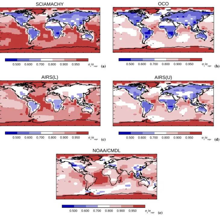
First we are interested in the uncertainty reductions gained by the different measurement concepts for PW/SC, which we consider the most realistic scenario (see Fig. 2). The blue
areas in Fig. 2 point at low fractional changes in flux uncer-tainty, indicating that the inversion obtained uncertainty re-duction is high and that the measurement system is perform-ing well. For all satellite instruments the uncertainty reduc-tions are larger over the continents than over the oceans, ow-ing to the larger prior uncertainties over land. Generally, al-most no uncertainty reduction is achieved for the Earth’s ice caps, where the prior uncertainty is set to a very low number
justified by the absence of any significant CO2 surface
ex-change there. The flask network shows a more patchy uncer-tainty reduction pattern than the satellites, explained by the uneven sampling by the heterogeneous monitoring network. The most notable uncertainty reductions occur in grid boxes where continental measurement sites are located. Over the oceans SCIAMACHY shows by far the poorest performance of all measurement systems, resulting from the assumption that no column measurements can be retrieved from this in-strument there. Measurements in sun-glint can successfully compensate for this as indicated by the results for OCO. The performance of AIRS is highly sensitive to the choice of weighting function, ranging from a performance similar to OCO for AIRS(U) to the much poorer performance for AIRS(L). Some differences between the instruments only show up for monthly uncertainty reductions (not shown). As expected, the uncertainty reductions for the sun light depen-dent instruments follow the latitudinally and seasonally vary-ing in-flux of solar radiation. The thermal IR instruments show a similar seasonality in performance, which can be ex-plained by the seasonality of its response functions (as shown in Fig.3).
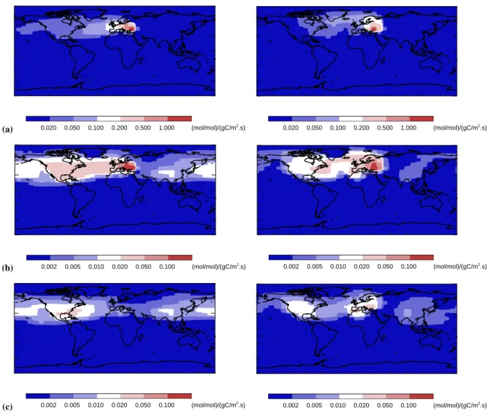
Before we analyze the contributions of the right hand side terms in Eq. (2) to the fractional changes in flux uncertainty in Fig. 2, we first focus on some relevant differences be-tween the transport matrices (A in Eq. 2). Figure 3 demon-strates how differences in measurement technique lead to differences in the measurement’s sensitivity towards surface fluxes. AIRS(L), OCO, and NOAA/CMDL were selected because they span the range from low to high sensitivity to the surface layer. Plotted are the contributions of monthly
CO2surface flux pulses released anywhere in the model
do-main to a monthly averaged measurement taken in Eastern
Europe (NOAA/CMDL site “HUN” at 47◦N and 17◦E) in
the same month as the flux pulses were released. Naturally, this response is highest near the measurement location, and decreases with the time it takes to transport (and disperse) the pulses towards this location. The more localized and intense the response, the higher the measurement’s ability to resolve the local flux and, thereby, reduce its uncertainty. Ideally a satellite measurement should only be sensitive to its footprint, then after sampling the whole globe we’d be able to perfectly resolve the fluxes on the scale of the footprint. Atmospheric mixing, however, prevents this from happen-ing. The response maximum for a surface measurement is roughly a factor of 10 higher than for a full column mea-surement (OCO) at the same location and is clearly more
SCIAMACHY 0.500 0.600 0.700 0.800 0.900 0.950 σ x/σxapr (a) OCO 0.500 0.600 0.700 0.800 0.900 0.950 σ x/σxapr (b) AIRS(L) 0.500 0.600 0.700 0.800 0.900 0.950 σ x/σxapr (c) AIRS(U) 0.500 0.600 0.700 0.800 0.900 0.950 σx/σxapr (d) NOAA/CMDL 0.500 0.600 0.700 0.800 0.900 0.950 σ x/σxapr (e)
Fig. 2. Fractional change in flux uncertainty (σx/σxpri) per year and per model grid cell gained by inversions on the basis of measurements by (a) SCIAMACHY; (b) OCO; (c) AIRS(L); (d) AIRS(U) (e) NOAA/CMDL , for process weighted and space correlated (PW/SC) prior uncertainties (see text).
localized. It implies that by measuring the total column in-stead of at the surface only we are less well able to resolve surface fluxes. For a full column measurement (OCO) this sensitivity is again about 10 times higher than for a measure-ment of only the upper half of the column (AIRS(L)). Note that, the maximum sensitivity for the latter does not occur in the same place as the measurement was taken, because that pulse is still confined to the unobserved part of the column.
As expected, the source response functions vary with at-mospheric transport conditions, as illustrated in Fig. 3 by its seasonal dependence. In first instance the atmospheric mixing of the emissions is confined to a boundary layer that is shallower in winter than in summer. In our model, this results in a response function with a ∼10% higher maxi-mum for a surface measurement in winter than in summer. The full column responses, however, are lower by ∼10% (OCO) in winter. Because the vertical weighting function
2 (a) 0.020 0.050 0.100 0.200 0.500 1.000 (mol/mol)/(gC/m2 .s) 0.020 0.050 0.100 0.200 0.500 1.000 (mol/mol)/(gC/m2 .s) (b) 0.002 0.005 0.010 0.020 0.050 0.100 (mol/mol)/(gC/m2 .s) 0.002 0.005 0.010 0.020 0.050 0.100 (mol/mol)/(gC/m2.s) (c) 0.002 0.005 0.010 0.020 0.050 0.100 (mol/mol)/(gC/m2 .s) 0.002 0.005 0.010 0.020 0.050 0.100 (mol/mol)/(gC/m2 .s)
Fig. 3. The sensitivity of the concentration at NOAA/CMDL site “HUN” (47◦N, 17◦E) as measured by (a) NOAA/CMDL; (b) OCO; (c) AIRS(L) to monthly CO2flux pulses anywhere. The measurements refer to January (left panels), and July means (right panels). The fluxes
are per grid box and are active during the same month. Note that the contour levels in panels (a) are are factor 10 higher than in panels (b) and (c).
of OCO is constant (see Fig. 1) vertical mixing only should not influence its measurements. Vertical mixing enhances the response of AIRS(L), because it transports the pulses to-wards observable altitudes. The reduced OCO response dur-ing winter can be explained by increased advection caused by a stronger jet-stream in winter than in summer. The re-sponse maxima of AIRS(L) in summer are clearly associated with convective activity over the United States and Europe
lifting the CO2pulses up to observed altitudes. As expected,
these areas of increased response have disappeared in winter, when continental convection has subsided.
instruments the regions of low and high uncertainty reduc-tion are primarily determined by the prior uncertainties, and to a lesser extent by the measurement sensitivities. This is
explained by the rather even measurement coverage by the satellites, as opposed to the NOAA/CMDL network where the uncertainty reduction patterns show a pronounced influ-ence of the network configuration. Although, the measure-ment coverage is in fact not quite even for SCIAMACHY, this doesn’t alter the patterns of uncertainty reduction much. This is because the contributions of the measurements and prior fluxes have similar large-scale patterns (distinguishing land and ocean), reinforcing each other. In other words, SCIAMACHY specifically samples those regions where we expect to be able to learn the most from additional data.
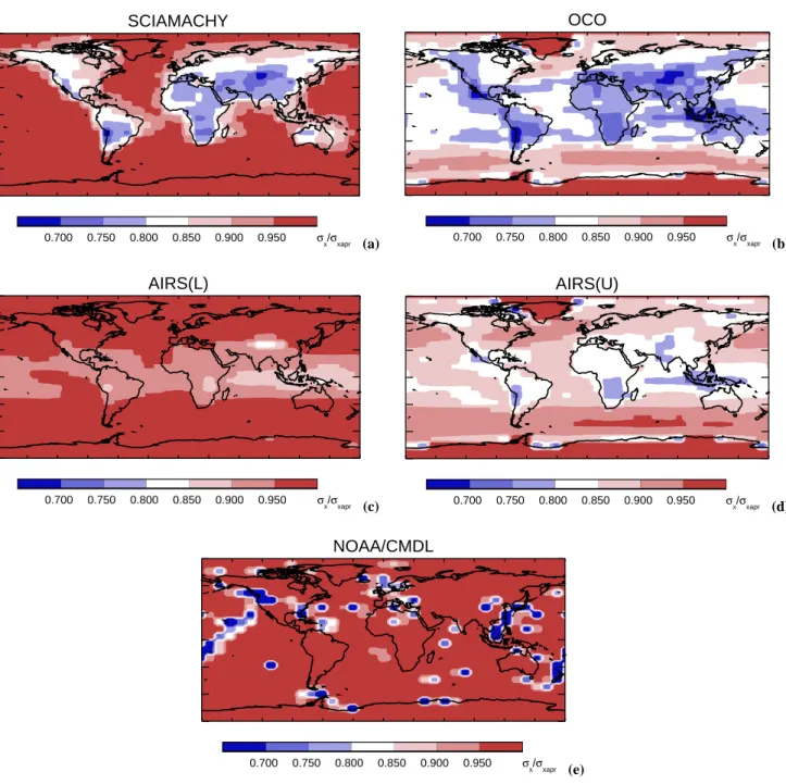
Next we will focus in more detail on the differences be-tween the different satellite instruments. To highlight these differences we use the prior uncertainty scenario EW/UC,
SCIAMACHY 0.700 0.750 0.800 0.850 0.900 0.950 σ x/σxapr (a) OCO 0.700 0.750 0.800 0.850 0.900 0.950 σx/σxapr (b) AIRS(L) 0.700 0.750 0.800 0.850 0.900 0.950 σx/σxapr (c) AIRS(U) 0.700 0.750 0.800 0.850 0.900 0.950 σ x/σxapr (d) NOAA/CMDL 0.700 0.750 0.800 0.850 0.900 0.950 σx/σxapr (e)
Fig. 4. As Fig. 2, but for evenly weighted uncorrelated (EW/UC) prior uncertainties.
which effectively eliminates the influence of the prior un-certainties on the uncertainty reduction patterns. Intuitively, it may seem more appropriate to use area weighted rather than evenly weighted uncertainties for this purpose. Weight-ing the uncertainties by area is tantamount to expressWeight-ing the problem in flux units. Since the concentration data is in units of ppm this weighting has the effect of making the concentra-tions more sensitive to a unit change in fluxes at low latitudes than high (since low latitude grid cells are larger). Because the uncertainty reduction depends on this sensitivity, low
lat-itude fluxes will incur a greater reduction in uncertainty for this rather trivial reason. We wish to isolate the impacts of atmospheric sampling and transport so use equally weighted uncertainties to eliminate this artifact. Figure 4 presents the uncertainty reductions for EW/UC scenario. Note that again the ice caps were kept at a low prior uncertainty, explain-ing why no uncertainty reduction is gained there. A notable difference with Fig. 2 is the strongly reduced land/sea con-trast for AIRS and OCO. For SCIAMACHY this feature still remains, now only reflecting the lack of measurements over
2
SCIAMACHY
8x10 degree 16x30 degree Sub-continent 1/4 Hemisphere 1/2 Hemisphere Hemisphere Globe 0.0 0.2 0.4 0.6 0.8 1.0 F ( σx / σxapr ) OCO
8x10 degree 16x30 degree Sub-continent 1/4 Hemisphere 1/2 Hemisphere Hemisphere Globe 0.0 0.2 0.4 0.6 0.8 1.0 F ( σx / σxapr ) (a) (b) AIRS(L)
8x10 degree 16x30 degree Sub-continent 1/4 Hemisphere 1/2 Hemisphere Hemisphere Globe 0.0 0.2 0.4 0.6 0.8 1.0 F ( σx / σxapr ) AIRS(U)
8x10 degree 16x30 degree Sub-continent 1/4 Hemisphere 1/2 Hemisphere Hemisphere Globe 0.0 0.2 0.4 0.6 0.8 1.0 F ( σx / σxapr ) (c) (d)
Fig. 5. Globally and annually averaged fractional change in flux uncertainty (σx/σxpri) as a function of temporal and spatial scale, for (a) SCIAMACHY; (b) OCO; (c) AIRS(L); (d) AIRS(U), Green, annually integrated fluxes; red, seasonally integrated fluxes; black, monthly fluxes. Dashed and solid lines refer satellite instruments and to the NOAA/CMDL network, respectively. Prior uncertainties are process weighted and space correlated (PW/SC).
the oceans. Note that for this instrument the uncertainty re-ductions over the oceans are smaller compared with PW/SC, despite the fact that the oceanic prior uncertainties are larger (the globally integrated prior flux uncertainties for PW/SC and EW/UC are the same). This is explained by the fact that the prior uncertainties are now uncorrelated, while they were spatially correlated before. When using spatial corre-lations the uncertainty reductions are partially “shared” with neighboring fluxes, which does not happen here anymore. This effect is even more pronounced for the surface network, from which we can now clearly identify the measurement lo-cations. Generally, areas of increased uncertainty reduction seem to be associated with increased surface elevation (e.g. Andes and Himalaya) and convection (Indonesia). Particu-larly in case of AIRS(L) a relationship with surface elevation makes sense, because for high enough mountains the instru-ment would actually see the surface. The storm tracks of the northern and southern hemisphere show up, coinciding with decreased uncertainty reductions. This can most likely be attributed to reduced responses resulting from enhanced
mixing by traversing low pressure systems. We can exclude the influence of clouds, because AIRS was assumed to have a weekly measurement everywhere regardless of cloud cover. It may be surprising that also for SCIAMACHY and OCO the effects of cloud cover seem absent. This is explained by the number of measurements per weekly ensemble that is generally large enough to reduce the uncertainties to values near the assumed 1 ppm minimum (see Sect. 2.2). A conse-quence of this approach is that it almost eliminates the influ-ence of variable cloud cover, which will not happen in real-ity. Of course, assuming the systematic error to be constant is not realistic either. This indicates the level of detail that, although relevant, we cannot properly address at present.
3.2 Scale dependence
It should be realized that the results of the previous section apply to the particular temporal and spatial scales that were selected. Here we analyze how the uncertainty reductions vary as a function of scale. For this purpose we integrated the prior and posterior uncertainties over various scales and then
AIRS(L)
8x10 degree 16x30 degree Sub-continent 1/4 Hemisphere 1/2 Hemisphere Hemisphere Globe 0.0
0.5 1.0 1.5 2.0
Relative flux uncertainty reduction (-)
OCO
8x10 degree 16x30 degree Sub-continent 1/4 Hemisphere 1/2 Hemisphere Hemisphere Globe 0.0
0.5 1.0 1.5 2.0
Relative flux uncertainty reduction (-)
(a) (b)
SCIAMACHY
8x10 degree 16x30 degree Sub-continent 1/4 Hemisphere 1/2 Hemisphere Hemisphere Globe 0.0
0.5 1.0 1.5 2.0
Relative flux uncertainty reduction (-)
NOAA/CMDL
8x10 degree 16x30 degree Sub-continent 1/4 Hemisphere 1/2 Hemisphere Hemisphere Globe 0.0
0.5 1.0 1.5 2.0
Relative flux uncertainty reduction (-)
(c) (d)
Fig. 6. As Fig. 5, expressed as uncertainty reductions relative to AIRS(U) ([1 − σx/σxpri]X/[1 − σx/σxpri]AI RS(U )). X refers to: Panel (a),
AIRS(L); panel (b), OCO; panel (c), SCIA; panel (d), NOAA/CMDL. The solid lines show satellite results for the PW/SC scenario, dashed lines for PW/UC.
averaged the obtained uncertainty reductions over the globe and over 1 year. The selected temporal and spatial scales are:
(i) monthly, seasonal, annual, and (ii) 8◦×10◦(grid scale),
16◦×30◦ (2×3 grid cells), sub-continental, quarter
Hemi-sphere, half HemiHemi-sphere, HemiHemi-sphere, and the Globe. The sub-continental scale refers to the 11 land and 11 ocean re-gions that were used in TRANSCOM 3 (Gurney et al., 2002). Contributions of the ice caps were excluded from the global averages derived at any scale. Like in the previous subsec-tion we choose to weigh each integrated region by its number of grid cells, which was done mainly for consistency. It turns out that the choice for area or grid weighing does alter the results somewhat. In addition, the specific choice of scale and the shapes of the integrated regions affect some details of the outcome. Care is taken, however, to only interpret those aspects of the results that proved robust to such arbi-trary choices.
Figure 5 shows the scale dependence of the globally and annually averaged uncertainty reduction for each instrument using PW/SC prior uncertainties. Generally, uncertainty re-ductions increase with scale, owing to the fact that the larger
scales are observed by larger numbers of measurements and at those scales regions can better be distinguished from their neighbors (i.e. are easier to resolve). Interestingly, this ap-plies to a lesser extent to changes in temporal than in spatial scale, suggesting that the smallest considered time scale is better resolved than the smallest spatial scale. This is true in particular for the weekly satellite measurements, except for SCIAMACHY which is due probably to contributions of oceanic regions that are poorly resolved by this instrument. For the assumed measurement uncertainties the satellites out-perform the reference network on most scales. This result may not prove robust though, since, like we mentioned ear-lier, the measurement uncertainties for the satellites are still debated and are most likely too optimistic. The scale depen-dence, however, is expected to be more reliable, unless it is significantly affected by the neglect of satellite measurement correlations. We did not feel confident speculating on these correlations, and acknowledge that this factor may limit the applicability of these results.
As can be seen in Fig. 5 the decrease of the fractional change in flux uncertainty with scale has a rather similar
2 GLOBE 0 5 10 15 20 measurement precision (ppmv) 0.0 0.2 0.4 0.6 0.8 1.0 F ( σx / σxapr ) LAND 0 5 10 15 20 measurement precision (ppmv) 0.0 0.2 0.4 0.6 0.8 1.0 F ( σx / σxapr ) TROPICAL LAND 0 5 10 15 20 measurement precision (ppmv) 0.0 0.2 0.4 0.6 0.8 1.0 F ( σx / σxapr )
Fig. 7. Fractional change in flux uncertainty on the basis of SCIA-MACHY measurements for different spatial scales as a function of measurement precision (PW/SC scenario). The uncertainties have been averaged globally and annually (top panel), over land only (middle panel), and over tropical land only (bottom panel). The scales range from 8◦×10◦ (black), 16◦×30◦ (red), to sub-continental (green). Horizontal lines indicate the corresponding un-certainties for NOAA/CMDL.
shape for all measurement systems. By plotting the ratios of uncertainty reductions for two instruments the differences become more pronounced (see Fig. 6). Values higher (lower) than 1 indicate that a given instrument is performing bet-ter (worse) than AIRS(U). We have chosen to divide by the AIRS(U) because this instrument shows a rather straight for-ward relation between posterior uncertainty and scale, un-like for example the surface network where the inhomoge-neous sampling adds complexity to this relationship. On the global scale the performances of all satellite instruments are quite comparable, but, interestingly, they divert towards smaller scales. This is most obvious for AIRS(L) and OCO, that show respectively decreased and increased uncertainty reductions going towards smaller scales as compared with AIRS(U). Since the vertical weighting function is the main difference between these instruments, it indicates that the in-struments ability to resolve smaller scales is related to its sen-sitivity to low altitudes.
Although the NOAA/CMDL network is more sensitive near the surface than any of the satellite instruments, its scale dependence is in fact not much different from AIRS(U). This is because the satellite instruments sample almost any location on the globe, while the surface network is at large distance of many fluxes which also reduces the cor-responding sensitivities. In a comparison of AIRS(U) and NOAA/CMDL these counteracting factors largely cancel out, which is also true for SCIAMACHY and NOAA/CMDL. We tested how a smaller surface network influences this bal-ance (not shown). Then, as expected, the performbal-ances of SCIAMACHY and AIRS improve towards smaller scales rel-ative to the reduced surface network.
Interestingly, the relation between uncertainty reduction and scale is also influenced by the assumed correlation of the prior uncertainties as can be seen by comparing the solid and dashed lines in Fig. 6. Generally, positively correlated prior flux uncertainties reduce the scale dependence of the uncertainty reductions.
3.3 Precision requirements
Finally, we quantify the threshold uncertainty that would be needed for the SCIAMACHY instrument to outperform the current surface network, in a similar fashion as first presented by Rayner and O’Brien (2001) (see Fig. 7). In addition, the scale dependences that were presented earlier allow us to generalize this plot by showing this threshold uncertainty as a function of spatial scale. The variation of the thresh-old with scale turns out to be rather small, as expected from the results that were presented in the previous subsection. For the SCIAMACHY instrument the break even point for globally and annually averaged sub-continental scale fluxes is at 3–4 ppm. For the OCO instrument this threshold mix-ing ratio is roughly a factor 2 higher (not shown). Note that these uncertainties refer to single column measurements. In our highly simplified statistical model the uncertainties of the
weekly 8◦×10◦ measurement ensembles are roughly a
fac-tor 3.5 lower. An important point to note, particularly for SCIAMACHY, is the dependence of the threshold measure-ment precisions on the part of the globe over which the flux uncertainty reductions were averaged. For example, by se-lecting only the continents the SCIAMACHY thresholds in-crease by about a factor of 5. A further inin-crease of 15 to 18 ppm is obtained after selection of the tropical continents
(between 30◦N and 30◦S). For some regions the thresholds
reach even higher values, for example of 20–25 ppm over the Amazon and tropical Africa.
4 Discussion
This study confirms the conclusions by Rayner and O’Brien (2001) and Pak and Prather (2001) that rather precise satel-lite measurements are needed to obtain constraints on global
CO2sources and sinks that are similar to those currently
ob-tained from surface sampling networks. For the instruments that were tested in this study it is estimated that the required
precisions are in the range of 1–2 ppm for weekly 8◦×10◦
measurement ensembles and sub-continental scale fluxes. In the recent literature, measurement precisions between 0.3 and 6 ppm are reported for single column near IR measure-ments (Dufour and Breon, 2003; Kuang et al., 2002; Aoki et al., 2002), and 1 to 3.6 ppm for ensemble averaged thermal IR measurements (Ch´edin et al., 1998; Engelen et al., 2001) indicating that such requirements might be feasible. Obvi-ously it remains to be seen how close the performance of the real instruments can get to these theoretical values. However, our analyses also indicate that regionally the required preci-sion to match the present surface network may relax by as much as a factor of 6. Those regions are mainly located over land, because the continents are relatively poorly sampled by surface networks. This is of particular interest to carbon cy-cle research, because the land is generally where additional measurements are most urgently needed. As pointed out by Pak and Prather (2001), satellite measurements are expected to be particularly useful over tropical continents where the
CO2sources and sinks are most uncertain. Because the
per-formances of satellite instruments and the surface network maximize in different regions, added value is expected from
their combined use in a single atmospheric inversion of CO2
sources and sinks. This might work particularly well for the combination of SCIAMACHY and NOAA/CMDL network. While the first measures predominantly over the continents, with only limited measurement capability over the oceans, the opposite is true for the second. Combining different sources of measurements in an inversion, however, is not a trivial exercise because of possible differences in calibration. Spatial and temporal resolution has been examined as an-other measure of satellite performance. As mentioned earlier, resolution is related to the scale dependence of the
inversion-derived uncertainty reductions. Negative correlations
be-tween unresolved regions cause their sum to be relatively well constrained in comparison with the individual regions. This explains the uncertainty decrease with increasing scale that is seen, for example, in Fig. 5. The steeper the slope, the stronger the anti-correlations. If the posterior uncertain-ties were correlated just like the prior uncertainuncertain-ties, a hori-zontal line would be obtained at some level determined by the measurement precision. Atmospheric mixing causes the posterior fluxes to become more anti-correlated. Generally, the uncertainty reductions for the satellites decrease fairly rapidly at smaller scales, indicating that their ability to re-solve small scale features is limited. Since this behavior is sensitive to the shape of the vertical weighting function, it can be concluded that by measuring the full column instead of at the surface the achievable spatial resolution is reduced. Note that our inversion set-up is not suitable for estimating the maximum achievable resolution, because we aggregated the measurements to the grid of a rather coarse resolution model. Similar limitations are introduced by the specified time discretizations. Hence we do not exploit the full in-formation content of the measurements, in particular, on the smallest scales. It may well be, however, that by measur-ing total column averaged mixmeasur-ing ratios the achievable hori-zontal resolution is already lower than the size of the obser-vational footprints. This could of course be verified using a highly resolved meso-scale atmospheric transport model. First, however, we should find out which are the relevant scales that need to be resolved to answer carbon cycle re-lated questions. For the terrestrial biosphere these requiments seem rather stringent, since we’d ideally want to re-solve the scale of ecosystems which can be much smaller
than our 8◦×10◦. However, given our coarse
understand-ing in many sparsely monitored parts of the world, there is still much left to be learned on much larger scales. At this stage, full continental coverage is probably of more impor-tance than the ability to resolve relatively small scales. This argument still favors a small footprint, because this increases the fraction of cloud free observations, and thereby spatial coverage.
Unfortunately our results do not allow a clear statement about the relative performance of near IR and thermal IR techniques. This is because of the substantial range in per-formance spanned by AIRS(L) and AIRS(U), indicating that its performance is in fact rather uncertain. It does, how-ever, show that performance of the thermal IR technique is
quite sensitive to the instruments ability to measure CO2
at altitudes below 500 hPa. If this sensitivity is only mod-estly reduced (as in AIRS(U)) the loss in performance can be compensated by a relatively large number of measure-ments. It is questionable, however, to what extent thermal IR instruments will really be able to reach the surface sen-sitivities of AIRS(U). For example, the shortest wavelengths (∼4 µm) that contribute most to the surface signal cannot be measured during daytime, because interference by reflected sunlight becomes significant (ACECHEM, 2001). On the
2
other hand, during nighttime the continental boundary layer is much shallower, so that the measurements should reach even lower altitudes. Again there may be additional value in combining several measurement concepts. By measuring in the near and thermal infrared we might not only be able to see the planetary boundary layer, but also measure its con-centration difference with the free troposphere, which sounds highly attractive.
Our results clearly indicate that SCIAMACHY’s perfor-mance is reduced by its inability to measure over the oceans. Although the instrument hasn’t been designed to keep track of the sun-glint region like OCO, it does receive sporadic
measurements in sun-glint. These measurements are all
within a narrow latitude band near the tropics that varies sea-sonally. Their contribution to the instrument’s overall per-formance will, however, not be significant, which is why they have been neglected here. Not surprisingly, the lack of ocean measurements leads to a poor performance of the
at-mospheric inversion over the oceans. On the 8◦×10◦scale,
the estimates over land are not much influenced by this, pointing at a rather local nature of the constraints that induce the significant uncertainty reductions at this scale. Integrated over the globe, however, the benefits of ocean measurements are evident for all the analyzed scales.
A shortcoming of the presented instrument comparison is the rather crude description of measurement uncertainty. Ex-cept for the instrument’s radiometric noise this is determined
by the uncertainties in the retrieval of CO2 from the
mea-surements. The latter is influenced by knowledge on vari-ous physical and chemical properties of the measured atmo-spheric column. Here we have assumed that the errors will be comparable for near IR and thermal IR techniques. This may not be the case since these instruments are sensitive to atmospheric parameters that are quite different. Thermal IR measurements are sensitive to uncertain vertical profiles of temperature and humidity. For near infrared measurements, however, interference by aerosols and thin cirrus clouds are expected to be more critical. The achievable measurement precision will be determined by our ability to characterize and correct these factors. For example, it has been sug-gested that the effective air-mass that is sampled by a single column measurement (air-mass factor) can be quantified by measuring oxygen (O’Brien and Rayner, 2002) or, in sun-glint observations, by measuring polarized radiances (Aoki et al., 2002). The effectiveness of these procedures, how-ever, has still to be demonstrated using real data. Another and potentially important limitation is the assumption of un-correlated measurement uncertainties. Many instrument re-lated uncertainties (optics, detectors, electronic circuits) and path related uncertainties (cirrus clouds, aerosols, tempera-ture profiles), however, will likely have systematic compo-nents. This reduces the gain in precision that is obtained by co-adding or averaging large numbers of measurements. In addition, it changes the scale dependent uncertainty reduc-tions presented in the previous section such that it reduces
the increasing uncertainty reduction with increasing scale. Last but not least it should be mentioned that the atmo-spheric transport model is assumed to be perfect, while obvi-ously it isn’t. In particular vertical mixing is known to vary across the models, reflecting the relatively large uncertainties that are associated with the parameterizations of convection and turbulent mixing (Denning et al., 1999). This may have important implications for satellite instruments that are sensi-tive to the shape of the vertical concentration profile (such as AIRS). In absence of a height dependent sensitivity, the col-umn averaged concentrations may rather be less susceptible to transport model uncertainties than surface concentrations, as pointed out by Rayner and O’Brien (2001). Related to ver-tical mixing is a tendency of many transport models that use diagnosed winds (e.g. from ECMWF or NCEP) to simulate mean “ages” of stratospheric air that are much younger than the measurements indicate (Andrews et al., 2001; Jones et al., 2001). This may lead to large scale off-sets in the inversion-derived flux estimates.
5 Conclusions
We studied the potential benefit of satellite instruments that
measure atmospheric CO2 mixing ratios for the estimation
of CO2 sources and sinks by inverse modeling. Three
hy-pothetical instrument types have been compared, inspired by currently operational and planned missions. The rela-tive performance of these instruments is quantified by syn-thetic simulations of their ability to reduce the uncertainty
in the current CO2 source and sink estimates. These
per-formances are put in perspective by comparison to the cur-rent NOAA/CMDL flask sampling network. The thermal IR instrument AIRS has the advantage of relatively high number of measurements, leading to a notably better per-formance over the oceans than SCIAMACHY. This short-coming of SCIAMACHY can be compensated by measur-ing in sun-glint, as demonstrated by OCO. An uncertain fac-tor of AIRS, however, is its ability to measure at low alti-tudes which is demonstrated to be of crucial importance. For the near IR instruments SCIAMACHY and OCO the surface sensitivity will certainly be more favorable. Overall OCO is the most promising satellite concept of those tested be-cause it is a near IR instrument, which measures in sun-glint over the oceans. This result was obtained despite a relatively conservative precision assumption for the OCO instrument. The performance of the instruments is shown to vary geo-graphically, as determined by the assumed prior uncertain-ties, measurement uncertainuncertain-ties, and atmospheric transport properties. Enhanced horizontal mixing reduces the perfor-mance by effectively dispersing the concentration gradients. Convection, on the contrary, is advantageous to instruments that are insensitive to the lower altitudes. Generally, the geo-graphical differences suggest that additional benefits can be obtained from the combined use of satellite instruments and
surface networks, provided that systematic differences can be accounted for. We have shown that the instrument perfor-mances should be quantified with reference to the considered scale, as they vary as a function of temporal and spatial scale. Generally the performance improves going to larger scales, as these scales become progressively better constrained by the increasing number of measurements addressing them. In-creased sensitivity near the surface increases the instruments ability to resolve smaller scales. The scale dependence of the satellite instruments is rather comparable to that of the sur-face network, with a slight improvement for satellites that are sensitive to the surface and reach full global coverage (OCO and AIRS(U)). In line with earlier studies, the required
pre-cision of weekly columns of CO2on 8◦×10◦needed to
im-prove the inversion-derived annual flux estimates on a sub-continental scale over the whole globe is less than 1% (or 3.5 ppm) for all instruments. For OCO this requirement is a factor 2 less stringent than for SCIAMACHY (2 versus 1 ppm). The SCIAMACHY requirements, however, relax by a factor of 5 if only the continents are taken into account. We anticipate that SCIAMACHY can contribute most
sig-nificantly to our estimates of CO2fluxes over tropical
conti-nents. This study relies heavily on the assumed precision of satellite measurements, which is poorly quantified at present. This is not only a limitation of our synthetic approach, but, unless the error assessments improve significantly, this sit-uation will remain when real data are available. Therefore, we’d like to emphasize that a reliable uncertainty assessment is vital to any interpretation of these measurements using in-verse modeling. In particular the identification of random and systematic components should receive high priority.
Acknowledgements. We acknowledge fruitful discussions within
the COCO project, and are particularly grateful to R. Engelen (ECMWF) and C. Crevoisier (LMD). Further, we’d like to thank A. Maurellis and H. Schrijver (SRON) for useful support. P. Rayner and K. Gurney provided constructive and valuable reviews of this paper. This study was financially supported by the EC project COCO (EVG1-CT-2001-00056) and LSCE, with special thanks to Philippe Ciais for initiating this work.
Edited by: P. Kasibhatla
References
ACECHEM: Atmospheric composition explorer for chemistry and climate interactions, SP-1257 4, ESA, 2001.
Andres, R. J., Marland, G., Fung, I., and Matthews, E.: A 1◦×1◦ distribution of carbon dioxide emissions from fossil fuel con-sumption and cement manufacture, 1950–1990, Global Biogeo-chemical Cycles, 10, 419–429, 1996.
Andrews, A. E., Boering, K. A., Wofsy, S. C., Daube, B. C., Jones, D. B., Alex, S., Loewenstein, M., Podolski, J. R., and Strahan, S. E.: Empirical age spectra for the midlatitude lower strato-sphere from in situ observations of CO2: Quantitative evidence
for a subtropical “barrier” to horizontal transport, J. Geophys. Res., 106, 10 257–10 274, 2001.
Aoki, T., Aoki, T., and Fukabori, M.: Path-radiance correction by polarization observation of Sun glint glitter for remote mea-surements of tropospheric greenhouse gases, Applied Optics, 24, 2002.
Aumann, H. H. and Pagano, R. J.: Atmospheric infrared sounder on Earth observing system, Optical Eng., 33, 776–784, 1994. Bousquet, P., Peylin, P., Ciais, P., Quere, C. L., Friedlingstein, P.,
and Tans, P. P.: Regional changes in carbon dioxide fluxes of land and oceans since 1980, Science, 290, 1342–1346, 2000. Bovensmann, H., Burrows, J. P., Buchwitz, M., Frerick, J., No¨el,
S., Rozanov, V. V., Chance, K. V., and Goede, A. P. H.: SCIA-MACHY: Mission objectives and measurement modes, J. Atmos. Sci., 56, 127–150, 1999.
Ch´edin, A., Saunders, R., Hollingsworth, A., Scott, N., Matricardi, M., Etcheto, J., Clerbaux, C., Armante, R., and Crevoisier, C.: The feasibility of monitoring CO2from high resolution infrared
sounders, J. Geophys. Res., 108, doi:10.1029/2001JD001 443, 1998.
Ch´edin, A., Hollingsworth, A., Scott, N. A., Serrar, S., Crevoisier, C., and Armante, R.: Annual and seasonal variations of at-mospheric CO2,N2O and CO concentrations retrieved from
NOAA-TOVS satellite observations, Geophys. Res. Lett., 29, doi:10.1029/2001GL14 082, 2002.
Ch´edin, A., Serrar, S., Scott, N. A., Crevoisier, C., and Armante, R.: First global measurement of midtropospheric CO2 from
NOAA polar satellites: Tropical zone, J. Geophys. Res., 108, doi:10.1029/2003JD003 439, 2003.
Conway, T. J., Tans, P. P., Waterman, L. S., and Thoning, K. W.: Evidence for interannual variability of the carbon cycle from the national oceanic and atmospheric administration climate moni-toring and diagnostics laboratory global air sampling network, J. Geophys. Res., 99, 22 831–22 855, 1994.
Denning, A. S., Holzer, M., Gurney, K. R., et al.: Three-dimensional transport and concentration of SF6: A model
in-tercomparison study (Transcom 2), Tellus, Ser. B, 51, 266–297, 1999.
Dufour, E. and Breon, F.-M.: Spaceborne estimate of atmospheric CO2 column using the differential absorption method: Error
analysis, Appl. Optics, 42, 3595–3609, 2003.
Engelen, R. J., Scott Denning, A., Gurney, K. R., and Stephans, G. L.: Global observations of the carbon budget, 1. Expected satellite capabilities in the EOS and NPOESS eras, J. Geophys. Res., 106, 20 055–20 068, 2001.
Enting, I. G., Trudinger, C. M., and Francey, R. J.: A synthesis in-version of the concentration and δ13C of atmospheric CO2,
Tel-lus, Ser. B, 47, 35–52, 1995.
Gurney, K. R., Law, R. M., Denning, A. S., et al.: Towards robust regional estimates of CO2sources and sinks using atmospheric
transport models, Nature, 415, 626–630, 2002.
Heimann, M. and K¨orner, S.: The global atmospheric tracer model TM3, Model description and user’s manual release 3.8a, Max Planck Institute of Biogeochemistry, 2003.
House, J. I., Prentice, I. C., Ramankutty, N., Houghton, R. A., and Heimann, H.: Reconciling apparent inconsistencies in estimates of terrestrial CO2sources and sinks, Tellus, Ser. B, 55, 345–363,


![Fig. 6. As Fig. 5, expressed as uncertainty reductions relative to AIRS(U) ( [ 1 − σ x /σ xpri ] X / [ 1 − σ x /σ xpri ] AI RS(U ) )](https://thumb-eu.123doks.com/thumbv2/123doknet/13044788.382676/12.892.88.801.91.583/fig-fig-expressed-uncertainty-reductions-relative-airs-xpri.webp)

