Conformational Dynamics in Ion Mobility Data

HAL Id: hal-01501246

https://hal.archives-ouvertes.fr/hal-01501246

HAL is a multi-disciplinary open access archive for the deposit and dissemination of sci-entific research documents, whether they are pub-lished or not. The documents may come from teaching and research institutions in France or abroad, or from public or private research centers.

L’archive ouverte pluridisciplinaire HAL, est destinée au dépôt et à la diffusion de documents scientifiques de niveau recherche, publiés ou non, émanant des établissements d’enseignement et de recherche français ou étrangers, des laboratoires publics ou privés.

Conformational Dynamics in Ion Mobility Data

Salomé Poyer, Clothilde Comby-Zerbino, Chang Min Choi, Luke Macaleese,

Claire Deo, Nicolas Bogliotti, Juan Xie, Jean-Yves Salpin, Philippe Dugourd,

Fabien Chirot

To cite this version:

Salomé Poyer, Clothilde Comby-Zerbino, Chang Min Choi, Luke Macaleese, Claire Deo, et al.. Con-formational Dynamics in Ion Mobility Data. Analytical Chemistry, American Chemical Society, 2017, 89 (7), pp.4230-4237. �10.1021/acs.analchem.7b00281�. �hal-01501246�

1

Analytical Chemistry 2017, DOI: 10.1021/acs.analchem.7b00281

Conformational Dynamics in Ion Mobility Data

Salomé Poyer,1† Clothilde Comby-Zerbino,2 Chang Min Choi,2‡ Luke MacAleese,2 Claire Deo,3 Nicolas Bogliotti,3 Juan Xie,3 Jean-Yves Salpin,1 Philippe Dugourd,2 and Fabien Chirot4*

1. LAMBE, Université Evry Val d’Essonne, CEA, CNRS, Université Paris-Saclay, F-91025, Evry, France 2. Univ Lyon, Université Claude Bernard Lyon 1, CNRS, Institut Lumière Matière UMR 5306, F-69100, Villeurbanne, France

3. PPSM, ENS Paris-Saclay, CNRS, Université Paris-Saclay, F-94235 Cachan, France

4. Univ Lyon, Université Claude Bernard Lyon 1, Ens de Lyon, CNRS, Institut des Sciences Analytiques UMR 5280, 5 rue de la Doua, F-69100, Villeurbanne, France

Supporting Information Available: Details of the derivation of equations (15) and (16). Experimental and simulated ATDs at 287 K, 297 K, and 312 K for different trapping delays.

Corresponding Author

Present Addresses

† Aix Marseille Univ, CNRS, ICR, Marseille, France.

‡ Mass Spectrometry & Advanced Instrumentation Group, Korea Basic Science Institute (KBSI), Chungbuk, Republic of Korea.

Abstract

The shape of the spectral features in arrival time distributions (ATDs) recorded by ion mobility spectrometry (IMS) can often be interpreted in terms of the co-existence of different isomeric species. Interconversion between such species is also acknowledged to influence the shape of the ATD, even if no general quantitative description of this effect is available. We present an analytical model that allows simulating ATDs resulting from interconverting species. This model is used to reproduce experimental data obtained on a bi-stable system, and to interpret discrepancies between measurements on different types of instruments. We show that the proposed model can be further exploited to extract kinetic and thermodynamic data from tandem-IMS measurements. Ion mobility spectrometry (IMS) is now widely used in combination with mass spectrometry (MS) for its ability to separate species in the gas phase as a function of their “surface-to-charge ratio”. As a separation technique coupled to MS, IMS has the advantage to allow decongestion of the mass spectra, and the timescales of the IMS analysis are compatible with online coupling to upstream chromatographic techniques, which makes it a powerful tool in the frame of high throughput methods for complex mixtures analysis.1,2 Beyond separation, the possibility to extract structural information from IMS measurements has also been widely exploited to study the intrinsic conformational properties of isolated molecular compounds, especially peptides, proteins, and

2

biomolecular complexes.3–6 Indeed, IMS/MS is now recognized as a useful tool for structural biology, in particular for the determination of the architecture of large protein complexes.7,8

The classical workflow for structure elucidation based on IMS relies on the measurement of the average momentum transfer cross section (CCS) for collisions between molecular ions and buffer gas. Using drift tube instruments, the CCS Ω is directly related to the drift time 𝑡Dof the ions in the buffer

gas:9 𝑡D = 16 3 √ 𝜇𝑘_B𝑇 2𝜋 𝑁𝐿 𝑞𝐸Ω (1)

where 𝜇 is the reduced mass for ion-buffer gas collisions, 𝑁 is the number density of the gas, 𝐿 is the drift length, 𝐸 is the drift field, 𝑞 is the charge of the ion, 𝑇 is the temperature, and 𝑘B is the

Boltzmann constant.

The comparison of the experimental CCS with values estimated for candidate structures from molecular simulations, or deduced via complementary structural techniques (e.g. crystallography) allows excluding certain types of conformations, and in favorable cases to assign a structure to the observed species. When such unambiguous assignation is not achievable, IMS nevertheless provides insight in the structural diversity of the investigated systems through the shape of the measured arrival time distributions (ATDs). Namely, the presence of several peaks in the ATD for one species is often related to the coexistence of different conformational families with distinct CCS. Moreover, spectral features broader than the expected peak width, which can be estimated based on the instrument resolution, may also be interpreted as originating from different structures.

Such interpretation of the shape of the ATD in terms of conformational diversity holds as long as the structure of the investigated systems can be considered as rigid, at least during the timescale of the IMS measurement (typically 1 to 100 ms). Examples of the signature of structural transitions during the drift have been reported in the case of clusters, nucleotides, and peptides.10–12 Of course, only transitions which induce significant modification of the CCS are visible to IMS. However, the dynamics of the structural change is also important. It is generally admitted that interconversion processes that are much faster than the timescale of the measurement are basically invisible in the ATD.13 This can be easily understood in the case of a system that can adopt two structures A and B, with 𝑡A and 𝑡B the arrival times associated to a frozen system in state A and B, respectively. If the

average interconversion rate between the two states is large compared to the inverse average drift time, all ions experience a large number of interconversion events during their flight. As a consequence, all ions fly during the same time 𝑡av, corresponding to a weighted average between 𝑡A

and 𝑡B. The resulting ATD then displays a single peak, even if two interconverting species are present.

Since the position of this peak reflects the populations in each accessible state, the value of 𝑡av is

related to the equilibrium constant for the interconversion reaction 𝐴 ⇆ 𝐵. Thermodynamic quantities for this reaction (i.e. transition enthalpy and entropy) can thus be extracted from the evolution of 𝑡av as a function of the drift temperature in the case of a bi-stable system.12

Exploitation of the impact of structural transitions on the shape of the ATD was also reported in the limit of slow interconversion. More precisely, the case has been considered where transitions can occur from one conformational state A to another state B during the drift, the reverse process being

3

negligible. Such a situation was reported for different classes of systems, in particular by the group of M. Jarrold.10,12 In this case the shape of the ATD, including the contribution from ions experiencing at most one structural transition during their drift, can be reproduced by a relatively simple model. It consists in assuming a constant transition rate 𝑘. The probability that an ion initially in state 𝐵 experiences a transition 𝐵 → 𝐴 between the time 𝜏 and 𝜏 + d𝜏 during its drift is then 𝑘d𝜏e−𝑘𝜏. The resulting total drift time along the distance 𝐿 can be determined by considering that the ion has been flying at a constant velocity v𝐵 from t=0 to t=𝜏, and at a velocity v𝐴 for the rest of its flight, i.e. over a

distance 𝐿 − v𝐵𝜏. The simulated drift time distribution 𝑆(𝑡) can finally be obtained by summing over

all possible values for 𝜏, and by convoluting the resulting average drift time distribution with the expected Gaussian shape of the peaks expected from Fick’s laws for diffusion:10

𝑆(𝑡) = 𝐴0 √2𝜋𝑤e −(𝑡−𝑡_2𝑤A₂)2₊𝐵0e−𝑘𝑡B √2𝜋𝑤 e −(𝑡−𝑡_2𝑤B₂)2 +𝑘𝐵0 2𝛾 e−𝑘(𝑡−𝜃)(erf ( 𝑡B+ 𝛽 − 𝑡 √2𝑤 ) − erf ( 𝑡A+ 𝛽 − 𝑡 √2𝑤 )) (2)

where erf is the error function, 𝐴0 and 𝐵0 are the initial populations in states A and B, respectively,

𝑤 =1₂(𝑡A+ 𝑡B)√2𝑘_𝑞𝑉B𝑇 accounts for the natural width of the ion packet due to diffusion.9 The

dimensionless constant 𝛾 = 1 − 𝑡A/𝑡B, and the time constants 𝛽 =𝑘𝑤

2

𝛾 , and 𝜃 = 𝛽

2+ 𝑡A have been

introduced for simplification. The first two terms correspond to ions undergoing no interconversion during their flight. The contribution of 𝐵 → 𝐴 interconversion is represented by the third term. The above function is analytical, and depends only on known quantities, but the reaction rate. It can thus be used to fit experimental data with the transition rate as the only free parameter, thus allowing its determination. In addition, by performing temperature-dependent experiments, an Arrhenius activation energy can be obtained from the temperature dependence of 𝑘.10

Beyond the measurement of rate constants or activation energies, a proper description of the influence of interconversion dynamics on the shape of ATDs is central to properly interpret IMS data. It is particularly important for temperature-dependent measurements,13 but also for the comparison of IMS profiles obtained using different instruments, potentially associated to different activation conditions for the ions.14,15

In the present paper we present a model that allows simulating ATDs for interconverting systems valid for any value of the interconversion rate, in particular within the intermediate timescale regime that was not covered by the above discussed descriptions. Based on this model, we study the interconversion dynamics of mobility-selected molecular systems based on tandem-ion mobility measurements.

Experimental Section

Ion mobility measurements

Tandem-IMS experiments were done using a custom dual-drift tube instrument described in details elsewhere.16 Briefly, for tandem-IMS measurements, electrosprayed ions are first trapped in a funnel ion trap before injection in a first drift tube. At the end of the tube, mobility selection is achieved

4

using an electrostatic gate that lets through only ions within a narrow drift time range. The selected ions are then trapped for a controlled amount of time in a second ion funnel, and injected in a second drift tube. Finally, a series of transfer optics are used for transmission to the extraction zone of the orthogonal time-of-flight mass spectrometer used for detection. Mass spectra are recorded as a function of the drift time in the second drift tube, which allows extracting ATDs for any considered range of m/z. All the measurements herein were done using 4.0 Torr helium as a drift gas. The drift voltages across the two identical 79 cm drift tubes were typically 450 V. The drift temperature was controlled through the circulation of silicon oil (Sil100, Thermo Fisher) in the walls of the chamber housing the tubes, using a thermalized circulator (WiseCircu P30, Witeg). The temperature of the walls was measured at 4 different points along the chamber. For IMS measurements, we ensured that the maximum difference between the measured temperature at different points was below 1 K. Additional IMS measurements were performed on a travelling-wave instrument (Synapt G2-Si HDMS, Waters). For the data shown herein, the following settings were used: capillary voltage 2.5 kV, sampling cone 30 V, source temperature 50°C, desolvation gas temperature 100°C and N2

desolvation flow rate 450 L.hr−1. IMS conditions were as follows: wave velocity 800 m.s−1, wave height 40 V, N2 IMS gas flow 90 mL.min−1 (3.09 mbar), and Helium cell gas flow 180 mL.min−1.

Experiments were carried out in positive ionization mode in the ‘V’ resolution mode using the m/z 50 to 1200 mass range.

Sample preparation

Two stable conformers of bridged azobenzene with Z stereochemistry, namely Z1 and Z2 (see Scheme 1) were obtained following the previously published synthesis.17 It is important to note that Z isomers were analyzed separately from isomerically pure azobenzene. Unless explicitly indicated, the results presented in the following concern different isomeric forms of the silver-containing dimer obtained from the pure Z1 conformer.

Scheme 1. Chemical structures of two diastereomeric conformers (Z1 and Z2) of the investigated cyclic azobenzene.

Sample for IMS were prepared from dilution to a final concentration of 100 µmol.L-1 of isomerically pure azobenzene in a methanolic solution of silver nitrate (50 µmol.L-1) purchased from Sigma Aldrich. This solution was injected directly into the ESI source. Fresh solution of the mixture kept in the dark was prepared daily to avoid isomerization of the system in solution.

Modelling the ATD

To model the shape of the ATD resulting from a bi-stable system capable of interconversion between two states A and B, we propose a generalization of the model described in ref. 10 to arbitrary transition rates. To this end, we adapted early works on the theory of chromatography18 to the case

5

of an IMS experiment. We denote kAB the probability per unit time for the reaction A → B and kBA

the probability per unit time for the reverse process. Our goal is to determine how the presence of interconversion affects the drift time distribution that could be recorded for such a system in an ion mobility experiment. If the two isomers exhibit distinct collision cross sections, their average velocities in an ion mobility cell are distinct. Let us define vA and vB, the average drift velocities

corresponding to the cross sections of isomers A and B, respectively. In the following we assume v_A> v_B.

An ion injected in the drift cell at time 𝑡 = 0 will reach the end of the cell after a drift time 𝜏 which depends on the amount of time it has spent under each of the two isomeric forms. Namely, if it travels a time τB in state B, and a time τA in state A, then its total drift time is by definition

𝜏 = τA+ τB. However, τA and τB are not independent. If 𝐿 is the total length of the drift tube, then

necessarily:

𝐿 = v_Aτ_A+ v_Bτ_{B (3)}

As a consequence, the average drift time 𝜏 for an ion can be expressed as a function of τB:

𝜏 = t_A+ τ_BtB− tA

t_B (4)

where tA= 𝐿/vA, and tB= 𝐿/vB correspond to the average drift times without interconversion for

A and B ions, respectively. To obtain the probability for an ion to reach the end of the drift tube at time 𝜏 in average, it is then sufficient to determine the probability that if flies for a time τB in the

state B. To this end, several cases have to be discussed depending on the initial and final state of the ion and on the total number of interconversion reactions that happens during the flight.

Let us first consider the case of an ion initially in state B. We will calculate the probability that this ion travels a time τB in state B, before it ends its flight in state A. Here, we have to consider all

possible interconversion scenarios, i.e. all possible number of interconversion events that may happen during the flight. The probability that the last B → A transition occurs between τB and

τ_B+ dτ_B is:

dp_BA= k_BAdτ_{B (5)}

On the other hand, the probability that the ion has experienced a number 𝑛 of B → A transitions during the time τB is given by the Poisson law:

pBA(𝑛, τB) =(kBA

τ_B)𝑛

𝑛! e−kBAτB (6)

In order to make possible that 𝑛 B → A transitions occur before the last B → A transition, the same number of A → B transitions must occur during τA. Furthermore, no other A → B transition must

occur after τB. In other words, the ion must experience exactly 𝑛 transitions during its flight in state

A, which lasts the time τA. The probability that this latter condition is fulfilled is also given by a

Poisson law:

p_AB(𝑛, τ_A) =(kABτA)𝑛

6

Using equations (5), (6) and (7), the probability dΓ𝐵𝐴 for an ion initially in state B to reach the end of

the drift tube in state A after having spent the time τB in state B can be obtained by multiplying the

above three probabilities and summing over all possible values of 𝑛:

dΓ_𝐵𝐴(τB) = kBAe−kABτAe−kBAτB∑(√kAB τAkBAτB) 2𝑛 (𝑛!)2 dτB ∞ 𝑛=0 (8) Note that the sum corresponds to the series expression of the zeroth order modified Bessel function of the first kind, I0. Equation (8) can then eventually be expressed as:

dΓ_𝐵𝐴(τB) = kBAe−kAB(tA−t AτB tB )e−kBAτBI 0(2√kABkBA(tA− t_Aτ_B tB ) τB) dτB (9)

Here τA has been replaced by its expression as a function of τB based on equation (4).

On the same basis, we can derive a similar expression for an ion that ends its flight in state B. Now, 𝑛 interconversion cycles during the flight correspond to 𝑛 B → A transitions and 𝑛 − 1 A → B transitions before the last A → B transition which occurs after a time τA spent in state A. The total

probability is in this case:

dΓ𝐵𝐵( τB) = 1 τ_Ae−kABτAe−kBAτB∑ (√kABτAkBAτB) 2𝑛 𝑛! (𝑛 − 1)! dτB ∞ 𝑛=1 (10) Note that the minimum value of 𝑛 has to be 1 here, since the above formula does not hold for 𝑛 = 0. Indeed, in the absence of inerconversion, an ion flying in state B has a drift time tB by definition. The

corresponding probability is thus simply e−kBAtB. The sum in equation (10) can be rewritten as a first

order modified Bessel function of the first kind, I1. After expressing τA as a function of τB this yields,

for τB < tB: dΓ𝐵𝐵( τB) = √ k_ABk_BAτ_B (t_A−tAτB t_B ) e−kAB(tA−tA_tBτB)_e−kBAτBI 1(2√kABkBA(tA− t_Aτ_B tB ) τB) dτB (11)

Similar expressions can be derived for the symmetrical case of ions starting their flight in state A. Eventually, the probability distribution for the average arrival time 𝜏 can be established by substituting τB by its expression as a function of 𝜏 given in equation (4). Using the same subscript

convention as above, the probability that an ion exits the drift tube at a time between 𝜏 and 𝜏 + d𝜏 can be expressed as follows for tA ≤ 𝜏 ≤ tB:

dP𝐴𝐴(𝜏) = {√ κABκBA(tB−𝜏) (𝜏−tA) e −κAB(𝜏−tA)e−κBA(tB−𝜏)I₁(𝜁(𝜏))d𝜏 if 𝜏 > t_A e−kABtAd𝜏 if 𝜏 = t A dP𝐴𝐵(𝜏) = κBAe−κAB(𝜏−tA)e−κBA(tB−𝜏)I0(𝜁(𝜏))d𝜏 dP_𝐵𝐵(𝜏) = {√ κABκBA(𝜏−tA) (tB−𝜏) e −κAB(𝜏−tA)e−κBA(tB−𝜏)I₁(𝜁(𝜏))d𝜏 if 𝜏 < t_B e−kBAtBd𝜏 if 𝜏 = t B dP_𝐵𝐴(𝜏) = κABe−κAB(𝜏−tA)e−κBA(tB−𝜏)I0(𝜁(𝜏))d𝜏 (12) where κAB= kABtA _(t B− tA) ⁄ and κBA= kBAtB _(t B− tA) ⁄ , and 𝜁(𝜏) = 2√κABκBA(𝜏 − tA)(tB− 𝜏).

7

A simulated drift time distribution can now be calculated from the convolution of the above probability distribution with a Gaussian function that accounts for diffusion. The probability g(t, 𝜏) for ions with average drift time 𝜏 to be detected at an arrival time t can be computed from on Fick’s laws for diffusion:9

g(t, 𝜏) = 1 𝜔𝜏√𝜋e

−(t−𝜏_{𝜔𝜏 )}2

(13) where 𝜔 = 2√𝑘B𝑇

𝑞𝑉, with 𝑇 the drift temperature, 𝑞 the charge of the ions, 𝑉 the drift potential, and

𝑘_B the Boltzmann constant.

Then if we denote A0 and B0 the populations of ions at t=0 in the states A and B respectively, the

number of ions detected at a given time t at the end of the tube is:

I(t) = A0∫ g(t, 𝜏)(dP_tt_AB 𝐴𝐴(𝜏) + dP𝐴𝐵(𝜏))+B0∫ g(t, 𝜏)(dP_tt_AB 𝐵𝐵(𝜏) + dP𝐵𝐴(𝜏)) ₍₁₄₎

Results and Discussion

Simulated ATDs

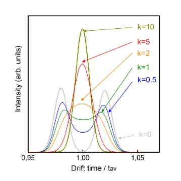
The ability of the above model to generate drift time distributions for different interconversion regimes is illustrated in Figure 1. ATDs have been simulated for interconversion rates ranging from 0 (no interconversion) to 10 times the inverse average drift time. For simplicity, we considered k_AB= k_BA= k with equal initial populations in states A and B. Cases where such conditions are not fulfilled are considered in the next section for reproducing experimental data. The width of the peaks was calculated for a resolution of 70. In the trivial case k = 0, the simulated ATD simply corresponds to the superposition of two Gaussian curves centered around tA and tB. Yet when k is half of the

inverse average drift time, most ions display a drift time intermediate between tA and tB, due to

interconversion. This contribution continuously increases for higher rates, until the probability of no interconversion during the drift becomes negligible. In this case (e.g. k=2, in Figure 1) the ATD consists in a single broad peak centered at a drift time 𝜏0=1₂(tA+ tB) . As k increases further, the

width of the peak decreases until it reaches the resolution-limited width (in the present case for k≈10). Once this high-rate-limit is reached, the case of two interconverting isomers becomes indistinguishable from that of a single static isomer with intermediate drift time.

Beyond the above illustrative results, two important quantities can be derived from the model: the position of the single peak in the high-rate-limit (the above expression only holds in the special case k_AB= k_BA), and an estimate of the maximum transition rate that yields a visible signature in the ATD, i.e. the threshold for the high-rate-limit. To this end, the expansion of the probability functions of equation (12) in the case of high values of kAB and kBA can be used. As demonstrated in the

Supporting Information section (p. S-2), in the limit of high values of the transition rates, the total probability distribution for an arrival time 𝜏 around the time 𝜏0 varies like a Gaussian function whose

full width at half maximum (FWHM) ∆ can be estimated by: ∆= 2√ln (2)tB− tA

8

where 𝑡̅ =1₂(tA+ tB) and 𝑘̅ =1₂(kAB+ kBA). Under the same assumptions, the central value of the

distribution 𝜏0 is:

𝜏₀=xBtB− xAtA

x_B+ x_A (16)

with xA = kABtA and xB = kBAtB.

Based on equation (15), a criterion can be established for the existence of a signature of interconversion on the shape of the ATD. Such signature is visible if ∆ is larger than the peak width expected from the resolution of the instrument. For example, in the case of a drift tube where the resolution is limited by diffusion,9 the effects of interconversion are discernible as soon as the following condition is fulfilled:

tB− tA

𝑡̅ > √2𝑘̅𝑡̅√ 𝑘B𝑇

𝑞𝑉 (17)

where 𝑉is the drift voltage.

Note that similar expressions could be derived in other cases, e.g. for a travelling wave instrument, provided that a good estimate of the expected peak width is available.19

Tandem-IMS measurements

The ATD measured for the singly-charged silver-bound dimer [2Z1+Ag]+ (m/z 667) of the cyclic Z1 azobenzene depicted in Scheme 1 is plotted on the top panel of Figure 2. This distribution is clearly bimodal with a first peak (peak A) centered at tA = 26.0 ms and a second peak (peak B) at tB =28.9 ms.

The intensity in the region intermediate between the two peaks cannot be attributed to the overlap of the distributions (based on the instrumental resolution, the peaks would be nearly baseline-resolved under the experimental conditions).

We then performed tandem-IMS measurements. Namely, after a first IMS separation, only the ions reaching the end of the drift tube within a narrow drift time range were selected and transferred to the middle ion funnel assembly of our instruments, were they could be trapped for a controlled amount of time before injection in a second drift tube. We used a selection window of 1 ms. The ATDs reported in Figure 2 refer to arrival times after injection in the second tube, and correspond to different delays between selection and injection. The radiofrequency field on the ion funnel-trap was shut down for 5 ms between each measurement cycle to ensure that the trap was fully emptied. Figure 2 displays ATDs recorded after selection of peak B. The shortest possible delay achievable between selection and injection in the second tube is limited by the transfer time through the funnel assembly (in this case 4 ms). The corresponding ATD does not consist in a single peak. Although the distribution is dominated by a peak at tB (corresponding to the selection window), a tail at shorter

drift times extending to tA is also visible, indicating that conversion has occurred after selection. As

the time lag 𝛿𝑡𝑟𝑎𝑝 between selection and injection is increased, a second peak at the arrival time tA

appears and grows until it reaches an intensity comparable to that of the peak at tB for 𝛿𝑡𝑟𝑎𝑝 >

100 ms. Such behavior can be attributed to spontaneous interconversion of the Z1-silver-dimer from one form “state B” to another form “state A” that occurs on a timescale of few ten milliseconds. Interestingly, similar results were observed when selecting peak A (Figure S-1): a peak at time tB was

9

Characterization of the interconversion dynamics

Based on the above results, we concluded that A ↔ B isomerization can spontaneously occur under the experimental condition, and that the isomerization rates in both directions are on the same order of magnitude as the inverse drift time. The present system is then a good candidate to test the model described in the previous section. Simulated ATDs were generated based on equation (14) using a numerical integration procedure (Trapezoidal rule). Since the times tA and time tB could be

determined directly from the experiments, the conversion rates kAB and kBA were the only two

unknown parameters for calculating the probabilities in equation (12). We used a Simplex algorithm20 to determine the set of kAB and kBA values that provide the best fit on all ATDs obtained

at different trapping delays. To this end, the initial populations denoted A0 and B0 in equation (14)

were calculated from the rate equations based on trial values for kAB and kBA. We assumed only one

type of isomer was present just after selection. In the case of selection of B ions, with a trapping time 𝛿_{𝑡𝑟𝑎𝑝}, this yields: { A₀ = kBA kBA+ kAB(1 − e −(kBA+kAB)𝛿𝑡𝑟𝑎𝑝₎ B₀= e−(kBA+kAB)𝛿𝑡𝑟𝑎𝑝+ kAB k_BA+ k_AB(1 − e−(kBA+kAB)𝛿𝑡𝑟𝑎𝑝) (18)

The simulated ATDs obtained with the best fitting values kAB=15.2±0.8 s-1 and kBA=12.5±0.8 s-1 are

plotted on top of the experimental ATDs on Figure 2 (and on Figure S-1 ). These values correspond to an average conversion rate of about twice the inverse average drift time.

Temperature-dependent dynamics

The above-described procedure allows determination of kinetic rate constants for a structural transition. In the frame of the transition state theory, the evolution of such rate 𝑘 with temperature is related to the Arrhenius activation energy 𝐸𝐴 for the transition:

𝑘(𝑇) > 𝐴e−𝐸𝐴⁄𝑘B𝑇 (19)

We applied the above procedure to ATDs recorded at different temperatures by thermalizing the chamber housing the drift tubes (the corresponding experimental and simulated ATDs are provided in Figures S-2 and S-3). The current configuration of our instrument only allowed exploring a limited temperature range around room temperature. This was nevertheless sufficient to observe significant changes in the interconversion rates. The values determined for (kAB, kBA) were (9.4±0.5 s-1,

8.6±0.5 s-1), and (35±1 s-1, 27±1 s-1) at 287 K, and 312 K, respectively (the error bars are estimated from the standard deviation of the fit). They are reported on the Arrhenius plot in Figure 3. Activation energies were then extracted from a linear fit, which yields 0.35±0.02 eV for the transition A → B, and 0.40±0.01 eV for B → A.

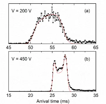
The higher transition rates observed when increasing the temperature also provides an opportunity to test our model in cases where the contribution of interconversion dominates the shape of the ATD. We recorded ATDs at 312 K at different drift voltages V, thus varying the average drift time of the ions, and then the probability for interconversion of the Z1-silver-dimer during the drift. Figure 4 displays ATDs recorded without IMS selection at V=450 V, and 200 V, corresponding to average drift times of 27 ms, and 55 ms, respectively. Since this modification of the drift voltage is not expected to

10

affect the transition rates, this allows exploring different ratios between the transition rate and the inverse drift time, varying from about 1 at V=450 V, to about 2 at V=200 V. The ATDs simulated for the different cases using the same values for kAB and kBA that those previously determined are

plotted together with the experimental profiles on Figure 4. The model reproduces the transition from a bimodal distribution to a broad featureless distribution, related to the dominance of interconversion. The small deviation observed on the profile at 450 V (Figure 4.b) may be attributed to the contribution of minor intermediate conformers between A and B. It can be noted that the distributions obtained at long trapping times does not exactly match the one observed without mobility selection. This supports the hypothesis that if minor isomers are present, they seem not be populated during the interconversion between A and B.

Interpretation of travelling wave data

Beyond the measurement of kinetic constants or activation energies, a more general application of the present model concerns the interpretation of IMS data, especially regarding peak width. The width of the ATDs recorded using travelling wave (TW) instruments remains under-exploited.

The ATDs in Figure 5.a were obtained using a travelling wave (TW) instrument (Synapt G2-Si HDMS, Waters) for the above-discussed Z1-silver-dimer, as well as for the silver-bound dimer from the other form Z2 of the azobenzene represented on Scheme 1. The corresponding ATDs recorded using the drift tube are represented in Figure 5.b. The ATDs recorded with the two instruments for the Z1-silver-dimer are strikingly different. While two peaks are clearly distinguishable in the drift tube ATD, only one broad spectral feature is visible in the TW-ATD. Even if theoretical peak widths are difficult to estimate using a TW instrument, this difference cannot be fully attributed to instrumental resolutions. We will show that interconversion dynamics can account for the observations.

One empirical way to detect abnormally broad spectral features in TW data is to compare peak width for similar species. From the drift tube data, the width of the ATD recorded for the Z2- silver-dimer is compatible with the presence of a single isomer. We then took the TW-ATD of the same Z2- silver-dimer as a reference for the expected peak width under the experimental conditions in the TW instrument. Under this hypothesis, the width of the TW-ATD for the Z1-silver-dimer is clearly broader than expected. From this sole observation one could conclude to the coexistence of several isomers for the Z1- silver-dimer. From the above model, we can propose further interpretation in terms of dynamics. A first estimation of the average interconversion rates in the TW conditions is possible to extract using equation (15), assuming that the ratio tB−t_𝑡̅ A is the same as for the drift tube ATD. Then, based on the experimental width of the TW-ATD, ∆ = 0.87 ms, one can estimate the average transition rate to be 𝑘̅ ≈ 35 s-1.

In the present case, the fitting procedure used for the drift tube spectra is not possible to apply directly to the TW data, since no direct measurement of the drift times tA and tB is available. We

then estimated those values based on the drift tube measurements. Assuming that the ratio between tA or tB and the drift time measured for the Z2-silver-dimer is instrument independent, we

estimated the corresponding TW values 𝑡A𝑇𝑊 ≈ 7.3 ms and 𝑡B𝑇𝑊 ≈ 8.1 ms. The TW-ATD can finally be

reasonably reproduced by the simulation represented in Figure 5 using the following transition rates: k_AB= 388 s-1

, kBA= 272 s-1, and slightly adjusted values for the drift times: 𝑡A𝑇𝑊≈ 7.4 ms and

𝑡_B𝑇𝑊_{≈ 8.4 ms. The width of the Gaussian function used for the convolution was taken to yield a}

11

were assumed to be the stationary ones calculated on the same basis as equation (18). The resulting values are in agreement with the estimate of the average transition rate from the sole peak width. From an extrapolation of our temperature-dependent measurements, the above-estimated rates would correspond to an effective temperature of the ions in the travelling-wave cell of about 370 K. The order of magnitude of the increase in temperature due to RF confinement is more important than the slight change recently reported by Allen and Bush using similar hardware.21 It is however smaller than the values measured by Morsa et al.,14 or Merenbloom et al..15

Conclusions

An analytical model was proposed that accounts for the influence of interconversion dynamics on the shape of the arrival time distributions recorded using ion mobility instruments. This model was able to reproduce experimental data for a bi-stable system and allowed to extract rate constants for the observed structural transitions, based on tandem-IMS measurements. In addition, we show that the proposed procedure also enables determination of activation energies through temperature-dependent experiments. Finally, we use our model to interpret differences in experimental data obtained from different instruments in terms of conformational dynamics.

The present results open the possibility to extend the application range for conformational dynamics studies using IMS, and especially tandem-IMS. Moreover the proposed model is a straightforward tool to interpret IMS data in cases where dynamics may play a role. It could be of particular interest in the frame of emerging uses of IMS that rely on the observation of structural transitions induced by collisions,22 charge-transfer reactions,23 temperature changes,24 and irradiation by light.25–27 More generally, from the comparison between drift tube and travelling-wave measurements on the same system, we showed that dramatic differences can arise from different experimental conditions, due to the sensitivity of conformational dynamics to ion temperature.

The above example illustrates that interconversion dynamics should be considered when discussing the shape of the peaks in ATDs to avoid possible errors in structural interpretation. Moreover, interconversion dynamics may be a pitfall in the use of IMS databases, since it could limit the possibility to compare results obtained from different instruments, or using different instrument conditions. This is particularly critical when using radiofrequency-based devices, where substantial collision activation may occur depending on the conditions.14,21,15

Acknowledgements

The research leading to these results has received funding from the European Research Council under the European Union’s Seventh Framework Program (FP7/2007-2013 Grant Agreement No. 320659). The post-doctoral fellowship to S.P. has been supported by the ANR CHARMMMAT (ANR-11-LABX-0039).

12

References

(1) Trimpin, S.; Clemmer, D. E. Anal. Chem. 2008, 80 (23), 9073–9083.

(2) Fernandez-Lima, F. A.; Becker, C.; McKenna, A. M.; Rodgers, R. P.; Marshall, A. G.; Russell, D. H. Anal. Chem. 2009, 81 (24), 9941–9947.

(3) Jarrold, M. F. Phys. Chem. Chem. Phys. 2007, 9, 1659–1671.

(4) Baker, E. S.; Bernstein, S. L.; Bowers, M. T. J. Am. Soc. Mass Spectrom. 2005, 16 (7), 989– 997.

(5) Pierson, N. A.; Chen, L.; Russell, D. H.; Clemmer, D. E. J. Am. Chem. Soc. 2013, 135 (8), 3186–3192.

(6) Albrieux, F.; Ben Hamidane, H.; Calvo, F.; Chirot, F.; Tsybin, Y. O.; Antoine, R.; Lemoine, J.; Dugourd, P. J. Phys. Chem. A 2011, 115 (18), 4711–4718.

(7) Marklund, E. G.; Degiacomi, M. T.; Robinson, C. V.; Baldwin, A. J.; Benesch, J. L. P. Structure 2015, 23 (4), 791–799.

(8) Uetrecht, C.; Barbu, I. M.; Shoemaker, G. K.; van Duijn, E.; HeckAlbert J. R. Nat. Chem. 2011,

3 (2), 126–132.

(9) Revercomb, H. E.; Mason, E. A. Anal. Chem. 1975, 47 (7), 970–983.

(10) Hudgins, R. R.; Dugourd, P.; Tenenbaum, J. M.; Jarrold, M. F. Phys. Rev. Lett. 1997, 78 (22), 4213–4216.

(11) Gidden, J.; Bushnell, J. E.; Bowers, M. T. J. Am. Chem. Soc. 2001, 123 (23), 5610–5611.

(12) Kaleta, D. T.; Jarrold, M. F. J. Am. Chem. Soc. 2003, 125 (24), 7186–7187.

(13) Wyttenbach, T.; Pierson, N. A.; Clemmer, D. E.; Bowers, M. T. Annu. Rev. Phys. Chem. 2014,

65, 175–196.

13

(15) Merenbloom, S. I.; Flick, T. G.; Williams, E. R. J. Am. Soc. Mass Spectrom. 2012, 23 (3), 553– 562.

(16) Simon, A.-L.; Chirot, F.; Choi, C. M.; Clavier, C.; Barbaire, M.; Maurelli, J.; Dagany, X.; MacAleese, L.; Dugourd, P. Rev. Sci. Instrum. 2015, 86 (9), 94101.

(17) Deo, C.; Bogliotti, N.; Métivier, R.; Retailleau, P.; Xie, J. Chem. - A Eur. J. 2016, 22 (27), 9092–9096.

(18) Giddings, J. C.; Eyring, H. J. Phys. Chem. 1955, 59, 416–421.

(19) Kune, C.; Far, J.; De Pauw, E. Anal. Chem. 2016, 88 (23), 11639–11646.

(20) Press, W. H.; Teukolsky, S. A.; Vetterling, W. T.; Flannery, B. P. In Numerical Recipes in C

(Second edition); Cambridge University Press: Cambridge, 1992; pp 408–412.

(21) Allen, S. J.; Bush, M. F. J. Am. Soc. Mass Spectrom. 2016, 27 (12), 2054–2063.

(22) Tian, Y.; Han, L.; Buckner, A. C.; Ruotolo, B. T. Anal. Chem. 2015, 87 (22), 11509–11515.

(23) Laszlo, K. J.; Munger, E. B.; Bush, M. F. J. Am. Chem. Soc. 2016, 138 (30).

(24) Dickinson, E. R.; Jurneczko, E.; Pacholarz, K. J.; Clarke, D. J.; Reeves, M.; Ball, K. L.; Hupp, T.; Campopiano, D.; Nikolova, P. V.; Barran, P. E. Anal. Chem. 2015, 87 (6).

(25) Markworth, P. B.; Adamson, B. D.; Coughlan, N. J. A.; Goerigk, L.; Bieske, E. J. Phys. Chem.

Chem. Phys. 2015, 17 (39), 25676–25688.

(26) Czerwinska, I.; Kulesza, A.; Choi, C.; Chirot, F.; Simon, A.-L.; Far, J.; Kune, C.; de Pauw, E.; Dugourd, P. Phys. Chem. Chem. Phys. 2016, 18 (47), 32331–32336.

(27) Choi, C. M.; Simon, A.-L.; Chirot, F.; Kulesza, A.; Knight, G.; Daly, S.; MacAleese, L.; Antoine, R.; Dugourd, P. J. Phys. Chem. B 2016, 120 (4), 709–714.

14

Figure 1 : ATDs simulated based on equation (14) assuming kAB= kBA= k and 𝐴0= 𝐵0 = 1. k is

expressed in units of the inverse average drift time. For k = 10, the distribution is indistinguishable from the expected diffusion-limited ATD centered at time tav.

15

Figure 2: (Black squares) ATDs recorded for the Ag-bound Z1-azobenzene dimer. Drift conditions: 4.0 Torr Helium at 297 K, drift voltage 450 V. (a) without mobility selection, (b-d) after selecting peak B and trapping for different durations, (Red Lines) Simulated ATD with values for the transition rates fitted on all datasets recorded at the same temperature.

16

Figure 3: Arrhenius plot based on the values determined for kAB (black squares) and kBA (red circles)

at different temperatures. The solid lines correspond to linear fits on the data.

Figure 4: (Black squares) ATDs recorded for the Ag-bound Z1-azobenzene dimer. Drift conditions: 4.0 Torr Helium at 312 K, at different drift voltages (a) V=200 V, (b) V=450 V. (Red Lines) Simulated ATD with values for the transition rates fitted on all datasets recorded at the same temperature.

17

Figure 5: ATDs recorded for the Ag-bound azobenzene dimer using (a) a travelling wave instrument or (b) a drift tube instrument. (Black squares) Z1 form. (Grey circle) Z2 form shown for comparison. (Red Line) ATD simulated for the Z1 form (see text for details). (Grey line) ATD simulated for the Z2 form considering a single isomer and diffusion-limited resolution. Drift conditions for TW: wave velocity 800 m.s−1, wave height 40 V and N2 gas flow adjusted at 90 mL.min−1 (3.09 mbar). ATDs

recorded for the Ag-bound azobenzene dimer without IMS selection. Drift conditions for drift tube: 4.0 Torr Helium at 287 K, drift voltage 450 V.