A continuous-wave second harmonic gyrotron oscillator at 460 GHz

A Continuous-Wave Second Harmonic Gyrotron

Oscillator at 460 GHz

by

Melissa Kristen Hornstein

B.S., Rutgers University (1999)

S.M., Massachusetts Institute of Technology (2001)

Submitted to the Department of Electrical Engineering and Computer

Science

in partial fulfillment of the requirements for the degree of

Doctor of Philosophy

at the

MASSACHUSETTS INSTITUTE OF TECHNOLOGY

June 2005

©

_{Massachusetts Institute of Technology 2005. All rights reserved.}

Author...

... ,...

.

...

Department of Electrical Engineering and Computer Science

May 16, 2005

Certified by...

... /...

Richard J. Temkin

Senior Research Scientist, Department of Physics

~~

Thesis

Supervisor

Accepted by ...

Arthur C. Smith

Chairman, Department Committee on Graduate Students

OF TECHNOLOGY

IOCT

2 1 2005

A Continuous-Wave Second Harmonic Gyrotron Oscillator

at 460 GHz

by

Melissa Kristen Hornstein

Submitted to the Department of Electrical Engineering and Computer Science on May 16, 2005, in partial fulfillment of the

requirements for the degree of Doctor of Philosophy

Abstract

We report the short pulse and CW operation of a 460 GHz gyrotron oscillator both at the fundamental (near 230 GHz) and second harmonic (near 460 GHz) of electron cyclotron resonance. During operation in a complete CW regime with 12.4 kV beam voltage and 135 mA beam current, the gyrotron generates a record 8 W of power in

the second harmonic TEO,₆,1 mode at 458.6 GHz. Design at high frequency, second

harmonic, and low beam power is challenging because the latter two involve lower

gain than at fundamental modes and all three necessitate higher

Q

complete computer control, the gyrotron has stably operated continuously for over an hour near 460 GHz. Diagnostic radiation pattern measurements of the beam using an array of pyroelectric sensors show a bi-Gaussian beam with 4% ellipticity. Operation

in the fundamental modes, including the TEO,3,1 mode at 237.91 GHz and the TE₂,₃,₁

at 233.15 GHz, is observed at peak output powers up to 70 W. CW studies of the

fundamental TE2,3 mode at low voltage reveal that the mode can be excited with less

than 7 W of beam power at less than 3.5 kV. Further, we demonstrate broadband continuous frequency tuning of the fundamental modes of the oscillator over a range of more than 2 GHz through variation of the magnetic field alone. We interpret these results in terms of smooth transitions between higher order axial modes of the resonator.

In a related experiment, second harmonic (in addition to fundamental) operation of a nominally 250 GHz gyrotron oscillator was characterized to verify the possibility of second harmonic excitation at 460 GHz. The characterization experiments yielded results of extremely low second harmonic start oscillation currents, as low as 12 mA,

and have been interpreted as an unintentionally high

Q

stable CW source, the 250 GHz gyrotron was the first gyro-device specifically designed with the purpose of seamless integration into an NMR spectrometer. Under complete computer control, the gyrotron's operation for over 10 days has been observed, yield-ing a power stability of better than 1% and frequency stability of better than 400 Hz. Overmoded corrugated waveguide was designed and implemented to enable low loss quasi-(Gaussian transmission. In conjunction with the corrugated waveguide, a quasi-optical directional coupler was designed and implemented to enable feedback

on the forward (and reflected) power to further stabilize the signal.

Radiation intensity patterns were compared using four techniques: thermal paper, liquid crystal paper, an array of pyroelectric sensors, and a mechanized scanner. The liquid crystalline technique was adapted from a technique employed in temperature measurements in electronic devices. Originally employed for use in diagnosing laser beams, we demonstrate the first use of a pyroelectric camera at millimeter frequencies.

A study of the overmoded microwave transmission and mode conversion system

of a 140 GHz gyrotron oscillator, the first in a series of DNP gyrotrons, is also presented. The losses were characterized under a succession of iterative configurations for optimization of power transmission, including the design and implementation of a new TEO,1 to TE1,1 waveguide mode converter. The result of this study was a

reduction of the total loss of the transmission system from nearly 9 dB to 4.5 dB. In addition to becoming a milestone in high frequency second harmonic design, the successful completion of the 460 GHz gyrotron experiment will allow the highest field

DNP experiments to date. The success of experiments on three gyrotron oscillators, at

460, 250, and 140 GHz makes an important contribution to the body of knowledge on the development of high frequency, CW, second harmonic, and low power gyrotrons. Thesis Supervisor: Richard J. Temkin

Acknowledgments

I would like to acknowledge my thesis supervisor Richard Temkin; my first supervisor

Kenneth Kreischer for accepting me on to the project; Director of the Francis Bit-ter Magnet Laboratory Professor Robert Griffin; Vikram Bajaj of the Griffin Group for our many collaborations on DNP and gyrotrons at 250 and 460 GHz, teaching me about NMR and DNP; my thesis committee, Professors Qing Hu and Ronald Parker; Professor Jin Au Kong, my academic advisor; Ivan Mastovsky for the tech-nical aspects of my experiment, including drawing and assembling the components of the tube, William Mulligan for electrical assistance including power supplies and the high voltage modulator; Paul Woskov (Associate Head, Plasma Technology and Systems Division) for our collaborations at 250 GHz; Michael Shapiro, Head of the Gyrotron Group, for theoretical assistance; Jeffrey Bryant, Ajay Thakkar, Ronald DeRocher, Peter Allen, and Michael Mullins of the Francis Bitter Magnet Labora-tory for technical and machining assistance; Catherine Fiore and Amanda Hubbard of the Plasma Science and Fusion Center; Robert Childs for the use of his boro-scope in troubleshooting my experiment and for his knowledge on vacuum systems and William Byford for electrical assistance, both of the Plasma Science and Fusion Center; John Machuzak, James Anderson, Jagadishwar Sirigiri, Stephen Korbly, and Jeffrey Vieregg of the Gyrotron Group; Melanie Rosay, Kan-Nian Hu, and Volker Weis of the Griffin Group; Alexander Vlasov of the University of Maryland and SAIC for elucidating MAGY.

Contents

1 Introduction

1.1 Terahertz . . . .

1.1.1 State-of-the-art . . . . .

1.1.2 Interactions with matter

1.2 Cyclotron Resonance Masers

1.2.1 Harmonic considerations

1.2.2 History . . . .

1.2.3 Operating Principles . .

1.2.4 State-of-the-art . . . . .

1.3 Dynamic Nuclear Polarization .

1.4 Thesis Outline . . . . 2 Theory 2.1 Introduction . . . . 2.2 CRM Interaction . . . . 2.2.1 Harmonic CRM Interaction . . . . . 2.3 Kinetic Theory . . . .

2.3.1 Linearized Dispersion Relation . . . .

2.4 Single-Particle Theory . . . .

2.4.1 Start Oscillation Current . . . .

2.4.2 Ohmic Losses . . . .

2.5 Quantum Mechanical Basis of the Cyclotron

2.6 Waveguide Theory . . . .

2.7 Numerical Methods . . . .

2.7.1 _{Cold Cavity . . . .}

2.7.2 Starting Current Calculation Includin

Resonance Mas

g Beam Effects 2.7.3 _{MAGY . . . .}

2.7.4 _{E G U N . . . .}

2.8 _{Sensitivity-Enhanced Nuclear Magnetic Resonance . . . .}

27 . . . . 2 7 . . . . 2 7 . . . . 2 9 . . . . 3 0 . . . . 3 1 . . . . 3 2 . . . . 3 2 . . . . 3 3 . . . . 3 4 . . . . 3 5 37 37 38 40 42 43 46 49 50 51 55 57 58 60 61 63 64 er

2.8.1 Chemical Shift . . . . 2.8.2 Nuclear Magnetic Resonance in the Solid State

2.8.3 Dynamic Nuclear Polarization . . . .

2.9 D iscussion . . . .

3 Experimental Setup and Diagnostics

3.1 D iagnostics . . . .

3.1.1 High Frequency Detection . . . .

3.1.2 Power Measurement . . . . 3.1.3 Radiation Pattern Measurement . . . .

3.1.4 Time-Domain Signal Measurement . . . .

3.1.5 Vacuum Diagnostics . . . . 3.1.6 Thermal Load Measurement . . . .

3.1.7 Small-Signal Detection . . . .

3.1.8 Cold Test . . . .

3.2 Equipm ent . . . .

3.2.1 Pulsed Equipment . . . . 3.2.2 CW Equipment . . . .

4 Design of a 460 GHz Second Harmonic

4.1 Target Specifications . . . .

4.1.1 Dynamic Nuclear Polarization .

4.2 Second Harmonic Considerations . . .

4.2.1 Mode Competition . . . .

4.2.2 Start Oscillation Current . . . .

4.2.3 Ohmic Losses . . . .

4.3 Components . . . .

4.3.1 Electron Gun . . . .

4.3.2 Magnet System . . . .

4.3.3 Interaction Structure . . . .

4.3.4 Quasi-Optical Mode Converter .

4.3.5 Vacuum System . . . .

4.3.6 Vacuum Output Window . . . .

4.3.7 Collector . . . . 4.4 Control System . . . . 4.4.1 Software . . . . 4.4.2 Interlocks . . . . 4.5 Discussion . . . . Gyrotron Oscillator . . . . . . . . . . . . . . . . . . . . . . . . . . . . .-. .-. .-. .-. .-. .-. .-. .-. .-. .-. .-. .-. .-. . . . . . . . . . . . . . . . . . . . . . . . . . . . . . . . . . . . . . . . . . . . . 65 . . . . 66 . . . . 67 . . . . 68 69 . . . . 69 . . . . 69 . . . . 73 . . . . 75 . . . . 77 . . . . 79 . . . . 83 . . . . 85 . . . . 86 . . . . 87 . . . . 87 . . . . 90 91 91 91 95 95 97 99 100 100 106 111 112 114 115 116 118 118 121 121

5 460 GHz Second Harmonic Experiments

5.1 Short Pulse Experiment [1] ...

5.1.1 M ode M ap .. .. .... ... .. ... ...

5. [.2 Start Oscillation Current . . . .

5.1.3 Second Harmonic . . . .

5. 1.4 Power in Fundamental TEO,3 Mode . . . . . 5.1.5 Broadband Continuous Frequency Tuning

5.2 CW Experiment . . . . 5.2.1 M ode M ap . . . . 5.2.2 Second Harmonic . . . . 5.2.3 Frequency Pulling . . . . 5.2.4 Ohmic Losses . . . . 5.2.5 Homodyne Measurements . . . . 5.2.6 Low Voltage Fundamental TE₂,₃ Mode . . .

5.2.7 Hollow Dielectric Waveguide . . . . 5.2.8 Radiation Patterns . . . .

5.2.9 Stability . . . .

5.3 Low Power

Q

5.4 D iscussion . . . .

6 250 GHz Gyrotron Experiments

6. 1 Characterization of the 250 GHz Gyrotron

6. 1.1 TEO,3 Operating Mode . . . . 6.1.2 Frequency Pulling . . . .

6.1.3 Radiation Patterns . . . .

6.1.4 CW Long-term Stability and Control .

6.1.5 Linewidth . . . .

6.2 Low Second Harmonic Starting Currents . . .

6.3 Corrugated Waveguide and Directional Coupler

6.3.1 Introduction . . . .

6.3.2 Component Design . . . .

6.3.3 Cold Tests . . . .

6.3.4 Measurements with Gyrotron . . . . .

6.3.5 Conclusions . . . . 6.4 D iscussion . . . . Experiment 123 123 125 127 130 132 136 141 145 146 147 149 155 156 161 167 168 169 174 177 178 179 181 182 187 188 190 200 200 201 207 210 214 215

[2]

7 Transmission System of a 140 GHz Gyrotron Oscillator

7.1 Two-Dimensional Radiation Pattern Measurements . . . .

7.1.1 Gyrotron Radiation Pattern Measurements . . . .

7.1.2 Old Mode Converter Radiation Pattern Measurements 7.1.3 New Mode Converter Radiation Pattern Measurements

7.2 Modifications to the 140 GHz Transmission System . . . .

7.2.1 Design of a New TEO,1-TE1,1 Waveguide Mode Converter 7.2.2 Overmoded Miter Bend Near Probe . . . .

7.2.3 Oblique Gyrotron Beam . . . .

7.2.4 B eat . . . . 7.2.5 Corrugated Waveguide . . . .

7.2.6 Theoretical Transmission Line Losses . . . .

7.2.7 Summary of Experimental Losses . . . .

7.3 Summary and Discussion . . . .

8 Conclusions

8.1 460 GHz Second Harmonic Gyrotron Oscillator

8.2 250 GHz Gyrotron Oscillator Experiments . . .

8.3 140 GHz Gyrotron Oscillator Experiments . . .

8.4 Gyrotron Comparisons . . . . 8.4.1 Frequency Pulling . . . . 8.4.2 Radiation Patterns . . . . 8.5 Future W ork . . . . 249 . . . . 249 . . . . 250 . . . . 251 . . . . 252 . . . . 252 . . . . 252 . . . . 253 217 . . . 220 . . . 220 . . . 226 . . . 229 . . . 235 . . . 235 . . . 238 . . . 239 . . . 240 . . . 240 . . . 242 . . . 245 . . . 245

List of Figures

1-1 State of the art in CW terahertz sources. . . . . 28

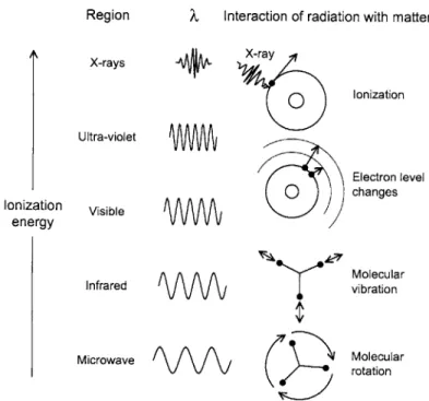
1-2 The interactions of the bands of the electromagnetic spectrum with

m atter. . . . . 29

1-3 (a) Typical gyrotron oscillator cavity with electron beam, (b) RF field

profile with single axial maximum, (c) phase, and (d) applied DC

mag-netic field . . . . 33

2-1 Simulation of a non-uniform electron phase distribution which occurs

due to the interaction of a relativistic electron beam with a transverse electric field E, situated in a static magnetic field BO. The beamlets, with Larmor radius rL, represent snapshots in phase space in both

axial locations throughghout the interaction structure (from z = 0 to

z _{:= L) and tim e [3] . . . . 39}

2-2 Cross-section of the beam geometry in the interaction region of a

cylin-drical resonant gyrotron cavity operating in the TEO,, mode for (a) ini-tial random phasing of electrons in their cyclotron orbits (b) electrons

bunched in phase in their cyclotron orbits. . . . . 40

2-3 Electron motion for resonance at (a) second and (b) third cyclotron

harmonics. The solid line shows the initial trajectory of electrons and

the electric field is represented by dashed lines. Adapted from [4]. . . 42

2-4 _{Dispersion diagram of a gyrotron oscillator showing the region of}

in-teraction between the fast waveguide mode and the beam cyclotron modes. (a) Fundamental beam cyclotron mode and waveguide mode intersect at fundamental resonance. The dots represent the longitu-dinal cavity modes. The intersection of the beam cyclotron modes with waveguide modes at negative values of k2 causes the excitation of backward wave oscillations. (b) The intersection of the third harmonic of the cyclotron mode with the waveguide mode gives rise to a third

n hQ2

2-5 Cyclotron resonance for varying values of the parameter k C

according to equation (2.84), where terms of order (hQc/moc) 2 have

been neglected. Note that a completely absorptive line is recovered in

the non-relativistic lim it. . . . . 54

2-6 Intensity patterns of the five lowest order transverse electric (TE)

waveguide modes; (a) TE1,1, (b) TE2,1, (c) TEo,1, (d) TE3,1, and (e)

T E 4,1. . . . .

58

2-7 Operating frequency shift with reference frequency offset. The

conver-gent solution is located at the origin. . . . . 61

3-1 Block diagram of a heterodyne receiver used as a millimeter and

sub-millimeter wavelength frequency measurement system. . . . . 70

3-2 Insertion loss of the IF and LO from the diplexer (Pacific Millimeter

Products, Model No. MD5, S/N 008). The IF band is flat from DC to 12 GHz and the LO band is flat over 20 to 40 GHz [5]. . . . . 71

3-3 Photograph of the frequency system, picturing the oscilloscope,

fre-quency counter, and power supply on the right, and the local oscillator, amplifiers, and filter on the left (inside the boxes). The horn, mixer,

and attenuator are not depicted. . . . . 71

3-4 Intermediate frequency signal for the second harmonic TE2,6,1 mode at

456 GHz using the frequency measurement system. . . . . 72

3-5 Reflectivity of the laser calorimeter, as measured by a dispersive Fourier

transform spectrometer [6, 7]. . . . . 73

3-6 Block diagram of near- and far-field scanner. . . . . 75

3-7 Typical time-domain diode signal of the TEO,3,1 mode at the voltage

and current shown in Figures 3-14 and 3-8 and 8.58 T. . . . . 77

3-8 Typical collector and body current signals using a Rogowoski current

monitor. The corresponding voltage pulse is shown in Fig. 3-14. The

signal corresponds to the TE,3,1 mode at 8.58 T, and the diode trace

shown in Figure 3-7. . . . . 78

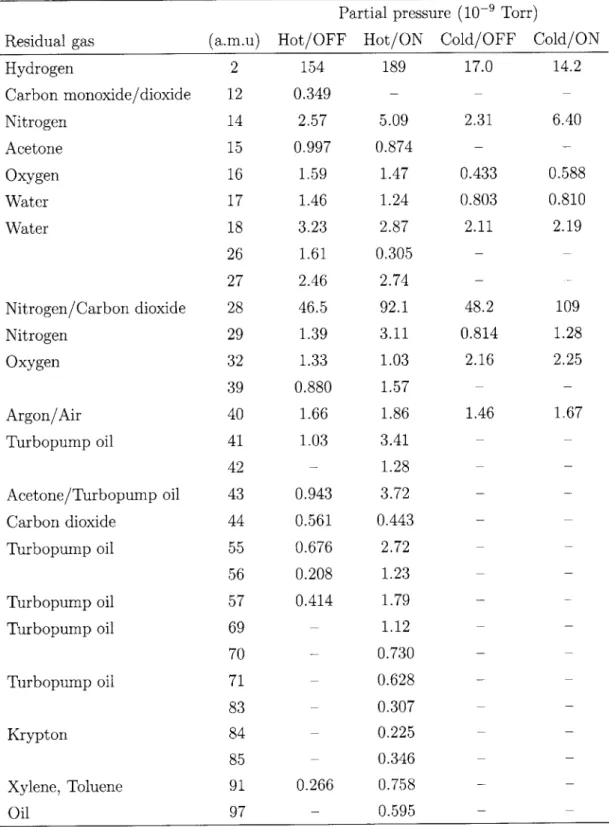
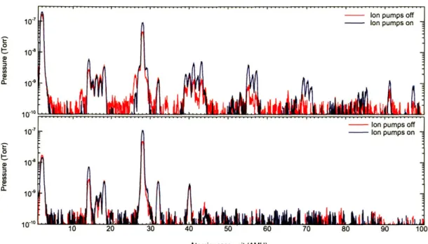
3-9 Typical RGA traces at the end of a bakeout when the tube is at 100'C

(top) and room temperature (bottom). . . . . 81

3-10 Relationship between the current drawn from 8 L/s Varian-style ion

pumps operated at 3.5 kV and the vacuum pressure in Torr. . . . . . 83

3-11 Thermistor resistance measuring circuit. . . . . 85 3-12 Far-field radiation scan of the cylindrical TE1,1 output of the BWO at

3-13 Power drift over frequency of the BWO. . . . . 8

3-14 Typical voltage pulse from the high voltage modulator. The corre-sponding current trace is shown in Fig. 3-8. The signal corresponds to

the TEO,3,1 mode at 8.58 T, and the diode trace shown in Figure 3-7. 88

3-15 Calibration of the cathode voltage readout. . . . . 88 3-16 Photograph of (a) the front end of the high voltage modulator (b) the

CW gyrotron console, showing the cryogenic temperature monitors, liquid cryogen level monitor, ion pump controllers, CW switching high voltage power supply, gun coil power supply, computer controls, and

superconducting magnet power supply. . . . . 89

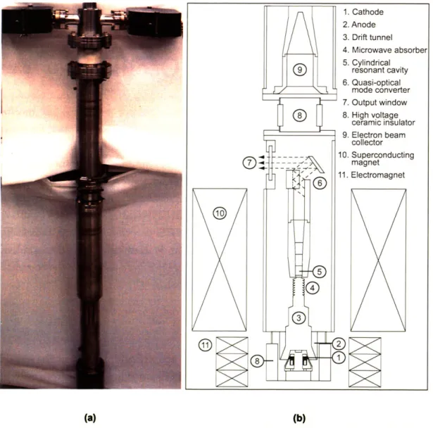
4-1 (a) Photograph of the gyrotron tube free-standing (b) Cross-sectional

schematic of the cylindrically symmetric 460 GHz gyrotron tube, not

shown to scale, indicating key components. . . . . 92

4-2 _{Photograph of the author and the 460 GHz gyrotron located in the}

bore of the superconducting magnet. . . . . 93

4-3 Chart of the TE mode indices up to to Vmp = 30 for the fundamental

modes and vmp = 60 for the second harmonic modes. . . . . 96

4-4 Coupling factor for (a) the TEO,₆ and TE2,6 second harmonic modes of

both rotations and (b) the nearby competing co- and counter-rotating

TB2,3 and TE8,1 fundamental modes. . . . . 96

4-5 _{Starting currents at 12 kV and alpha and spread parameters taken}

from EGUN simulations (c.f. Fig. 4-9). In the case where the alpha

from the EGUN simulation is undefined, an beam alpha of 2.0 and corresponding velocity spread is used. Solid lines represent second

harmonic modes and dotted lines fundamental modes. . . . . 98

4-6 Theoretical RF efficiency in the 460 GHz gyrotron cavity. . . . . 99

4-7 Photographs of the (a) cathode and (b) anode. . . . . 100

4-8 _{(a) Test data on the 460 GHz cathode (Semicon, Model No.}

BGC-10-1 S/N 0001969) by J. Tarter [8] (b) Current-voltage data for various

cathode temperatures. _{. . . . 101}

4-9 (a) _{Velocity pitch factor and (b) transverse velocity spread for the}

low-voltage, diode-type gun used in the 460 GHz gyrotron experiment. Each curve is derived from EGUN simulations of the gun geometry

conducted as a function of voltage and magnetic field. . . . . 102

4-10 Simulation of the evolution of the transverse and axial velocities of the

electrons accelerated at 12 kV in the 460 GHz gyrotron experiment using the EGUN electron optics and gun design program. The simula-tion includes the electron trajectories, equipotential lines, cathode and

anode geometries, and 8.4 T applied magnetic field of the gun region. 103

4-11 (a) Transverse (solid line) and longitudinal (dashed line) electron beam velocity and transverse spread (dotted line) and (b) electron beam

velocity pitch factor predictions by EGUN. . . . . 104

4-12 Millisecond pulse tests of the Spellman high voltage power supply over a 700 kQ resistive load. The red waveforms indicate the high voltage response and the blue lines are the driving pulse shape for pulses of

length (a) 5 ms, (b) 20 ms, (c) 100 ms, and (d) 20 ms. . . . . 105

4-13 Comparison of measured axial field profile (x's) to Cryomagnetics

(solid line) magnetic field profile. . . . . 106

4-14 Superconducting magnet drawings, designed by Cryomagnetics, Inc. [9.107

4-15 Fringe-field plot for the 700 MHz/89 mm superconducting NMR mag-net system (Magnex Scientific, Model No. 700/89-4463) [10]. . . . . .111

4-16 (a) Cross-sectional schematic of the cylindrical 460 GHz gyrotron cav-ity with the axial radiation field profile for the second harmonic TEO,6,1

resonator mode. (b) Intensity pattern of the TEO,6 design mode. . . . 112

4-17 Photograph of the cavity, waveguide, and internal quasi-optical mode converter (launcher, focusing mirror, and steering mirror). The ruler is set at 2 cm and its position approximately corresponds to the location

of the electroformed interaction cavity. . . . . 113

4-18 Schematic of the quasi-optical internal mode converter showing cal-culated design parameters (a) side view (b) front view, adapted from

[11]. . . . .. . .. .. . . .. . . 113

4-19 Transmission of second harmonic and fundamental modes through 1.9990 mm (a) and 1.9736 mm (b) thick Corning 7980 fused silica gyrotron

w indow s. . . . . 115

4-20 Photograph of the window through the cross-bore of the

superconduct-ing magnet. The mode converter is visible. . . . . 116

4-21 Schematic of the collector including the electron beam and water

cool-ing circuit. . . . .. . . . .. 117

4-22 Front panel of the LabVIEW control system. (a) Event driven control

5-1 _{Voltage, diode voltage, collector current, and body current traces of} the TE2,6,1 second harmonic mode at 12.5 kV, 100 mA, and 8.34 T. . 124

5-2 _{Mode map for the design mode and nearby competing fundamental}

TE ₂,3 mode for beam voltage and cavity magnetic field at 100 mA.

The gun coil has been optimized for each point. . . . . 126

5-3 (a) Summary of experimental starting current data (b) measured

fre-quency vs. magnetic field recorded for resonant cavity modes from 5.6 to 9.2 T and up to 15 kV and 160 mA. Open symbols denote

funda-mental modes and filled-in symbols denote second harmonic modes. . 128

5-4 Intensity patterns of the (a) TE2,2, (b) TE4,2, (c) TE2,3, (d) TEO,3, and

(e) TE5,2 fundamental waveguide modes. . . . . 128

5-5 Second harmonic TE2,6,1 and TEO,6,1 start oscillation current data (points)

compared with linear theory (solid lines) at 13.1 kV. . . . . 129

5-6 Intensity patterns of the (a) TE2,6 and (b) TEO,6 second harmonic

waveguide m odes. . . . . 130

5-7 Efficiency of the TE2,6 second harmonic mode at 100 mA (a) as a

function of main magnetic field and (b) as a function of voltage. . . . 131

5-8 Efficiency of the TEO,₆ second harmonic mode at 100 mA (a) as a

function of main magnetic field and (b) as a function of voltage. . . . 132

5-9 Frequency pulling of the (a) TEo,6 and (b) TE2,6 second harmonic modes. 133

5-10 IF signal of 261 MHz with LO frequency of 25.360 GHz at the

eigh-teenth harmonic yields a second harmonic TE2,6 frequency of 456.219

GHz at 8.34 T, 12.5 kV, and 100 mA. . . . 133 5-11 Contour plot of (a) measured peak power data of the fundamental

TFo,3,q modes in watts as a function of beam current and magnetic

field using a pyroelectric detector. The electron gun was pulsed for several microseconds at a repetition rate of approximately 30 Hz with

9 kV. The power level was calibrated using a calorimeter. (b) MAGY

simulated power at experimental conditions. . . . . 134

5-12 Power in the TEO,_{3 mode detected by a laser calorimeter at 9 kV, 100} mA, repetition rate 30 Hz, and pulse length 2.8 pus. These data were

used to calibrate the pyroelectric detector data shown in Fig. 5-11(a). 135

5-13 Mode competition between the TEO,₃ and parasitic TE2,3 fundamental

5-14 (a) Start oscillation currents, (b) frequency tuning, and (c) df/dB nor-malized to the frequency at the minimum start current versus magnetic field normalized to the field at the minimum start current of

fundamen-tal modes from 7.8 to 9.2 T. . . . . 138

5-15 Dispersion diagram showing the region of interaction between the

un-perturbed TE5,2 waveguide dispersion curve and the experimentally

observed Doppler shifted beam cyclotron modes. The intersection of the beam cyclotron modes with the waveguide mode at negative values of k, implies interaction of the beam with a backward propagating wave. 140

5-16 Linear theory (solid circles) and MAGY simulation (solid triangles)

us-ing EGUN calculated parameters of the frequency tunus-ing of the TE5,2,q

modes compared to the experiment (+). The dotted line is the

rela-tivistic cyclotron frequency. . . . . 140

5-17 Linear theory (lines) using EGUN calculated parameters of the

start-ing currents of the TE5,2,q modes compared to the experimental data

(diam onds). . . . . 141 5-18 Self-consistent axial field and phase profiles for TE5,2,q modes with q >

1 as calculated from MAGY. The cavity geometry is indicated above each column, and we have displayed the normalized voltage amplitude.

The frequency increases from 246.0 GHz in (a) to 248.1 GHz in (h). . 142

5-19 Self-consistent axial field profiles for TE5,2,q modes with q > 1 as cal-culated from MAGY (solid lines) compared with cold cavity (dashed lines) and sinusoidal (dotted lines) field profiles. The cavity geometry

is indicated above the column. . . . . 142

5-20 Spatial dependence of the power throughout the cavity (in the TE5,2 mode) at three magnetic fields. At frequencies greater than that of the

TE5,2,1 cold cavity mode, there is a spatial oscillation pattern which we interpret as the interference of the backward propagating wave with its

non-synchronous reflection [12]. . . . . 143

5-21 Mode map for the design mode and nearby competing fundamental

TE2,3 mode at 12.4 kV and 100 mA for the cavity and cathode magnetic

field s . . . . 145 5-22 CW output power measured in the TEO,6 second harmonic mode as a

function of (a) beam current, (b) main magnetic field, (c) voltage, and

(d) cathode magntic field. Unless otherwise indicated, the

5-23 EGUN simulations for varying cathode magnetic fields at 12.4 kV and

100 m A . . . 149

5-24 Frequency tuning of the TEO,6 second harmonic mode with (a) beam

current, (b) main magnetic field, (c) voltage, and (d) cathode magnetic

field. Unless otherwise indicated, the experimental parameters are 12.4 kV, 100 mA and 8.384 T. . . . 150 5-25 Theoretical RF efficiency as a function of the conductivity of copper

and diffractive

Q

calcula-tion assumes alternately a diffractive

Q

conduc-tivity of ideal copper. . . . . 152

5-26 Cavity thermal load and RF efficiency as a function of measured output

power using cavity thermal load measurement for the second harmonic

T Eo,, 1 m ode. . . . 153 5-27 Block diagram of a simple homodyne detector [13]. . . . . 153 5-28 Homodyne measurements of the technical noise for the second

har-monic TEO,6,1 m ode. . . . . 154

5-29 CW output power in the TE2,3 mode as a function of beam current at

3.5 kV and 8.38 T . . . 156

5-30 CW start current data in the TE2,3 mode at 3.5 kV compared to linear

theory using alpha 2.5 and 10% transverse velocity spread. . . . . 157

5-31 CW output power and frequency in the TE2,3 mode as a function of

magnetic field for 50 mA and 3.5 kV. . . . 157 5-32 Contour plot of measured CW power data of the fundamental TE2,₃,q

modes in watts as a function of beam current and magnetic field. . . 158

5-33 Heterodyne measured frequencies of the axial TE2,₃,q fundamental modes

at low voltage as a function of beam current and magnetic field. . . . 159

5-34 (a) Experiment (homodyne) compared to (b) MAGY simulation of the TE2,3,q fundamental modes at low voltage (3.5 kV) and 8.42 T depicting multiple frequencies separated by 400 MHz corresponding to consecutive longitudinal modes (c) and its corresponding time domain. 160

5-35 Homodyne frequency data for the TE2,3,q fundamental modes at low

5-36 Theoretical attenuation (in dB/m) versus frequency of the HE1,1 mode

in (a) 1.27 cm, 2.54 cm, 3.81 cm and 5.08 cm diameter dielectric waveg-uide with refractive index n = 1.5 (b) 2.54 cm diameter dielectric waveguide with refractive index of n = 1.01, n = 1.02, n = 1.1, n = 1.2, and n = 2. Measured attenuation in 2.54 cm G10 epoxyglass is marked

w ith pluses. . . . . 162

5-37 Contour plot of the theoretical attenuation (in dB/m) versus refractive

index and radius of the HE1,1 mode at 460 GHz in hollow dielectric

w aveguide. . . . . 163

5-38 Plot of the experimental attenuation (in dB) versus length at 460 GHz

in a variety of 2.54 cm diameter hollow dielectric waveguide. . . . . . 164

5-39 Logarithmic radiation intensity pattern (in normalized dB) of the

mode-converted TEO,6 mode captured by a pyroelectric camera (a) two

di-mensional (b) one didi-mensional in the horizontal and vertical dimensions

at the peak. ... ... 165

5-40 Linear radiation intensity patterns of the mode-converted (a) TEo,6 (b)

TE2,6 (c) TE2,3 and (d) TE2,2 modes captured by a pyroelectric camera. 166

5-41 Linear radiation intensity pattern of the mode-converted TEO,6 mode

(a) smoothed data captured by a pyroelectric camera (b) Gaussian fit

(c) difference between experiment and fit . . . . 166

5-42 Two separate one hour duration stability tests of the (a) power, (b) pressure, (c) beam voltage, (d) heater current, (e) beam current, and

(f) gun coil current for the TEo,6 second harmonic mode at 458 GHz using a diode (left) and calorimeter (right) to monitor the output power. 170 5-43 Stability of the (a) power, (b) pressure, (c) beam voltage, (d) heater

current, (e) beam current, and (f) gun coil current over the period of

one hour for the TE2,3 fundamental mode at 233 GHz using a diode to

monitor the output power. . . . .. 171

5-44 Statistical analysis of power fluctuations from setpoint for the diode

controlled TEO,6 hour long run. The solid line is a Gaussian fit to the

data. . . . .. . . . . . .. .. 171

5-45 Arrangement of equipment for the 460 GHz cavity

Q

5-46 Measurement of a high

Q

5-47 MAGY run at 13.1 kV, 100 mA, and 8.39 T showing mode cooperation

between the TEO,6 and TE2,3 modes effectively lowers the starting

cur-rent of the TE2,3 fundamental mode due to pre-bunching of the beam

6-1 Aerial photograph of the 250 GHz gyrotron, corrugated transmission

system, and 380 MHz NMR magnet. . . . . 178

6-2 _{Photograph of the 250 GHz quasi-optical directional coupler. . . . . . 178}

6-3 Frequency and power of the operating TEO,3,2 mode as a function of

m agnetic field. . . . . 180

6-4 Power in the operating TEO,3,2 mode as a function of beam current. . 180

6-5 Frequency pulling of the operating TEO,₃,2 mode by changing (a) the

main magnetic field, (b) the gun magnetic field, and (c) the beam voltage. 181

6-6 Intensity radiation pattern of the Gaussian output of the gyrotron

operating in the TEO,3,2 mode as recorded by liquid crystal paper for

(a) the gyrotron output and (b) and (c) after lengths of corrugated w aveguide. . . . 183

6-7 _{Intensity radiation pattern of the Gaussian output of the gyrotron}

operating TEo,3,2 mode as recorded by a pyroelectric camera (a) linear

(b) logarithmic (normalized dB). . . . . 184

6-8 _{Linear radiation intensity pattern of (a) the mode-converted TEO,}

3 mode captured by a pyroelectric camera (b) Gaussian fit (c)

differ-ence between experiment and fit. . . . . 185

6-9 Stability of the TE, ₃,2 operating mode over an hour of the (a) cathode

voltage and beam current, (b) heater voltage and current, (c) pressure,

and (d) power and frequency. . . . . 186

6-10 Representative transient response of the gyrotron to (a) positive and (b) negative step in the control voltage. The dashed line is a sigmoidal

fit to the data from which optimal PID parameters were estimated. Note oscillations in the output power which persist even though the

system is not under proportional regulation for these measurements. . 188

6-11 Response of the system to (a) sudden and (b) controlled termination

of running power supplies. In (a), a power failure caused the accidental shutdown of the high voltage and heater supplies following three hours of CW operation, while, in (b), the high voltage output was gradually reduced over a period of 10-15 s, and the heater supply voltage was reduced over a period of thirty minutes, both following thirteen hours

of CW operation. . . . . 189

6-12 Linewidth measurement of the operating TEO,3,2 mode using the

fre-quency measurement system . . . . 189

6-14 Intensity patterns of the harmonic modes observed in the 250 GHz

experiment: (a) TEO,4, (b) TE2,4, (c) TE3,4, (d) TE1,5, and the

funda-mental waveguide mode (e) TE8,1. . . . 191

6-15 Summary of experimental starting current data vs. magnetic field

recorded for resonant cavity modes from 5.8 to 9.2 T and up to 120 mA. Open symbols denote fundamental modes and filled-in symbols

denote second harmonic modes. . . . . 192

6-16 Summary of experimental frequency tuning data vs. magnetic field

recorded for resonant cavity modes from 5.8 to 9 T near the start-ing current. Open symbols denote fundamental modes and filled-in

symbols denote second harmonic modes. . . . . 193

6-17 Coupling factor for the TEO,3 operating mode and the co-rotating TE8,1

fundamental mode. The operating electron beam radius is 1.018 mm. 195

6-18 Electron beam shifted by the distance D (solid line) in the coordinate system of the resonator. The on-axis electron beam is indicated by the

dashed circle. . . . . 195 6-19 Ratio of off-axis to on-axis starting currents for observed (a)

fundamen-tal modes and (b) second harmonic modes. Off-axis starting currents for observed (c) fundamental modes and (d) second harmonic modes.

The counter-rotating modes are represented by dashed lines. . . . . . 196

6-20 Theoretical RF efficiency as a function of the conductivity of copper

and diffractive

Q

6-21 Cold cavity simulation showing the cavity and RF profile for the 250

GHz gyrotron cavity (a) without and (b) with an iris. . . . . 198

6-22 Starting currents for the second harmonic TE3,4,1 mode using linear and non-linear theory and for the case of the design cavity (lines) and with an iris added before the output uptaper (dotted lines). The percentages

indicate the velocity spread simulated. . . . . 199

6-23 250 GHz transmission line layout for DNP expereiments. . . . . 201

6-24 Calculated coupling efficiency of an elliptical Gaussian beam of 10.04 x

13.76 mm waist cross section to a circular waveguide HE1,1 mode. . . 202

6-25 Design of the directional coupler fabricated from two corrugated

waveg-uide corners that mate along the diagonal to hold the beamsplitter. One corner with a flat mirror along the diagonal would make a 90'

6-26 Scattered radiation patterns (P/P x 10') at 250 GHz by (a) one wire (36 gauge) and by (b) a ten wire array. The wires are arrayed with

a spacing of 1/4A along the vertical axis of this figure with the wire axis normal to the figure plane. The incident beam is 450 from normal to the wire array plane with a HE1,1 beam profile corresponding to corrugated waveguide with ka = 58. . . . . 205 6-27 View of 10-wire, gauge 36 beamsplitter stretched across the diagonal

face of the corrugated 4-port directional coupler block. . . . . 206 6-28 The 248 GHz heterodyne receiver used for cold test measurements. . 207 6-29 Cold test transmission measurements of the 22 mm diameter

corru-gated waveguide without and with two versions of the directional coupler. 208

6-30 Calculated quartz (n=1.955) beamsplitter reflectivity for a beam

inci-dence at 45" for the two orthogonal polarization cases and two thick-nesses. . . . . 208

6-31 Three hour CW test of the quartz directional coupler stability, (a)

normalized ratio of forward coupled signal and gyrotron power shown in (b ). . . . . 2 11

7-1 Schematic of the 140 GHz gyrotron oscillator indicating key compo-nents. The gyrotron tube is parallel to the plane of the floor. . . . . . 218 7-2 Schematic of the 140 GHz external transmission system, consisting

of a TEO,1-TE1 1 snake mode converter, overmoded cylindrical copper waveguide with two miter bends, a taper to fundamental waveguide, a circular to rectangular transition, a directional coupler, and a fun-damental waveguide bend, terminating at a 211 MHz (1H)/140 GHz

(electron cyclotron) DNP probe. . . . . 219 7-3 (a) Schematic of the TEO-TE11 snake mode converter, where a is the

average waveguide radius, 6 is the perturbation, r(z) = a + 6(z), d is

a period, and L is the total length (b) close-up of one period [14]. . . 219

7-4 (a) Photograph of the author and the setup for measuring the radia-tion mode patterns. The gyrotron is located off-screen to the left, and a miter bend steers the radiation toward the scanner. The scanner is located to the right and is covered with Eccosorb to prevent reflec-tions. (b) Block diagram of the setup for measuring the radiation mode patterns. . . . . 221

7-6 (a) Horizontal and (b) vertical polarizations of the gyrotron output

at z = 5.08 cm; (c) horizontal and (d) vertical polarizations of TEO,1

theoretical intensity; normalized dB contour plot . . . . 222

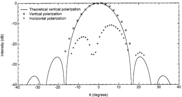
7-7 Gyrotron output at z = 5.08 cm, (a) y = 0; (b) x = 0; the solid line

represents the theoretical values, the x's the vertical polarization, and

the +'s the horizontal polarization . . . . 223

7-8 Sum of horizontal and vertical polariations at z = 5.08 cm of (a)

gy-rotron output, (b) theoretical TEO,1 waveguide mode, (c) snake output,

and (d) theoretical TE1,1 waveguide mode in a normalized dB contour

p lot . . . . 224

7-9 (a) Horizontal and (b) vertical polarizations of the snake output at

z = 5.08 cm; (c) horizontal and (d) vertical polarizations of TE1,1

theoretical intensity; normalized dB contour plot . . . . 225

7-10 Snake output at z = 5.08 cm, (a) y = 0; (b) x = 0; the solid line

represents the theoretical values, the x's the vertical polarization, and

the +'s the horizontal polarization . . . . 226

7-11 Statistical analysis of the mode converter radiation pattern assuming

two modes present in the output, the TE1,1 and TEO,1, and phase

difference. Confidence levels are indicated by solid lines. . . . . 228

7-12 Coordinate system for calculating the radiation from a circular hollow pip e [15]. . . . . 230 7-13 Setup of the apparatus for the ID radiation scans. . . . . 230

7-14 Far-field radiation scan of the output of the new snake at 41 cm using the BWO as the source. The vertical polarization is represented by

x 's, the horizontal polarization by +'s, and the theory is shown by the

solid line. The theoretical mode content of the snake is in the upper

right-hand corner. . . . . 232

7-15 Far-field radiation scan of the output of the new snake at 41 cm using

the 140 GHz gyrotron as the source. The vertical polarization is rep-resented by x's, the horizontal polarization by +'s, and the theory is shown by the solid line. The theoretical mode content of the snake is

in the upper right-hand corner. . . . . 233

7-16 Far-field radiation scan of the output of the old snake in the forward

configuration at 41 cm using the BWO as the source. The vertical polarization is represented by x's, the horizontal polarization by +'s, and the theory is shown by the solid line. The mode content of the

7-17 Far-field radiation scan of the output of the old snake in the reverse

configuration at 41 cm using the BWO as the source. The vertical polarization is represented by x's, the horizontal polarization by +'s, and the theory is shown by the solid line. The mode content of the theory data is in the upper right-hand corner. . . . 234

7-18 Photograph of the 140 GHz overmoded miter bend assembly in the

insertion loss test setup. The chopper is on the labjack on the left side and the receiver is located on the bottom. . . . 238

7-19 Corrugated waveguide transmission system for the 140 GHz gyrotron by Thomas Keating, Ltd. [16]. . . . 241

List of Tables

1.1 _{High frequency CW gyrotron oscillators . . . . 33}

1.2 _{High frequency DNP/EPR gyrotron oscillators . . . . 34}

3.1 _{Atomic mass units of residual gases present in the system measured}

with the RG A . _{. . . . 80}

3.2 _{Flow parameters for the Proteus sensors of the 460 GHz gyrotron [171. 85}

4.1 Gyrotron stability requirements for DNP/NMR spectrometer [18] . . 94

4.2 _{Gyrotron design parameters . . . . 95}

4.3 Specifications of the gyrotron magnet . . . . 109

4.4 _{Cavity design and fabrication dimensions . . . . 112}

4.5 _{Quasi-optical mode converter parameters . . . . 114}

5.1 _{Short pulse experimental operating parameters . . . . 123}

5.2 Minimum start current, and magnetic field and frequency for minimum

starting current of q = 1 modes from linear theory [19] using EGUN

calculated parameters of Fig. 4-9(a) and (b) vs. experiment . . . . . 129

5.3 _{CV experimental operating parameters . . . . 143}

5.4 _{Frequency dependence on operating parameters . . . . 147}

5.5 _{Measured and theoretical ohmic losses in the gyrotron cavity at 458 GHz 152}

5.6 _{Design and measured parameters from the ohmic loss measurement of}

the gyrotron cavity at 458 GHz . . . . 152

5.7 Cold cavity frequencies of the TE2,₃,q modes . . . . 159

5.8 _{Measured and theoretical losses in 2.54 cm diameter GlO epoxyglass}

hollow dielectric waveguides . . . . 162

5.9 _{Measured losses in various 2.54 cm diameter hollow dielectric}

waveg-uides at 460 G Hz . . . . 164

5.10 Beam waists of the mode converted radiation fields from Fig. 5-40 as

5.11 Stability of the second harmonic TEO,6 and fundamental TE2,3 modes

in the 460 GHz gyrotron . . . . 169

5.12 Cold test data and cold cavity simulation parameters of the TEo,2,q

and TE2,2,q cavity modes . . . . . 172

6.1 Frequency dependence on operating parameters of the 250 GHz

gy-rotron in the TEO,3,2 operating mode . . . . 182

6.2 Beam waist of the gyrotron output radiation field from the pyroelectric

camera and liquid crystal method . . . . 184

6.3 Stability of the 250 GHz operating parameters . . . . 187

6.4 Second harmonic modes observed in the 250 GHz gyrotron. . . . . 191

6.5 Frequency tuning for the observed modes between 5.8 and 9 T in the

250 GHz gyrotron. . . . . 193

6.6 Minimum start current, and magnetic field and frequency for minimum

starting current of q = 1 modes from linear theory [19] vs. experiment 194

6.7 Thermal load measurements on the 250 GHz gyrotron [20] . . . . 197

6.8 Cold test insertion loss measurement results with 248 ± 4 GHz radiometer209

6.9 250 GHz gyrotron beam measurements . . . . 212

7.1 Measured snake parameters . . . . 220

7.2 Theoretical mode content of the radiation field from a TE1,1 to TEO,1

mode conversion in the new snake. . . . . 231

7.3 Theoretical mode content of the radiation field from a TEO,1 to TE1,1

mode conversion in the new snake. . . . . 232

7.4 Inputs to the two-mode approach . . . . 237

7.5 Optimum two-mode approach snake parameters . . . . 237

7.6 Conversion efficiency of the snake in the multi-mode approach . . . . 238

7.7 140 GHz theoretical transmission line losses for transmission of the

TEO,1, TE1,1, and HE1,1 modes. . . . . 244

7.8 Losses in the 140 GHz transmission line in four configurations. . . . . 245

Chapter 1

Introduction

1.1

Terahertz

The terahertz or submillimeter band of the electromagnetic spectrum, corresponding to frequencies between 300 and 3,000 GHz, is of considerable interest for applications in spectroscopy, communications, high-resolution RADAR, and imaging [21, 22]. Po-tential applications are nevertheless frustrated by a historical dearth of sources that yield appreciable powers in this frequency regime. On the one hand, near-infrared lasers are capable of delivering moderate peak power at very high frequencies, but they do not yet scale to intermediate frequencies; on the other hand, conventional vacuum electron devices such as the klystron and traveling wave tube (TWT) operate at very high output powers in the tens of gigahertz, but the physical dimensions of their interaction structures (i.e. the region of interaction with the electron beam) necessarily scale with the wavelength. The resulting increase in power density with increasing frequency limits the reliability and utility of these devices above 140 GHz.

1.1.1

State-of-the-art

Figure 1-1 is a chart of source technology capable of generating high average power at submillimeter wavelengths. Unlike charts detailing the theoretical device capa-bilities, this chart is composed from data of actual continuous wave devices. The high average power devices fall into two broad categories, vacuum electron devices and lasers. Of the conventional vacuum electron devices, the carcinotron (also known as the backward wave oscillator or BWO) has carved out a niche as a compact and commercially available source generating frequencies over the 1 THz mark. In the BWO, an electron beam, focused by a magnet, passes through a periodic metallic structure and induces an electromagnetic wave, which moves in the opposite

direc-10 3

02

~10-2__

Figure 1-1: State of the art in CW terahertz sources.

tion to the electron beam. A wide frequency tuning range is available by controlling the collector potential. Unfortunately its output power at high frequencies is limited to between milliwatts and tens of milliwatts since its interaction structure is on the order of a wavelength. The far infrared (FIR) laser also seems to span the terahertz band, however has a key drawback; in a FIR laser, the frequency depends on gas type and therefore not all frequencies can be successfully generated. The quantum cascade laser (QCL), on the other hand, does not suffer from this drawback; its operating wavelength is determined by the layer thickness rather than material composition. In the QCL, electrons cascade down a series of identical energy steps (called "quan-tum wells") built into the material during crystal growth, emitting a photon at each step. Compared to diode lasers which emit only one photon over a similar cycle, it is potentially many times more powerful [23]. The present state-of-the-art for quan-tum cascade lasers at submillimeter wavelengths is 50 mW CW at 3.5 THz. The free electron laser is a vacuum electron device in which an electron beam traverses a periodic wiggler magnetic field and emits radiation. Since it requires an accelerator, its primary disadvantage is its extremely large size. A promising technology which may be extended throughout the regime is the gyrotron oscillator, which is capable of very high average power operation throughout millimeter wavelengths.

Region X Interaction of radiation with matter X-rays X-ray

o

0)

Ionization Visible 0VV\Me

energy

AnraedMolecular

Infrared

'v vvvibration

Microwave Molecular

VVV\

~

Figure 1-2: The interactions of the bands of the electromagnetic spectrum with mat-ter.

1.1.2

Interactions with matter

The interactions of the bands of the electromagnetic spectrum have varying effects upon the matter with which they interact, leading to many effects which can be harnessed for scientific applications. In this work we are interested in the effects of submillimeter radiation on matter, which tend to be less obvious than those of other bands of the electromagnetic spectrum.

X-rays (and the far ultraviolet) are classified as ionizing radiation since the quan-tum energies of x-ray photons are too high to be absorbed in electron transitions between states, and therefore can interact with an electron only by knocking it

com-pletely out of the atom (c.f. _{Fig. 1-2). When all of the energy is given to an electron,}

this is called "photoionization"; when partial energy is given to a photon and the remainder to a lower energy photon this is known as "Compton scattering," which results in a longer wavelength x-ray. The primary mechanism for the absorption of visible light photons (and near ultraviolet photons below the ionization energy) is

through the elevation of electrons to higher energy levels (c.f. Fig. 1-2). For the

visible wavelengths, we are familiar with this effect as the production of light which can be viewed by the naked eye.

The infrared region broadly covers a range of frequencies extending from the red, low frequency end of the visible spectrum (750 nm) to the far infrared (about 100 y

m). The quantum energy of infrared photons is in the range of energies separating

the quantum states of molecular vibrations (c.f. Fig.1-2). While infrared is absorbed

more strongly than microwaves, it is absorbed less strongly than visible light, result-ing primarily in heatresult-ing since it increases molecular vibrational activity. Infrared radiation can penetrate matter further than visible light.

The quantum energy of microwave photons is in the range of energies separating the quantum states of molecular rotation and torsion (c.f. Fig. 1-2). The interaction of microwaves with dielectric matter results in rotation of the molecules and which in turn generate heat from the molecular motion. A practical example is the cooking of food in a microwave oven. Most matter is transparent to microwaves, a feature which allows them to propagate over long distances and be useful for communications and radar. Another interaction of matter with microwaves involving a homogeneous magnetic field is described later in the section on nuclear magnetic resonance.

The submillimeter band includes frequencies ranging from 300 GHz to 3 THz, and is often (though not always) synonymous with "terahertz." Submillimeter pho-tons also interact with molecular rotations. While the rotational interactions with matter begin with the microwave frequencies, their strengths grow as the cube of the frequency until they reach a maximum between several hundred gigahertz and a few terahertz before dropping exponentially [21]. The molecular rotations of the submillimeter band cause complex attenuation with the Earth's atmosphere which compromise applications requiring atmospheric propagation. However the same ro-tational interactions provide strong absorptions and emissions crucial for molecular science. Another interaction of matter with terahertz involving a homoegeneous mag-netic field is described later in the section on dynamic nuclear polarization.

1.2

Cyclotron Resonance Masers

Gyrotrons, also known as cyclotron resonance masers, are robust devices. Unlike so-called "slow-wave" microwave devices, "fast-wave" devices such as gyrotron oscillators and amplifiers rely on a resonance between the modes of an interaction structure (such as the transverse electric modes of a cylindrical cavity) and the electron beam in a magnetic field. The resonator can be overmoded and, as such, can have physical dimensions which are much larger than the operating wavelength. This permits high peak and average power operation even at elevated frequencies without risk of damage to the interaction structure [241. Indeed, gyrotrons routinely achieve megawatt power levels at frequencies between 100 and 170 GHz, where plasma heating for fusion is the driving application [25]. The highest frequency achieved by a gyrotron oscillator

to date is 889 GHz at Fukui University in Japan [26]. More recent applications in spectroscopy, such as high field dynamic nuclear polarization (DNP) [27] and electron paramagnetic resonance (EPR) require lower peak power, but high average power continuous duty (7-10 days CW) operation and high stability of the frequency and output power.

1.2.1

Harmonic considerations

Superconducting magnet technology is one limiting factor in high frequency gyrotron design. At fields up to 10 T, magnets which have wide room temperature bores gener-ally employ the NbTi superconducting technology; from 10 T to 22 T (corresponding to a range of fundamental electron cyclotron frequency from 280 to 616 GHz), it is

necessary to use the Nb3Sn conductor which considerably elevates the cost of the

superconducting magnet. Resistive DC Bitter magnets, consisting of copper "Bitter" plates conceived by Francis Bitter, are currently available up to 33 T and have been used in gyrotron experiments up to 14 T [28], while hybrid magnets, combining Bitter and superconducting technology up to 45 T, though both magnet types are mainly experimental devices. Pulsed magnets can generate fields even higher, and up to 30 T have been generated synchronously with pulsed gyrotron operation [29]. This limita-tion can be alleviated by operating the gyrotron at a harmonic of electron cyclotron resonance, for which the nth harmonic will deliver n times the fundamental frequency for a given magnetic field. However, the harmonic interaction is inherently less effi-cient than the fundamental interaction due to elevated ohmic losses. It also suffers from the additional complication of mode competition and requires much higher beam currents in order to initiate oscillation. To a large extent, these difficulties can be obviated through appropriate design.

Indeed, while there has been much development of the gyrotron oscillator for fusion applications, its high frequency operation has not been similarly explored and promises to open new areas of growth. To alleviate the dense mode competition of the higher harmonic modes with the fundamental, novel cavity designs can be utilized in the place of conventional open cylindrical tapered resonators. One such mode-selective cavity is a photonic band gap (PBG) interaction structure, consisting of an array of metal rods parallel to the electron beam, where one or more rods have been removed from the center of the array to allow passage of the beam [30]. A high order transverse electric (TE) mode can exist in the "defect" if its resonant frequency lies in the band gap of the PBG structure, where the band gap can be adjusted through the geometry of the rods such that the resonant frequencies of the other modes lie in the passband of the lattice and leak out. Another novel cavity design

uses an iris, a small reduction in radius extending below cutoff, to enhance the second harmonic mode (and subsequently lower its start oscillation current) by increasing its

Q

Q

the harmonic start current. The high ohmic losses inherent in a high power, high frequency gyrotron can severely compromise the structural integrity of the interaction structure. A cryogenically cooled cavity could be employed to alleviate the thermal load. In accelerator cavities, it has been shown that copper losses can be reduced by

factors of between three and five at cryogenic temperatures [32].

1.2.2

History

The development of the gyrotron would not have been possible without the accu-mulated knowledge generated by the occurrence of numerous historical, theoretical, scientific, engineering, and physical events. To assign a concrete starting point, one can argue that the ball was set in motion in 1864 with the existence of electromagnetic waves predicted by James Clerk Maxwell. The existence of electromagnetic waves re-mained theoretical until 1888 when Heinrich Hertz experimentally demonstrated their existence by building an apparatus to produce radio waves. Subsequent technical ad-vances include the invention of a three-electrode vacuum tube (called the "triode")

by Lee de Forest in 1906. This was followed by the invention of the magnetron in 1921 by the American physicist Albert Wallace Hull, of the klystron in 1937 by the

American brothers Russell and Sigurd Varian, and of the traveling wave tube in 1943

by R. Kompfner. In 1958 and 1959, theoretical investigations on the generation of

microwaves through the electron cyclotron resonance maser interaction were carried out simultaneously by R. Twiss [33], J. Schneider [34], and A. Gaponov [35]. Finally, the earliest version of the gyrotron was developed in Russian circa 1965.

1.2.3

Operating Principles

The gyrotron, as with all microwave sources, is based on the conversion of electron beam energy into microwave radiation using a resonant structure. In many cases, an annular electron beam is produced by a magnetron injection gun and travels through a resonant cavity, located at the center of the superconducting magnet. The magnetic field causes the electrons to gyrate and thus emit radiation. If the magnetic field and cavity are tuned to match the beam parameters, the rotational energy of the electron beam will couple into a resonant cavity transverse electric mode. Figure 1-3 shows a typical cylindrical tapered gyrotron oscillator cavity of length L and radius rcavity