HAL Id: hal-03117795
https://hal-cnrs.archives-ouvertes.fr/hal-03117795
Submitted on 21 Jan 2021
HAL is a multi-disciplinary open access
archive for the deposit and dissemination of
sci-entific research documents, whether they are
pub-lished or not. The documents may come from
teaching and research institutions in France or
abroad, or from public or private research centers.
L’archive ouverte pluridisciplinaire HAL, est
destinée au dépôt et à la diffusion de documents
scientifiques de niveau recherche, publiés ou non,
émanant des établissements d’enseignement et de
recherche français ou étrangers, des laboratoires
publics ou privés.
Benjamin Marchetti, Laurence Bergougnoux, Elisabeth Guazzelli
To cite this version:
Benjamin Marchetti, Laurence Bergougnoux, Elisabeth Guazzelli.
Falling clouds of particles
in vortical flows.
Journal of Fluid Mechanics, Cambridge University Press (CUP), 2020, 908,
�10.1017/jfm.2020.883�. �hal-03117795�
Falling clouds of particles in vortical flows
Benjamin Marchetti
1, Laurence Bergougnoux
1& Elisabeth Guazzelli
21
Aix-Marseille Universit´e, CNRS, IUSTI, Marseille, France
2
Universit´e de Paris, CNRS, Mati`ere et Syst`emes Complexes (MSC) UMR 7057, Paris, France
(Received xx; revised xx; accepted xx)
The coupling between particle-particle and particle-fluid interactions is examined by studying the sedimentation of clouds of spheres in a model cellular flow at a small but finite Reynolds number. The model flow consists of counter-rotating vortices and is aimed at capturing key features of the vortical effects on particles. The dynamics of clouds settling in this vortical flow is investigated through a comparison between experiments and point-particle simulations.
Key words:
1. Introduction
In many natural phenomena or industrial applications, heavy particles are transported in complex flows. The flow structures may happen to promote the stirring and dispersion of the particles. A representative example in geophysics is the cloud or plume of ash particles coming from a pyroclastic volcanic eruption that is thrown into the atmosphere and which can spread over extremely large distance depending on wind speed and direction. But the opposite can also take place and the flow configuration may contribute to the focussing and accumulation of particles within specific regions of the flow. A typical example in the natural environment is the observed patchiness of plankton concentration caused by wind-induced Langmuir cells occurring at the surface of lakes and oceans. The objective of this paper is to explore how a collection (i.e. a cloud) of heavy particles evolves under gravity in a complex flow. The key question is whether the cloud maintains a cohesive entity or disintegrates and spreads. Most of the flow structures occurring in the environmental examples mentioned above contain coherent whirls. The present work considers a simple vortical flow, specifically a cellular flow consisting of counter-rotating vortices, and addresses the interaction of these controlled vortices with the settling cloud. The focus here is on flow regimes where inertia is small but can become finite.
A significant body of studies has been dedicated to the dynamics of settling clouds in quiescent fluids (see e.g. Noh & Fernando 1993; Nitsche & Batchelor 1997; Machu et al. 2001; Bosse et al. 2005; Metzger et al. 2007; Subramanian & Koch 2008; Pignatel et al. 2011). Different regimes have been identified depending on the magnitude of the particle and cloud Reynolds numbers (Subramanian & Koch 2008). We define the particle Reynolds number as Rea = ρfUSa/µ, where US = 2(ρp−ρf)a2g/9µ is the Stokes velocity
of an individual particle of radius a and density ρp settling in a fluid of viscosity µ
and density ρf under the gravity acceleration g, and the cloud Reynolds number as
Rec = ρfUcRc/µ, where Uc ≈ N0US6a/5Rc is the Stokes velocity of a spherical cloud of
and Rec 1, the settling of the cloud lies in the Stokes regime. While falling under
gravity, the cloud is seen to undergo an internal toroidal circulation similar to what is found for a spherical drop of heavy fluid settling in an otherwise lighter fluid (Hadamard
1911; Rybczy´nski 1911). However, this cloud becomes unstable even in the complete
absence of inertia and without the need to perturb its initial shape. It first remains roughly spherical with a leakage of particles in a vertical tail and then evolves into a torus which breaks up into two droplets in a repeating cascade. When inertia is finite, two macro- and a micro-scale inertial regimes are subsequently observed. When inertia is increased, the falling cloud transitions first to a regime dominated by macro-scale inertia
when the cloud Reynolds number becomes of order one, i.e. Rec ∼ 1. The subsequent
transition toward the micro-scale inertial regime occurs when the individual particle wakes are interacting within the cloud boundaries, i.e. when the inertial length is of the order of the cloud size, e.g. ` = a/Rea∼ Rc. In both inertial regimes, the cloud deforms
into a flat torus that eventually destabilises and breaks up into a number of secondary droplets but particle leakage is much weaker if not null. While this evolution resembles that observed in the Stokes regime, the physical mechanisms involved are qualitatively different. Whereas the inertial cloud evolution is strongly determined by the importance of wake-mediated interactions, the key feature of the Stokes cloud is the chaotic motion of the particles which leads to escapes from the cloud internal circulation and to particle leakage. Simulations using point-particle approaches, which contain the minimal physics of the multibody particle interactions, capture these dynamics (Nitsche & Batchelor 1997; Bosse et al. 2005; Metzger et al. 2007; Pignatel et al. 2011).
If the particle cloud settles now in a flowing fluid instead of a quiescent fluid, there are interactions not only between the particles but also between the particles and the local spatial structures of the flow (e.g. large vortices). The literature on sedimentation of heavy particles in non-uniform flows, and specially in random or turbulent flows, has shown the important effect of these vortical structures on the local particle transport and concentration, in particular through a phenomenon known as preferential sweeping where particle paths accumulate at the periphery of the vortical structures (see e.g. Wang & Maxey 1993; Aliseda et al. 2002; Toschi & Bodenschatz 2009; Balachandar & Eaton 2010). Preferential sweeping is generally considered responsible for the turbulence to increase the settling velocity of inertial particles but other mechanisms, such as vortex trapping and loitering or nonlinear drag effects, have also been proposed for, on the contrary, reducing the settling velocity (see e.g. Nielsen 1993; Mei 1994; Good et al. 2014; Akutina et al. 2020). These features can be also seen using a model cellular flow of counter-rotating vortices. At low particle Reynolds number, individual particles settle at their Stokes velocity simply augmented by the local fluid velocity (Stommel 1949). Their trajectories can be classified according to the magnitude of the ratio of the Stokes velocity, US, to the vortex velocity, U0, i.e. the parameter W = US/U0. When W > 1,
the trajectories are essentially straight vertical line as the particles settle through the
vortex array without being mostly influenced by it. For W ≈ 1, the particles are affected
by the local flow and the trajectories can exhibit zigzagging motions depending on their position of release within the vortex array. For smaller values of W , the particles can be suspended in the flow. When inertia is increased, the dynamics of single individual particles has been described by the Boussinesq-Basset-Oseen equation (Gatignol 1983; Maxey & Riley 1983). The major influence of inertia on the motion is that the particles cannot be resuspended in the flow and are seen to settle out even when they are trapped momentarily into a vortex (Maxey 1987). This effect has been observed in experiments using a cellular flow field created by electroconvection (Bergougnoux et al. 2014). The experiments show that, for small values of the Stokes number, St (defined as the ratio
of the particle response time to the characteristic time of the flow), added mass and history forces are inconsequential and that the dominant forces are buoyancy and drag provided that the Stokes drag is replaced by a nonlinear drag depending of the particle Reynolds number. Collective effects between the particles may also affect this settling but they do not have been thoroughly addressed. The role of particle clusters and their association with settling velocity enhancement has been pointed in Stokes sedimenting flows (Guazzelli & Hinch 2011) but also more recently in the turbulent regime (Huck et al. 2018).
The objective of the present work is to tackle the interplay between the multibody particle interactions and the interaction between the particles and the spatial structures of the flow. This coupling is examined for a cloud settling in a cellular flow field which is a simple model flow capturing key features of vortical effects on the particles. In
the experiments described in§ 2, electroconvection is used to generate a two-dimensional
array of controlled vortices and clouds of particles are released and tracked in this vortical
flow. The observed cloud dynamics is compared in§ 4 against point-particle simulations
described in§ 3. Conclusion are drawn in § 5.
2. Experiments
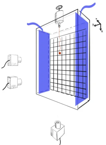
The experimental apparatus consists of a cell made of Plexiglas (of 50 cm height, 38 cm width, and 4 cm depth) filled with an aqueous mixture of citric acid (a certain amount of UCON R oil can be added to increase the fluid viscosity), as depicted in figure 1. The
vortical flow is created by electromagnetic convection. The magnetic field is produced by
a checkerboard of permanent square magnets (2× 2 cm2) placed against the back wall of
the cell. An electrical current is generated between two carbon electrodes placed on the opposite small sides of the cell. The coupling between the magnetic field and the uniform electric current gives rise to an electromagnetic force in the fluid. This induces a flow of counter-rotating vortices having the same size as the magnets and an intensity controlled by the magnetic field of the permanent magnets, the intensity of the electric current, and the viscosity of the fluid. Further details can be found in Bergougnoux et al. (2014) and Lopez & Guazzelli (2017).
The flow generated by electroconvection is characterised by particle image velocimetry (PIV). For this purpose, the fluid is seeded by tracer particles (hollow spheres with
diameter ≈ 15 µm and density ≈ 1.4 g.cm−3 from Dantec Measurement Technology)
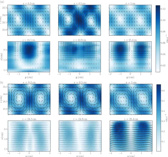
and is illuminated by a green laser sheet which can be positioned in the vertical or horizontal planes. A camera is focused on the illuminated particles which scatter the light and records two images separated in time by typically 1/7 to 1/15 s. These images are processed to find the velocity-vector map of the flow field using the Matlab PIV software DPIVsoft (Meunier & Leweke 2003). The resulting three-dimensional flow field possesses a quasi two-dimensional periodic structure of counter-rotating vortices of size L = 2 cm (i.e. with a spatial wavenumber k = 2π/2L) in the vertical plane having an
intensity which reaches a maximum at x ≈ 5 mm away from the back wall and then
decays rapidly. This cellular flow is close to a Taylor-Green cellular flow when the flow Reynolds number is small, i.e. for Rek = U0k−1/(µ/ρf) < 1, see figure 2 (a). For larger
values of Rek, the spatial structure can be slightly distorted and three-dimensional, see
figure 2 (b). It eventually becomes unstable for Rek> 15.
Clouds are prepared by mixing a weighted amount of spherical particles with the same fluid as that filling the cell, see tables 1 and 2 describing the characteristics of the different fluids and particles which have been used. This suspension mixture is dropped
Figure 1. Experimental apparatus. The transparent cell is filled with an aqueous mixture of citric acid (UCON R
oil can be added to increase the viscosity). The magnetic field is generated by a checkerboard of magnets placed behind the back wall of the cell. The electric current is created by two electrodes placed on the opposite small sides of the cell. The flow generated by this set-up is a periodic flow of counter-rotating vortices that is depicted in figure 2. Clouds are dropped from the top of the cell using a custom made syringe and settle through the cellular flow. Their trajectories are imaged by a set of synchronised cameras located below and in front of the cell.
Batch a (µm) ρp(g cm−3)
A 70 ± 6 1.049 ± 0.003
B 115 ± 14 1.049 ± 0.003
C 175 ± 20 1.189 ± 0.001
Table 1. Particle characteristics: mean sphere radius a (the error bar corresponds to the
standard deviation) and density ρp. Batches A and B are made of polystyrene particles while
batch C consists of polymethyl methacrylate (PMMA) particles.
the maximum plateau location of the vortex intensity. The injected cloud settles first in the quiescent fluid and then, as electroconvection is activated, through the vortical flows. A set of synchronised cameras located below and in front of the cell tracks the cloud both in the vertical and horizontal plane. Standard digital imaging treatments (first the ‘threshold’ function and then the ‘particle-analyse’ function of ImageJ) yield
23.5 24.0 24.5 25.0 z (cm) (a) x = 0.2 cm x = 0.5 cm x = 1 cm −2 −1 0 1 2 y (cm) 0.5 1.0 1.5 x (cm) z = 24.5 cm −2 −1 0 1 2 y (cm) z = 24.9 cm −2 −1 0 1 2 y (cm) z = 25.4 cm 0.02 0.04 0.06 0.08 0.10 0.12 cm .s − 1 23.5 24.0 24.5 25.0 z (cm) x = 0.2 cm x = 0.5 cm x = 1 cm −2 −1 0 1 2 y (cm) 0.5 1.0 1.5 x (cm) z = 24.5 cm −2 −1 0 1 2 y (cm) z = 24.9 cm −2 −1 0 1 2 y (cm) z = 25.4 cm 0.1 0.2 0.3 0.4 0.5 0.6 cm .s − 1 (b)
Figure 2. Vortical flow: velocity-vector map of the flow field in the vertical plane (zy) for different horizontal positions (x) and in the horizontal plane (xy) for different vertical positions
(z) in cases (a) A1a (Rek= 0.7) and (b) C2b (Rek= 13.6).
Fluid Mixture µ (cP) ρf(g cm−3)
1 83% water + 10% UCON R oil + 7% citric acid 10.0 ± 0.1 1.042 ± 0.001
2 64% water + 36% citric acid 3.3 ± 0.2 1.173 ± 0.001
Table 2. Fluid characteristics: viscosity µ and density ρf.
the time-evolution of the position of the centre of mass of the cloud, X, Y , and Z, and of some other quantities such as its projected surface in the horizontal plane, Σ. The detection of the cloud dynamics is undertaken until the cloud begins to break, i. e. when the cloud starts to bend to break into pieces. The time-evolutions of the clouds have been examined for different combinations of particles and fluid mixtures listed in table 3
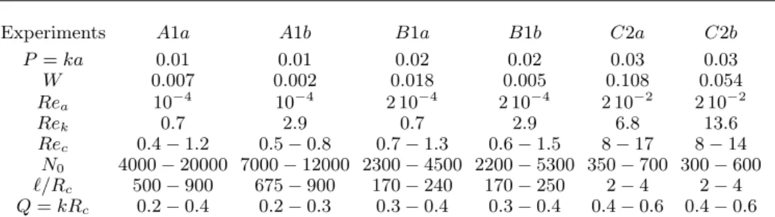
which also indicates different dimensionless parameters (P = ka, W , Rea, Rek, Rec,
N0, `/Rc, Q = kRc). Note that for each combination, two different current intensities
Experiments A1a A1b B1a B1b C2a C2b P = ka 0.01 0.01 0.02 0.02 0.03 0.03 W 0.007 0.002 0.018 0.005 0.108 0.054 Rea 10−4 10−4 2 10−4 2 10−4 2 10−2 2 10−2 Rek 0.7 2.9 0.7 2.9 6.8 13.6 Rec 0.4 − 1.2 0.5 − 0.8 0.7 − 1.3 0.6 − 1.5 8 − 17 8 − 14 N0 4000 − 20000 7000 − 12000 2300 − 4500 2200 − 5300 350 − 700 300 − 600 `/Rc 500 − 900 675 − 900 170 − 240 170 − 250 2 − 4 2 − 4 Q = kRc 0.2 − 0.4 0.2 − 0.3 0.3 − 0.4 0.3 − 0.4 0.4 − 0.6 0.4 − 0.6
Table 3. Dimensionless numbers for the different combinations of particles (labelled A, B, and C), fluids (labelled 1 and 2) and current intensities (labelled a and b) used in the experiments.
Figure 3. Typical three-dimensional trajectories of centres of mass of clouds. The colour coding (colour online) corresponds to the distance to the back wall, and the trajectories projected in the horizontal plane are shown at the bottom. The trajectories which do not possess a large x-extension are selected.
different values of vortex velocities, U0. Note also that the cloud size is always smaller
(by a factor ten) than the size of the vortices. For each experimental condition listed in table 3, typically 4-5 experimental runs have been performed but only trajectories which are not too close to the walls and do not have a large x-extension are retained. Typical three-dimensional trajectories of centres of mass of clouds are depicted in figure 3.
3. Numerical modelling
We consider N0 spherical particles initially randomly distributed in a sphere of radius
Rc(or alternatively in a prolate spheroid of same volume to mimic the initial shape of the
cloud obtained in the experiments) settling under gravity in a vortical flow field uvortex
characterised by a spatial wavenumber k and a vortex intensity U0. We adopt the simplest
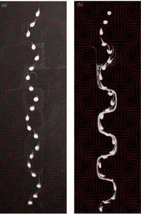
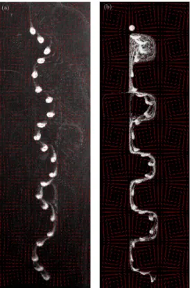
(a) (b)
Figure 4. Typical (a) experimental and (b) numerical chronophotographies of a cloud for case A1b. The time between successive photos is kept constant (2 s in the experiments and a corresponding interval in the simulation) in order to indicate the difference in velocities along the trajectory. The flow field measured by PIV is indicated by red arrows. The complete dynamics for the experimental case and for the Stokeslet simulation are shown in supplementary movie 1.
in which particles are represented by identical point forces. Within this approximation, the velocity, ˙rα
i, of a particle α located at a position rαi is its own Stokes velocity US
incremented by the local fluid velocity at riα(Stommel 1949) and the sum of the velocity disturbances (only represented by its far-field portion, i.e. the Stokeslet) coming from the other particles β located at a position rβi (see e.g. Metzger et al. 2007). Using k−1
as the length scale and U0 as the velocity scale, the dimensionless equations of motion
(with dimensionless quantities denoted with a hat) are written as ˆ˙rαi = ˆu vortex i (ˆr α i) + W δi3+ 3 4P W X β6=α " δi3 ˆ rαβ + ˆ rαβi rˆαβ3 (ˆrαβ)3 # , (3.1)
where rαβi = riα− rβi and rαβ =|rαi − riβ|. We have used the dimensionless parameters
P = ka and W = US/U0.
To test the effect of a vertical wall on the cloud dynamics, we have followed Blake (1971) and implemented a mirror image system of the point forces enabling to satisfy the no-slip condition on the wall boundary. The typical evolution with or without the wall is essentially identical as pointed by My lyk et al. (2011) for a cloud falling in a quiescent fluid. We have verified that, for a distance to the wall larger than a few cloud radii as achieved in the experiments, the effect happens to be insignificant.
Figure 5. Same as figure 4 but for case B1b. The complete dynamics for the experimental case and for the Stokeslet simulation are shown in supplementary movie 2.
number (i.e. the ratio of the particle response time, ∝ ρpa2/µ, to the flow time scale,
∝ 1/kU0, St ∝ a2ρpkU0/µ) is still small (St ≈ 2 10−3 for case C2a and ≈ 4 10−3 for
case C2b), the assumption of linearity can be maintained but instead of a Stokes drag a nonlinear drag may be used, e.g. a Schiller-Naumann drag (Bergougnoux et al. 2014). As a first estimate, the far-field Stokes interactions can also be replaced by the steady far-field Oseen interactions (i.e. the Oseenlet) in equation (3.1) to encompass the inertial wake interactions between particles (Subramanian & Koch 2008; Pignatel et al. 2011). This is however a crude approximation as assuming steady Oseen wake interactions is far from being justified (see e.g. Lovalenti & Brady 1993). The new dimensionless equation of motion then reads
ˆ˙rαi = ˆu vortex i (ˆr α i) + W δi3+ 3 4P W X β6=α ( ˆ riαβ (ˆrαβ)2 " 2ˆ` ˆ rαβ(1− ˆE)− ˆE # + ˆ E ˆ rαβδi3 ) , (3.2)
where the inertial screening length is ` = a/Rep and E = exp
h −(1 +rαβ3 r ) rαβ 2` i .
Knowing the initial positions of the N0 particles at time t = 0, the sets of equations
(3.1) or (3.2) represent a close system of 3N0coupled ordinary differential equations which
can be numerically integrated for a cellular flow uvortex inferred from interpolating the
three-dimensional PIV measurements of the flow field described in § 2. The integration
has been performed using an explicit Runge-Kutta method of order (4)5 (the ‘dopri5’ integrator of the ‘ode’ solver in Python). To optimise and run the Python code with a large number of point-particles, we use the Numba package to translate the mobility-matrix function written in Python into a fast native machine code. The numerical
(a) (b)
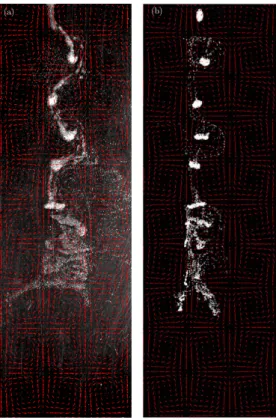
Figure 6. Same as figure 4 but for case C2b. The numerical simulation uses an Oseenlet (instead of Stokeslet) approximation. The complete dynamics for the experimental case and for the Oseenlet simulation are shown in supplementary movie 3.
trajectory of each particles of the initial spherical cloud can then be obtained and analysed. The generated images of the clouds can also be treated in a similar manner as in the experiments to give the trajectory and shape of the numerical clouds for a close comparison examination.
4. Results and comparison
In the following, we present the experimental results of the time-evolution of the cloud and compare them to the numerical predictions obtained using the point-particle
approaches introduced in§ 3. This latter numerical modelling also enables access to some
dynamical features which are not amenable in the experiments. We investigate the Stokes regime but also the effect of increasing finite inertia. Before embarking in these analyses, it is important to consider the various dimensionless parameters involved in the problem. For Stokes clouds settling in a quiescent fluid, the only relevant parameter is the initial
number of particles, N0. For Stokes clouds settling in a vortical flow of intensity U0
and size k−1, two additional dimensionless numbers come into play, the velocity ratio
W = US/U0 and the size ratio P = ka or alternatively Q = kRc. When inertia is
increased, it is important to consider additionally the cloud Reynolds number, Rec, and
the particle Reynolds number, Rea, or alternatively the dimensionless inertial length k` or
`/Rc. It is important to mention that the Stokes number, St∝ a2ρpkU0/µ (≈ 2 − 4 10−3
for the most inertial cases C2a and C2b), and size ratio, P = ka (≈ 0.01 − 0.03), of
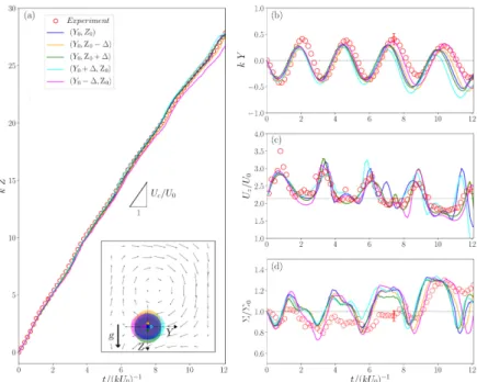
Figure 7. Typical experimental (◦) and numerical (solid lines) trajectories in the Stokes case B1a: time evolution of the (a) vertical, Z, and (b) horizontal, Y , coordinates of the cloud centre of mass, (c) its vertical velocity, Uz, and (d) the cloud projected surface in the horizontal
plane normalised by its initial value, Σ/Σ0. In graph (a), the black triangle indicates the slope
Uc = N0US6a/5Rc and the inset shows the initial positions of the cloud within experimental
accuracy ∆ (with k∆ = 7 10−2). The horizontal dotted lines correspond (i) to the initial location kY = 0 in graph (b), (ii) to the value Uc/U0in graph (c), and (iii) to the initial projected surface
Σ/Σ0= 1.
number of the cloud itself is larger, typically (Rc/a)2 larger, leading to values≈ 1 for
the most inertial cases C2a and C2b. The cloud radius is always smaller than the spatial
wavelength of the vortical structure (Q = kRc ≈ 0.2 − 0.6) because of the small
x-extension wherein the cloud can be dropped and for which the vortex intensity can be kept constant away from the back wall (see figure 2).
4.1. General evolution of the clouds
The typical evolution of a cloud settling in the vortical flow in the Stokes regime (case A1b) is shown in the chronophotography of figure 4 (a). The cloud is seen to settle along the downstream flow of the successive vortices and to display zigzagging motions due to the modulations caused by the periodic cellular flow. It does not maintain a spherical shape as it is slightly stretched in the elongational region of the flow, in particular close to the stagnation points surrounding the purely rotational regions at the centres of the vortices. A significant leakage of particles is observed at its rear and the released particles move with the vortical flow and thus can be trapped into the vortices as the ratio of their Stokes velocity to the flow velocity, W (= 0.0017), and their Reynolds number,
Rea(= 10−4), are both very small. No break-up is observed as the travel distance of
the cloud is not long enough for this phenomenon to happen. The cloud falls across 12 vortices (≈ 100 times its radius) and it would necessitate for the cloud to fall at least 500 times its radius for break-up to occur in the Stokes regime (Metzger et al. 2007). Similar qualitative evolution is found between the point-particle simulation using the Stokeslet approximation and the experiment in this regime as evidenced by comparing figure 4 (a)
0 2 4 6 8 10 0.0 0.5 1.0 1.5 0 2 4 6 8 10 0.0 0.5 1.0 1.5 2.0 2.5 0 2 4 6 8 10 t/(kU0)−1 0.0 0.5 1.0 1.5 2.0 2.5 3.0 0 2 4 6 8 10 t/(kU0)−1 0 2 4 6 8 10 12 14 k Z Experiment (a) (Y0, Z0) (Y0, Z0− ∆) (Y0, Z0+ ∆) (Y0+ ∆, Z0) (Y0− ∆, Z0) k Y Σ / Σ0 Uz /U 0 (b) (c) (d) g Y Z 1 Uc/U0
Figure 8. Same as figure 7 but for the finite-inertia case C2b. The ? symbols indicate break-up events.
and (b). However, the experiments show a mostly rounded shape of the cloud while the simulations give more like a mushroom shape. This discrepancy is observed for case A1b having a cloud with a large number of particles (see table 3) and may be due to excluded-volume effects not accounted for in the point-particle simulations. The behaviour of the cloud for case B1b is displayed in figure 5 and presents similar features as for case A1b since inertia is still very small. The cloud deformation by the flow structure is however stronger. This is even more significant when inertia becomes finite for case C2b shown in figure 6. The cloud is highly deformed and eventually widens in the upward elongational portion of the flow and breaks into multiple pieces. Point-particle simulations using an Oseenlet (instead of Stokeslet) approximation can capture this phenomenon.
4.2. Cloud trajectory
A more quantitative comparison between experiments and simulations can be obtained by examining the time evolution of the vertical, Z, and horizontal, Y , coordinates of the
cloud centre of mass, its vertical velocity, Uz, and the cloud projected surface in the
horizontal plane normalised by its initial value, Σ/Σ0.
In a typical Stokes case (B1a) depicted in figure 7, Z(t) is approximatively a straight line while Y (t) exhibits oscillations due to the modulation induced by the vortical flow. The mean settling velocity of the cloud is similar to that observed when falling in a quiescent fluid, Uc ≈ N0US6a/5Rc, as shown in figure 7 (a). Its vertical velocity Uz(t)
and the normalised projected surface Σ(t)/Σ0experience periodic oscillations. The cloud
slows down (accelerates, respectively) while simultaneously expanding (shrinking, respec-tively) when it falls through the successive upward (downward, respecrespec-tively) elongational portions of the flow. Numerical simulations using the Stokeslet approximation are also presented in figure 7 for N0= 2500 corresponding to the experimental value. The different
curves correspond to simulations having different initial positions for the cloud centre of mass which are chosen within the experimental accuracy of the cloud initial location.
Figure 9. Snapshots of the settling numerical cloud for cases (a) B1a (N0 = 2500) and (b)
C2b (N0= 500). The original flow field measured by PIV is indicated by black arrows while the
perturbed flow field is represented by blue streamlines. The corresponding movies are available in the supplementary material (movie 4 for the Stokeslet simulation and movie 5 for the Oseenlet simulation).
More precisely, the initial position is shifted along the vertical or horizontal directions by the experimental error ∆ on the initial location, as indicated in the legend of graph (a). The set of obtained curves encloses the experimental data, and in particular, the amplitude and phase of the oscillations are captured in graphs (b), (c), and (d) of figure 7. Dispersion and phase shift between the different curves are seen to increase slightly with time because of the sensitivity to the local velocity field, in particular at the stagnation saddle points, as observed previously for individual particles (Bergougnoux et al. 2014). In the finite-inertia case (C2b), the trajectories can be followed only over a distance of ≈ 4 − 5 vortices since break-ups (indicated by the ? symbols) quickly occur, as shown in figure 8 for a typical example. The vertical position Z(t) again follows approximately a straight trajectory with a slope≈ Uc while the horizontal position Y (t) presents
oscilla-tions. The normalised projected surface Σ(t)/Σ0experiences similar periodic oscillations.
Conversely, the vertical velocity Uz(t) shows oscillations but with a doubled period
compared to those of Y (t). This is a sign of the successive slowdowns and accelerations during the fall of the cloud through a vortical structure. This period doubling was not distinctly seen in the Stokes case of figure 7 (c). Numerical simulations using the Oseenlet
approximation (with N0 = 500 to match the experimental condition) capture these
behaviours. Some discrepancy is observed for Σ(t)/Σ0. It may be due to experimental
error in the determination of Σ coming from difficulties to discriminate between the particles within or without the cloud (this is enhanced after some settling distance when the tail behind the cloud due to particle leakage becomes important).
Comparison between behaviours in the viscous and inertial cases is shown in figure 9 where snapshots of the numerical clouds are shown during settling for cases (a) B1a
(N0= 2500) and (b) C2b (N0= 500). The perturbed streamlines are represented together
with the original PIV flow fields. The vortices are pushed apart when the cloud is falling in a downward portion of the flow between the two vortices while they are pulled closer when the cloud sweeps around the vortical structure when there is an upward flow between the two vortices. The oscillations between the expansions and contractions of the cloud when settling in the successive upward and downward, respectively, portions of the flow are clearly seen. This phenomenon seems to be enhanced in the Oseenlet simulation wherein the upward elongational flow favours the cloud expansion.
4.3. Particle leakage from the cloud
Since the evaluation of particle leakage from the cloud is difficult to achieve in the experiments, we have chosen to rely on numerical simulations. To identify the particles lo-cated inside the cloud, a connected-component-labeling algorithm has been used to detect connected regions in the binary digital images and to identify blob regions, in particular the cloud entity. First, we construct a boolean matrix containing the coordinates of the particles with an element resolution corresponding to the interparticle distance. Second, we use the connected-component-labeling algorithm (function measure.label in Python skimage library) which identifies blobs of adjacent elements and labels the different blobs. Then, the cloud entity is determined as the blob having the highest coordinates along z; the other blobs of particles are considered as leaking from the cloud. Figure 10 shows the
percentage (N0− N)/N0of particles that have leaked away from the cloud as a function
of time. The data correspond to averages over 10 numerical simulations having different initial particle distributions using the Stokelet (cases A1a and B1b) and the Oseenlet (case C2b) models.
Figures 10 (a) and (b) compare leakage obtained when the cloud is settling in (a) quiescent fluids and (b) vortical flows. They clearly evidence that the leakage is intensified by the vortical flows. Strikingly, while leakage is small when Oseenlet clouds settle in
0.00 0.01 0.02 0.03 0.04 0.05 0.06 (N 0 − N )/ N0 − N0 B1b− N0= 2500 C2b− N0= 500 Break-up 0.0 0.1 0.2 0.3 0.4 0.5 0.6 0.0 0.1 0.2 0.3 0.4 0.5 0.6 0.7 (N 0 − N )/ N0 (c) B1b− N0= 1000 B1b− N0= 1500 B1b− N0= 2000 B1b− N0= 2500 0.0 0.1 0.2 0.3 0.4 0.5 0.6 0.7 (d) C2b− N0= 500 C2b− N0= 1000 C2b− N0= 1500 C2b− N0= 2000 Break-up 0 10 20 30 40 50 60 tUc/Rc 0.0 0.1 0.2 0.3 0.4 0.5 0.6 0.7 (N 0 − N )/ N0 (e) Rek= 0.7 Rek= 2.9 0 10 20 30 40 50 60 tUc/Rc 0.0 0.1 0.2 0.3 0.4 0.5 0.6 0.7 (f ) Rek= 6.8 Rek= 13.6 Break-up 100 10tU1c/Rc 102 100 101 102 (N 0 − N )/ N 1/ 3 0 2/3 100 101 102 tUc/Rc 100 101 102 (N 0 − N )/ N 1/ 3 0 1
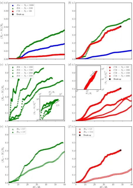
Figure 10. Percentage (N0− N )/N0 of particles that have leaked away from the cloud as a
function of dimensionless time tUc/Rc: in (a) quiescent fluids and (b) vortical flows for cases
A1a, B1b, and C2b; in vortical flows for different N0 for cases (c) B1b and (d) C2b; in vortical
flows for two different Rek for cases (e) B1b and (f) C2b. The insets of graph (c) and (d) show
the same leakage N0− N but normalised by N01/3instead of N0.
quiescent fluids (Pignatel et al. 2011), it is amplified by a factor of ≈ 90 when these
clouds fall in vortical flows. Figures 10 (c) and (d) show that the rate of leakage decreases as the initial number N0is increased in both the (c) viscous (B1b) and (d) inertial (C2b)
cases for cloud settling in vortical flows. Normalising the leakage N0−N by N 1/3
0 instead
of N0produces a collapse of the data onto a master curve at long time and for sufficiently
large N0, as previously seen for clouds falling in quiescent fluids (Metzger et al. 2007). For
tUc/Rc> 10, (N0− N)/N 1/3
Experiments Oseenlet Simulation Oseenlet Simulation
N0= 300 − 600 N0= 500 N0= 1000
in quiescent fluid 115 ± 28 63 ± 5 62 ± 3
C2a 29 ± 6 16 ± 3 –
C2b 26 ± 5 21 ± 3 –
Table 4. Dimensionless break-up times, tbUc/Rc, in the quiescent and vortical cases (C2a and
C2b). The error bars correspond to the standard deviations between the different experimental or numerical runs.
obtained for Stokes clouds settling in quiescent fluids (Metzger et al. 2007). This contrasts
with the scaling as tUc/Rc which seems to be obtained in the inertial case. This again
evidences the strong increase of leakage by the vortical flow when inertia becomes finite. Figures 10 (e) and (f) show that increasing the Reynolds number of the flow intensifies the leakage, in both viscous (for N0= 2500) and inertial (for N0= 500) cases. It is worth
noticing that the percentage of leakage presents oscillations induced by the modulation of the cellular flows in graphs (b), (c), (d) (e), and (f). This is likely to be linked to the modulation of the size of the cloud when falling through the vortical structure as shown in figure 9. The cloud seems to loose particles when it is shrinking, i.e. when falling in a downward elongational portion of the flow, see figure 9(b) at t/(kU0)−1= 3.8.
4.4. Break-up of the cloud
As mentioned previously in § 4.1, break-up events have been only observed in the
finite-inertia case and thus are only analysed in that regime. The key quantity is the
time required to reach the break-up, tb, which characterises the lifetime of the cloud.
This time can be inferred as the time for which the cloud starts to bend to break into pieces. Table 4 gives the dimensionless break-up time, tbUc/Rc, for clouds of particles C
settling in fluid 2 both in the quiescent case and in the vortical cases (C2a and C2b). The experimental data correspond to averages over typically 10 runs and the error bars to the standard deviations over the different runs. Clearly, break-up times are shorter when clouds are settling into vortical flows. Numerical simulations using the Oseenlet
approximation have been performed for similar inertial length, `/Rc≈ 2 − 3, and initial
size of the cloud, Q = kRc ≈ 0.5, and for N0 = 500 (and also 1000 in the quiescent
case). The numerical data correspond to averages over 5-10 runs having differing initial distributions but also having different initial positions for the centre of mass as done in
figures 7 and 8 of § 4.2. The trend is similar to that observed in experiments although
the numerical values are somehow smaller than those found experimentally. This latter discrepancy may be due to the fact that the present numerical model is not accounting for unsteady or excluded-volume effects.
A physical picture of the mechanism leading to break-up can be obtained from a visualisation of the flow field in the cloud reference frame for a typical Oseenlet simulation in case C2b, see figure 11. As mentioned before in discussing figure 9, the cloud successively expands and contracts when falling in the consecutive upward and downward, respectively, elongational portions of the flow. When inertia is finite, the oscillation between the expansion and contraction phases is no longer reversible and the cloud expansion becomes stronger. When the cloud reaches an upward elongational region of the flow wherein there is a slow-down of the velocity, break-up then happens as the
Figure 11. Flow field computed at successive times in the vertical plane in the cloud reference frame for a typical Oseenlet simulation in case C2b. High (low) velocity is indicated in white (dark). The corresponding movie 6 is available in the supplementary material.
8.3, and 8.8. The remaining pieces of the cloud spread in the flow structures and can
undergo the same break-up process, see the graph at t/(kU0)−1= 10.1.
5. Concluding remarks
We have performed experimental investigations as well as numerical simulations to examine the dynamics of clouds of particles settling in model cellular flows consisting of counter-rotating vortices where inertia is small but can be increased to become finite.
Figure 12. Snapshots of numerical clouds (using the Oseenlet approximation) corresponding
to case C2a (P = 0.03, W = 0.108, `/Rc= 2) settling in Taylor-Green vortices at five different
times ˆt = t/(kU0)−1 = 0, 8, 16, 24, 32 (each time ˆt corresponds to a different colour) with (a)
Q = 0.5 and N0= 500, (c) Q = 2 and N0 = 500, and (e) Q = 2 and N0= 2000. Conditions in
(b), (d), (f) are the same as in (a), (c), (e), respectively, but hydrodynamic interactions between particles have been switched off. The corresponding movie 7 is available in the supplementary material.
The clouds tend to settle along the downstream flow regions of the vortical structures and to present zigzagging motions. They do not maintain their initial spherical shape as they successively expand or shrink when settling through the successive upward or downward elongational portions of the flow. Increasing inertia enhances the cloud deformation. A significant leakage of particles is observed at the rear of the clouds. It is greatly amplified by the vortical flows by comparison with clouds settling in quiescent fluids. It is also intensified when inertia is increased and becomes finite. The vortical structures also induce a faster break-up of the clouds into multiple shatters in the finite inertia case. Point-particle simulations, which contain the minimal physics to describe the coupling between particle-particle and particle-flow interactions, capture well the cloud dynamics. A key feature that is highlighted in the present work is the importance of the collective effects between the particles in maintaining the cloud as a single entity before break-up occurs owing to stretching in the vortical flow. This can be further investigated in figure 12 by going beyond the experimental constraint of having an initial cloud smaller than the vortex size, i. e. by investigating a cloud with Q > 1. When the size of the initial
cloud is larger than that of the vortices, the cloud can break into pieces which can be further stretched by the elongational regions of the flow. This is shown by comparing
figures 12 (a) and (c) having the same N0 = 500 but with Q = 0.5 and 2, respectively.
Increasing the number of particles increases the cohesion of the cloud which is eventually stretched into elongated pieces by the vortical structure as seen in figure 12 (e) having
the same Q = 2 as figure 12 (c) but a different N0 = 2000. The cloud in figure 12 (e)
falls at a faster pace than that in figure 12 (c) since the cloud velocity is Uc∼ N0. As a
comparison, we also show simulations in figures 12 (b), (d), (f) corresponding to the same initial cloud as in figures 12 (a), (c) and (e), respectively, but wherein the hydrodynamic interactions have been switched off. The difference between the simulations with and without collective effects (i. e. with and without two-way coupling) is striking. Without hydrodynamic interactions, the individual particles settle much slowly as they sweep around the vortices since W = 0.108 < 1 and a significant amount of them remains trapped inside the vortex circulations since the Reynolds number based on the individual particle size is Rea 1.
Another interesting output of the present study is the identification of a mechanism of expansion and contraction of the cloud leading to a final disintegration into multiple stretched pieces induced by the elongational portions of the vortical flow when inertia is increased (see figures 11 and 12). This last effect may be related to particle segregation in turbulent flow which has been seen to evolve into a network of filamentous shapes similar to caustic patterns (see e. g. Reeks 2014). The generation of such inhomogeneities in the context of particles sinking in oceanic flows has been attributed to stretching mechanisms
due to the flow (Dr´otos et al. 2019). More work is certainly needed to assess whether
stretching by the elongational part of the flow structure is a generic and robust process that is seen in more complex flow than the model vortical flow studied in the present work.
Acknowledgments
This article has been written under the auspices of the ANR project “Collective Dynamics of Settling Particles In Turbulence” (ANR-12-BS09-0017-01), the ‘Laboratoire
d’Excellence M´ecanique et Complexit´e’ (ANR-11-LABX-0092), the Excellence Initiative
of Aix-Marseille University - A∗MIDEX (ANR-11-IDEX-0001-02) funded by the French
Government “Investissements d’Avenir programme”, and COST Action MP1305 ‘Flow-ing Matter’. We thank D. Lopez, J. Massoni, and J. Vicente for help in data acquisition and processing and E. Climent and A. Soldati for discussions and comments.
Declaration of Interests
The authors report no conflict of interest.
REFERENCES
Akutina, Y, Revil-Baudard, T, Chauchat, J & Eiff, O 2020 Experimental evidence of settling retardation in a turbulence column. Phys. Rev. Fluids 5, 014303.
Aliseda, A, Cartellier, A, Hainaux, F & Lasheras, JC 2002 Effect of preferential concentration on the settling velocity of heavy particles in homogeneous isotropic turbulence. J. Fluid Mech. 468, 77–105.
Balachandar, S & Eaton, John K 2010 Turbulent dispersed multiphase flow. Annu. Rev. Fluid Mech. 42, 111–133.
Bergougnoux, L, Bouchet, G, Lopez, D & Guazzelli, ´E 2014 The motion of solid spherical particles falling in a cellular flow field at low Stokes number. Phys. Fluids 26, 093302–15. Blake, J R 1971 A note on the image system for a stokeslet in a no-slip boundary. Proc.
Cambridge Philos. Soc. 70, 303–9.
Bosse, T, Kleiser, L, H¨artel, C & Meiburg, E 2005 Numerical simulation of finite Reynolds
number suspension drops settling under gravity. Phys. Fluids 17, 037101–17.
Dr´otos, G, Monroy, P, Hern´andez-Garc´ıa, E & L´opez, C 2019 Inhomogeneities and
caustics in the sedimentation of noninertial particles in incompressible flows. Chaos 29, 013115–26.
Gatignol, R 1983 The Faxen formulae for a rigid particle in an unsteady non-uniform Stokes flow. J. M´eca. Th´eo. Appli. 2, 143–160.
Good, G H, Ireland, P J, Bewley, G P, Bodenschatz, E, Collins, L R & Warhaft, Z 2014 Settling regimes of inertial particles in isotropic turbulence. J. Fluid Mech. 759, R3. Guazzelli, E & Hinch, J 2011 Fluctuations and instability in sedimentation. Annu. Rev. Fluid
Mech. 43, 97–116.
Hadamard, J 1911 Mouvement permanent lent d’une sph`ere liquide et visqueuse dans un liquide
visqueux. C. R. Acad. Sci. (Paris) 152, 1735–1738.
Huck, P D, Bateson, C, Volk, R, Cartellier, A, Bourgoin, M & Aliseda, A 2018 The role of collective effects on settling velocity enhancement for inertial particles in turbulence. J. Fluid Mech. 846, 1059–1075.
Lopez, D & Guazzelli, ´E 2017 Inertial effects on fibers settling in a vortical flow. Phys. Rev. Fluids 2, 024306.
Lovalenti, PM & Brady, JF 1993 The hydrodynamic force on a rigid particle undergoing arbitrary time-dependent motion at small Reynolds number. J. Fluid Mech. 256, 561–605. Machu, G, Meile, W, Nitsche, LC & Schaflinger, U 2001 Coalescence, torus formation and breakup of sedimenting drops: experiments and computer simulations. J. Fluid Mech. 447, 299–336.
Maxey, MR 1987 The Motion of Small Spherical-Particles in a Cellular-Flow Field. Phys. Fluids 30, 1915–1928.
Maxey, MR & Riley, JJ 1983 Equation of Motion for a Small Rigid Sphere in a Nonuniform Flow. Phys. Fluids 26, 883–889.
Mei, R 1994 Effect of turbulence on the particle settling velocity in the nonlinear drag range. Int. J. Multiphase Flow 20, 273–284.
Metzger, B, Nicolas, M & Guazzelli, ´E 2007 Falling clouds of particles in viscous fluids.
J. Fluid Mech. 580, 283–301.
Meunier, Patrice & Leweke, Thomas 2003 Analysis and treatment of errors due to high velocity gradients in particle image velocimetry. Exp. Fluids 35 (5), 408–421.
My lyk, Anna, Meile, Walter, Brenn, G¨unter & Ekiel-Je ˙zewska, Maria L 2011
Break-up of suspension drops settling under gravity in a viscous fluid close to a vertical wall. Phys. Fluids 23, 063302–15.
Nielsen, P. 1993 Turbulence effects on the settling of suspended particles. J. Sedim. Petrol. 63, 835–838.
Nitsche, J & Batchelor, G 1997 Break-up of a falling drop containing dispersed particles. J. Fluid Mech. 340, 161–175.
Noh, Y & Fernando, H J S 1993 The transition in the sedimentation pattern of a particle cloud. Phys. Fluids 5, 3049–8.
Pignatel, F, Nicolas, M & Guazzelli, ´E 2011 A falling cloud of particles at a small but
finite Reynolds number. J. Fluid Mech. 671, 34–51.
Reeks, M W 2014 Transport, mixing and agglomeration of particles in turbulent flows. J. Phys.: Conf. Ser. 530, 012003–22.
Rybczy´nski, W 1911 ¨Uber die fortschreitende Bewegung einer fl¨ussigen Kugel in einem z¨ahen
Medium. Bull. Acad. Sci. Cracovie A 1, 40–46.
Stommel, H 1949 Trajectories of small bodies sinking slowly through convection cells. J. Mar. Res. 8, 24–29.
Subramanian, G & Koch, DL 2008 Evolution of clusters of sedimenting low-Reynolds-number particles with Oseen interactions. J. Fluid Mech. 603, 63–100.
Toschi, Federico & Bodenschatz, Eberhard 2009 Lagrangian properties of particles in turbulence. Annu. Rev. Fluid Mech. 41, 375–404.
Wang, LP & Maxey, MR 1993 Settling Velocity and Concentration Distribution of Heavy-Particles in Homogeneous Isotropic Turbulence. J. Fluid Mech. 256, 27–68.