HAL Id: tel-03216611
https://tel.archives-ouvertes.fr/tel-03216611
Submitted on 4 May 2021
HAL is a multi-disciplinary open access
archive for the deposit and dissemination of sci-entific research documents, whether they are pub-lished or not. The documents may come from teaching and research institutions in France or abroad, or from public or private research centers.
L’archive ouverte pluridisciplinaire HAL, est destinée au dépôt et à la diffusion de documents scientifiques de niveau recherche, publiés ou non, émanant des établissements d’enseignement et de recherche français ou étrangers, des laboratoires publics ou privés.
and unreliable data
Zilong Zhao
To cite this version:
Zilong Zhao. Extracting knowledge from macroeconomic data, images and unreliable data. Automatic Control Engineering. Université Grenoble Alpes [2020-..], 2020. English. �NNT : 2020GRALT074�. �tel-03216611�
THÈSE
Pour obtenir le grade de
DOCTEUR DE L’UNIVERSITE GRENOBLE ALPES
Spécialité : AUTOMATIQUE - PRODUCTIQUEArrêté ministériel : 25 mai 2016
Présentée par
Zilong ZHAO
Thèse dirigée par Nicolas MARCHAND, Directeur de recherche au CNRS,
co-dirigée par Bogdan ROBU, Maître de Conférences à l’Université Grenoble-Alpes et
co-dirigée par Louis JOB, Professeur émérite de l’Institut d’Études Politiques de Grenoble, agrégé de Sciences Économiques
Préparée au sein du GIPSA-lab
dans l'École Doctorale Électronique, Électrotechnique,
Automatique et Traitement du Signal
Extracting Knowledge from Macroeconomics,
Images and Unreliable data
Thèse soutenue publiquement le 10 décembre 2020, devant le jury composé de :
Monsieur NICOLAS MARCHAND
DIRECTEUR DE RECHERCHE AU CNRS, Directeur de thèse
Madame MARY-FRANÇOISE RENARD
PROFESSEUR, UNIVERSITÉ DE CLERMONT-AUVERGNE, AGRÉGÉE DE SCIENCES ÉCONOMIQUES, Rapportrice
Monsieur EDOUARD LAROCHE
PROFESSEUR, UNIVERSITÉ DE STRASBOURG, Rapporteur
Monsieur DIDIER GEORGES
PROFESSEUR, UNIVERSITÉ GRENOBLE-ALPES, Président
Madame LYDIA Y. CHEN
ASSOCIATE PROFESSEUR, TU DELFT, Examinatrice
Monsieur GUILLAUME MERCÈRE
MAÎTRE DE CONFÉRENCES HDR À L’UNIVERSITÉ DE POITIERS, Examinateur
Monsieur LOUIS JOB
PROFESSEUR ÉMÉRITE DE L’INSTITUT D’ÉTUDES POLITIQUES DE GRENOBLE, AGRÉGÉ DE SCIENCES ÉCONOMIQUES, Invité
Monsieur BOGDAN ROBU
MAÎTRE DE CONFÉRENCES À L’UNIVERSITÉ GRENOBLE-APLES, Invité
Contents i
List of Figures v
List of Tables viii
I
Generalities
3
1 Introduction 5
1.1 Context, Motivation and Applications . . . 5
1.2 Main Results and Collaborations . . . 8
1.2.1 Publications . . . 8
1.2.2 Collaborations . . . 9
1.2.3 Technical contributions . . . 9
1.3 Thesis Outline . . . 10
1.4 Read Roadmap . . . 12
2 Background and Motivation 13 2.1 Basics of Control Theory . . . 13
2.2 Feedback Control . . . 14
2.3 Basics of System Identification & Machine Learning. . . 15
2.4 Motivation Cases . . . 16
2.4.1 Control Theory on Macroeconomic Model . . . 16
2.4.2 On-line Training of Neural Network . . . 16
2.4.3 Dirty Label Data Learning . . . 17
3 Objectives and Contributions 19 3.1 Objectives . . . 19
3.2 Contributions of the Thesis . . . 20
3.2.1 Dynamic Analysis of China Macroeconomic Model . . . 20
3.2.2 Optimal Control on France Macroeconomic Model . . . 20
3.2.3 Exponential / Proportional-Derivative Control of Learning Rate . . . 20
3.2.4 Event-Based Control for Continual Training of Neural Networks . . . 20
3.2.5 Robust Anomaly Detection (RAD) on Unreliable Data . . . 21
3.2.6 Extension of RAD framework for On-line Anomaly Detection for Noisy Data 21
II
System Identification and Optimal Control on Economic Data:
Appli-cations on China and France
23
4 Background on System Identification and Optimal Control in Economics and Automatic 27
4.1 Economic Area . . . 27
4.1.1 Optimal Growth Model . . . 27
4.1.2 Augmented Dickey–Fuller (ADF) Test . . . 33
4.1.3 Vector Autoregession (VAR) . . . 34
4.1.4 Cointegration Test . . . 34
4.1.5 Vector Error Correction Model (VECM) . . . 35
4.1.6 Granger Causality Test . . . 35
4.1.7 Vector Autoregressive Exogenous (VARX) model . . . 35
4.2 Automatic Area . . . 35
4.2.1 State Space Representation . . . 35
4.2.2 Linear–Quadratic Regulator (LQR) . . . 37
5 Modelling and Dynamic Analysis of the Domestic Demand Influence on the Economic Growth of China 39 5.1 Introduction . . . 39
5.2 Motivation . . . 40
5.3 Data and Methodology . . . 42
5.4 Empirical result and discussion . . . 43
5.4.1 Preparation for cointegration test and VECM . . . 43
5.4.2 Cointegration test . . . 44
5.4.3 Weak Exogeneity and Granger Causality of VECM . . . 45
5.4.4 Further discussion . . . 46
5.5 Conclusion and Perspective . . . 48
6 Modelling and Optimal Control of MIMO System - France Macroeconomic Model Case 49 6.1 Introduction . . . 49
6.2 System Identification . . . 50
6.2.1 Preparation of data . . . 50
6.2.2 Selection of model order . . . 51
6.2.3 Estimation and Validation of parameters . . . 52
6.2.4 Transfer to Discrete-time Linear State-Space Model . . . 54
6.3 Optimal Control Laws . . . 55
6.3.1 Reference Input . . . 55
6.3.2 Control system . . . 56
6.4 Control Laws Evaluation . . . 57
6.4.1 Experiment Setting . . . 57
6.4.2 Experimental Evaluation . . . 58
6.5 Conclusion . . . 62
7 Conclusions on Economic Model Control 65
III Control Theory for On-line Training of Neural Networks
67
8.1 Convolutional Neural Network . . . 71
8.2 On-line Learning . . . 72
8.3 Performance metrics . . . 73
8.4 Related Work of Learning Rate Optimizer . . . 75
8.4.1 Time-Based Learning Rate Strategy . . . 75
8.4.2 Adaptive Learning Rate Strategy . . . 75
9 Exponential / Proportional-Derivative Control of Learning Rate 79 9.1 Introduction . . . 79
9.2 Background & Motivation . . . 80
9.3 Performance-based Learning Rate Laws . . . 82
9.4 Control Laws Evaluation . . . 84
9.4.1 Experimental setup . . . 84
9.4.2 Convergence analysis . . . 84
9.4.3 P, PD and E/PD-Control Performances Validation . . . 85
9.4.4 Comparison with state of the art . . . 85
9.4.5 Robustness to initial value of the learning rate . . . 87
9.5 Conclusion . . . 88
10 Event-Based Control for Continual Training of Neural Networks 91 10.1 Introduction . . . 91
10.2 Event-Based Control Laws . . . 92
10.2.1 Event-Based Learning Rate . . . 92
10.2.2 Event-Based Learning Epochs . . . 93
10.3 Experimental Evaluation . . . 94
10.3.1 Experimental Setup . . . 94
10.3.2 Evaluation Metrics . . . 95
10.3.3 Evaluation of Event-Based E/PD . . . 95
10.3.4 Evaluation of Double-Event-Based E/PD . . . 96
10.3.5 Trade-offs and limitations . . . 101
10.4 Conclusion and Future Work . . . 101
11 Conclusion on Learning Rate Control 103
IV On-line Learning from Highly Unreliable Data: Anomaly Detection
105
12 Noisy Data Learning and Anomaly Detection: Background and Related Works 109 12.1 Introduction of Anomaly Detection and Noisy Data Learning . . . 10912.2 Anomaly Detection Datasets . . . 110
12.3 Continual Learning . . . 111
12.4 Related Works . . . 112
13 Robust Anomaly Detection on Unreliable Data 115 13.1 Introduction . . . 115
13.2 Motivating case studies . . . 116
13.3 Design Principles of RAD Framework . . . 117
13.3.1 System Model . . . 117
13.4 Experimental Evaluation . . . 121
13.4.1 Use Cases and Datasets . . . 121
13.4.2 Experimental Setup . . . 121
13.4.3 Handling Dynamic Data . . . 122
13.4.4 Evaluation of Noise Robustness of RAD . . . 123
13.4.5 Analysis of All Datasets . . . 124
13.4.6 Limitation of RAD Framework . . . 124
13.5 Concluding Remarks . . . 125
14 Extension of RAD framework for On-line Anomaly Detection for Noisy Data 127 14.1 introduction . . . 127
14.2 Motivating case studies . . . 128
14.3 Design of RAD Extensions . . . 129
14.3.1 Overview of Design . . . 129
14.3.2 Data Selection Schemes . . . 129
14.4 Experimental Evaluation . . . 133
14.4.1 Use Cases and Datasets . . . 133
14.4.2 Experimental Setup . . . 134
14.4.3 RAD Voting and History Extension . . . 135
14.4.4 RAD Active Learning . . . 137
14.4.5 Impact of Initialization . . . 137
14.4.6 RAD Slim on Image Data . . . 138
14.5 Concluding Remarks . . . 140
15 Conclusions on Noisy Data Learning 141
V
Conclusions and Perspectives
143
VI Résumé en français
149
15.1 Identification du système et contrôle optimal avec des données macroéconomiques . 151 15.2 Utilisation de la théorie du contrôle pour améliorer l’apprentissage en ligne du réseau neuronal profond . . . 15315.3 Apprentissage automatique à partir de données non fiables . . . 154
Bibliography 157
VII Appendix
167
.1 Inter-temporal elasticity of substitution . . . 169.2 Discount Rate . . . 169
.3 Risk Aversion . . . 169
.3.1 Risk Averse . . . 169
.3.2 Risk Neutral . . . 170
.3.3 Risk Loving . . . 171
.4 An Alternative Formulation of Household Function . . . 172
1.1 Mainly concerned domains for the topics of study . . . 6
2.1 Representation of system in control . . . 13
2.2 High-level representation of a feedback control system . . . 14
2.3 Quarterly GDP Growth Rate from 2005Q1 to 2018Q1 (Source: Eurostat) . . . 16
2.4 Correct Airplane Images. . . 17
2.5 Undesired Airplane Images. . . 18
4.1 Solow-Swan model equilibrium. . . 28
4.2 Solow-Swan model changing equilibrium with different saving rate. . . 29
4.3 Phase space diagram of the Ramsey-Cass-Koopmans model. The blue line represents the dynamic adjustment (or saddle) path of the economy in which all the constraints present in the model are satisfied. It is a stable path of the dynamic system. The red lines represent dynamic paths which are ruled out by the transversality condition. . . 33
4.4 Typical LQR Control System. . . 37
5.1 Per Capita Disposable Income of Natiaonwide Households by Income Quintile . . . 41
5.2 Growth Rate of Per Capita Disposable Income of Natiaonwide Households by Income Quintile . . . 41
5.3 Trends of variables . . . 43
6.1 Original data (Billion Euro). . . 50
6.2 Order Selection . . . 52
6.3 Autocorrelation Test for Estimation Residuals . . . 53
6.4 LQR Control system. . . 57
6.5 Output y1 under different ρ values. . . 59
6.6 Output y1 under different ρ values. . . 59
6.7 Trace of u1(DLHC) under different ρ values. . . 61
6.8 Trace of u2(DLGFCF) under different ρ values. . . 62
6.9 Trace of u3(DLPE) under different ρ values. . . 63
8.1 Structure of Convolution Neural Network. . . 72
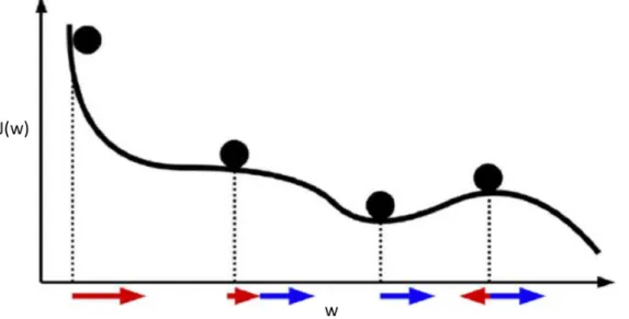
8.2 SGD Process and Influence of Learning Rate. . . 73
8.3 On-line Learning Scenario. . . 74
8.4 Momentum: red arrow represents the direction of gradient, blue arrow represents the direction of momentum. (Source: A. Zhang’s presentation on SASPS [141]) . . . 75
8.5 Nesterov Update Vector. (Source: G. Hinton’s Coursera lecture 6c [131]) . . . 76
9.1 CNN control schema. . . 80
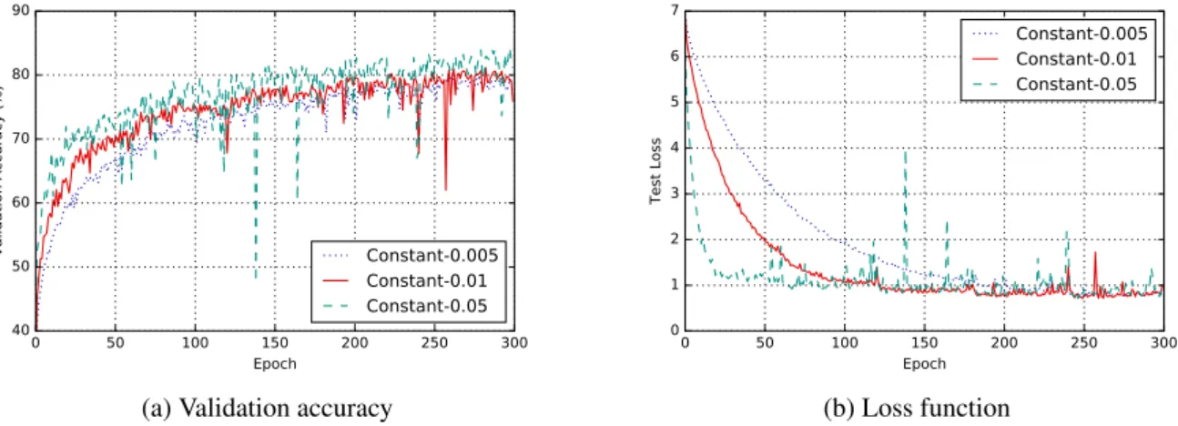
9.2 Impact of different constant learning rates on accuracy and loss (CIFAR-10). . . 81 v
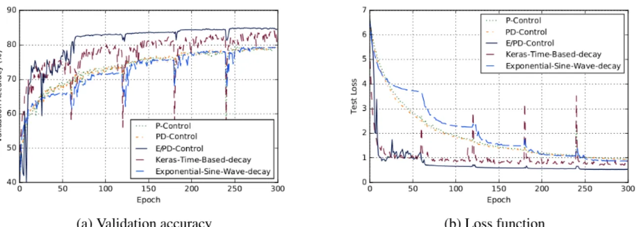
9.3 Performances of state of the art, P, PD and E/PD-Control (CIFAR-10). . . 86
9.4 Control signal of state of the art, P, PD and E/PD-Control (CIFAR-10). . . 86
9.5 Performances of state of the art and E/PD-Control on Fashion-MNIST. . . 87
9.6 Control signal for the state of the art and E/PD-Control on Fashion-MNIST. . . 87
10.1 Event-Based Learning Epochs Continual Learning Scenario. B is the number of data batches, N is the maximum training epochs per batch. . . 94
10.2 E/PD and EB E/PD performance comparison on CIFAR-10 with η(0) = 0.01 initial learn-ing rate. Compact view of the results in Tab. 10.4. . . 97
10.3 Performances of E/PD and EB E/PD on CIFAR-10 . . . 97
10.4 Performance comparison on CIFAR-10 with η(0) = 0.01 initial learning rate. Compact view of the results in Tab. 10.4. . . 98
10.5 Performance comparison on CIFAR-100 with η(0) = 0.01 initial learning rate. Compact view of the results in Tab. 10.5. . . 99
12.1 Noisy Label Data: Incorrectly Label a Tiger as Cat . . . 110
12.2 Co-teaching maintains two networks (A & B) simultaneously. In each mini-batch data, each network samples its small-loss instances as the useful knowledge, and teaches such useful instances to its peer network for the further training. (Source: [59]) . . . 113
13.1 Impact of noisy data on anomaly classification . . . 117
13.2 RAD training data selection framework. Each block is a machine learning algorithm. Data used to train is represented by colored arrows from the top. The flowchart is iterated at every batch arrival with new labelled and unlabelled data coming in (black arrows on the left). The labelled training data for C is cleansed based on the label quality predicted by L. . . 119
13.3 Ensemble Prediction. . . 120
13.4 Evolution of learning over time – Use case of IoT thermostat device attacks. Opt_Sel and No_Sel stand for optimal data selection and no filtering, respectively. _C, _L, and _Ens denote the model or strategy chosen for prediction. . . 122
13.5 Evolution of learning over time – Use case of Cluster task failures . . . 122
13.6 Impact of data noises on RAD accuracy . . . 123
14.1 Impact of noisy data on anomaly classification: Use case of Face Recognition . . . 128
14.2 Structures of RAD and its extensions: four choices of data selection and two choices of prediction technique. . . 131
14.3 RAD - Voting. . . 131
14.4 RAD - Active Learning. . . 132
14.5 RAD Slim. . . 133
14.6 Evolution of learning over time – Use case of IoT thermostat device attacks with RAD Voting and RAD Active Learning (RAD-AL). Full_clean means that no label noise is injected. . . 135
14.7 Evolution of learning over time – Use case of Cluster task failures with RAD Voting and RAD Active Learning . . . 136
14.8 RAD Voting: percentage of hot data and its ground truth. . . 136
14.9 Comparison of RAD Active Learning Limited (RAD-AL-L) and Pre-Select Oracle, show-ing the power of selection. . . 137
14.10Impact of size of initial data batchD0on RAD accuracy with 30% noise level . . . 138
14.12RAD Slim Limited on FaceScrub with 30% noise . . . 139
14.13Unbalanced FaceScrub with 30% noise . . . 140
.1 Utility function of a risk-averse (risk-avoiding) individual. . . 170
.2 Utility function of a risk-neutral individual. . . 171
4.1 Symbol description . . . 28
5.1 ADF test for unit root . . . 44
5.2 VAR lag order selection criterion . . . 44
5.3 Johansen cointegration test . . . 45
5.4 T-test of coefficient in VECM model . . . 46
5.5 Weak exogeneity test . . . 46
5.6 VECM Granger Causality test . . . 47
5.7 Pairwise Granger Causality test . . . 47
6.1 ADF test for unit root . . . 51
6.2 Summary of Output . . . 58
6.3 Summary of Input . . . 61
9.1 CNN configuration . . . 85
9.2 Robustness experiments with varying initial learning rate on CIFAR-10. Mean value (and standard deviation) over 3 runs. The best results are highlighted in bold. . . 88
9.3 Robustness experiments with varying initial learning rate on Fashion-MNIST. Mean value (and standard deviation) over 3 runs. The best results are highlighted in bold. . . 88
10.1 Experiments configuration . . . 95
10.2 Experiments with varying initial learning rate η(0) on CIFAR-10. Mean value over 5 runs are reported. . . 96
10.3 Experiments with varying initial learning rate η(0) on CIFAR-10 and CIFAR-100. Mean value over 3 runs are reported . . . 97
10.4 Double-Event-Based E/PD algorithm experiments with varying initial learning rate η(0) on CIFAR-10. Mean value over 5 runs are reported. . . 100
10.5 Double-Event-Based E/PD algorithm experiments with varying initial learning rate η(0) on CIFAR-100. Mean value over 5 runs are reported . . . 100
10.6 Double Event-Based E/PD experiments on CIFAR-10 and CIFAR-100 in the End of First Round. Mean value over 5 runs are reported. . . 101
13.1 Symbol description . . . 118
13.2 Dataset description . . . 121
13.3 Evaluation of the all algorithms for Cluster task failures datasets and IoT device attacks datasets on 30% and 40% noise level. All the results are averaged on 3 runs. . . 124
14.1 Dataset description . . . 134 viii
14.2 Final accuracy for all algorithms for Cluster task failures datasets and IoT device attacks datasets on 30% and 40% noise level. All the results are averaged on 3 runs. Full-Clean means that no label noise is injected. Opt-Sel means use only clean label data out of all data (mixed with clean and dirty labels). No-Sel means use directly all data. . . 135 14.3 Final accuracy of the different algorithms on FaceScrub dataset with 30% noise, all the
results are averaged on 3 runs. . . 140 .1 Symbol description for Risk Averse . . . 169
1 E/PD-Control . . . 83
2 Robust two-stage training . . . 112
3 RAD . . . 119
4 Ensemble Prediction . . . 120
5 RAD Voting and RAD Active Learning . . . 130
At the time that I finish this thesis, I have spent 21 years of my life in the school. Most of time, I learn from previous studies. But for a PhD candidate, it demands to make original contribution to knowledge: create something new and add some important pieces to the sum of human understand-ing. Even though I cannot be perfect for lots of work, but I have never forgotten these requirements, and it makes me not dare to relax in scientific research. The road to scientific research has never been smooth sailing, just like anything in life. But I am very fortunate to have many mentors and a supporting family. Therefore, I want to dedicate this chapter of thesis to show my gratitude to them.
In the first place, I would like to thank my advisors Bogdan, Louis, Nicolas, Luc and Ioan for their guidance, encouragement, dedication and fellowship. Even though Luc and Ioan are not my official advisors, but from the bottom of my heart, they have no difference from my other three advisors. At the beginning of my PhD, I was just a master student with computer science background. I cannot forget the hundreds of nights that I read the books of economics and control theory, I always have the endless questions. But through all the exchanges of emails and the weekly meetings, I end up as a student that can publish scientific research papers in all above areas. If not for their dedication, motivation and energy, this thesis would undoubtedly never achieved fruition.
I would also like to thank all my collaborators during my PhD. I have the great opportunities to collaborate with Lydia Y. Chen, Robert Birke, Sara Bouchenak, Sonia Ben Mokhtar, Rui Han and Sophie Cerf. They all spent their times to explain their ideas and contributed their works to part of my publications. Without their help, that thesis will never happen.
This work would not have been qualified as a PhD contribution without careful reviews and exam-inations. I thank the jury members Mary-Françoise Renard, Edouard Laroche, Didier Georges, and Guillaume Mercère for the time and expertise they gave during this process.
Research environment is also important to the work. I want to thank all my colleagues in GIPSA-Lab. All the talks we had, all the ideas we shared have all contributed to this thesis. The great help of technical and administrative services plays also an important role for my research in GIPSA-Lab, I want to thank for their help.
PhD is not only a challenge for intelligence, but also a psychological test. I want to thank all my friends for their caring, and of course my parents and my wife for their love and companies. They may never understand what Machine Learning or Macroeconomics talks about, but without their un-conditional and unreserved support and encouragement, I would never have had a chance to start and finish this PhD.
These were the happiest three years I have had, challenging but undoubtedly exciting. Thanks for everyone I met along this journey.
Generalities
Introduction
The first chapter gives a broad outline of this thesis, we introduce the concerned research domains and the topics of the interdisciplinary studies between them. The motivations and contributions are discussed. A reading road-map of this manuscript is provided in the end.
1.1
Context, Motivation and Applications
System identification and machine learning are two similar concepts independently used in auto-matic/econometrics and computer science community. System identification uses statistical methods to build mathematical models of dynamical systems from measured data [124]. Machine learning algorithms build a mathematical model based on sample data, known as "training data", in order to make predictions or decisions without being explicitly programmed to do so [74]. Except the fi-nal prediction accuracy of the model, converging speed and stability are another two key factors to evaluate the training process, especially in the on-line learning scenario, and these properties have already been well studied in control theory. Therefore, this thesis will implement the interdisciplinary researches between these areas.
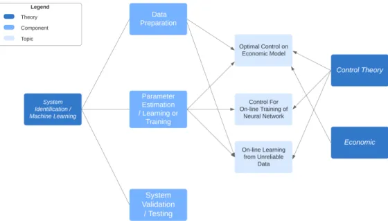
The conducted studies can be divided into three topics, Fig. 1.1 illustrates the main concerned domains for each topic of studies. In general, the process of system identification / machine learning, can be summarized to three steps: 1) data preparation, 2) parameter estimation / learning or training and 3) system validation / testing. The second step is just one concept, two statements, and the main difference is in the third point. For some applications of system identification, especially the model-driven applications, use the same training data to valid the model (examples in chapter 6 in [80]), while machine learning algorithm specifically prepares a testing dataset to evaluate the prediction accuracy. The main contributions of this thesis are on the first two steps, where we incorporate control theory into these steps to improve the performance under certain circumstances.
The first topic is optimal control on economic model. Obviously, this topic consists of two parts: 1) system identification and 2) optimal control. Economists develop economic models to explain con-sistently recurring relationships [19]. E.g., the optimal growth model: Solow-Swan model [125, 127], which studies long-run economic growth by looking at capital accumulation, labour or population growth, and increases in productivity (commonly referred to at technological progress). And Ramsey-Cass-Koopmans model [109, 22, 73] that analyses the consumer optimization, endogenizing the sav-ing rate while take interest rate and discount rate into consideration. Econometrics is the tool to con-duct these analysis (dynamic optimization technique is used). Econometrics uses economic theory, mathematics, and statistical inference to quantify economic phenomena. In first part of this topic, we first present an analysis which uses only method from econometrics on China macroeconomic data. This work is not only a good practice for us (who with the background in automatic and computer
Figure 1.1 – Mainly concerned domains for the topics of study
science) to understand the theories used in econometrics, but also make the contributions in economic area, to reveal the trend of China’s economic growth transition: from export-oriented to consumption-oriented. In second part of this topic, we perform the system identification on France macroeconomic data with Vector AutoRegressive (VAR) framework with Least Squares (LS) estimation, the identi-fied model is presented in the favour of control, which means the model is represented on state space form. In economic area, there are studies to discuss extending VAR framework to analyze scenarios with unobservable explanatory variables by using state space models [78, 136, 84], because when explanatory variables are not observable, LS estimation is not usable. However, one can apply like-lihood based inference, since the so-called Kalman filter allows to construct the likelike-lihood function associated with a state space model. Except dynamic linear models with unobserved components, many other dynamic time series models in economics can also be represented in state space form, for instance, 1) autoregressive moving average models or 2) time varying parameter models [40]. In our case, the reason to use state space form instead of autoregressive equation is because it is easier to design the optimal controller via Linear Quadratic Regulator (LQR) solution. The LQR algorithm is essentially an automated way of finding an appropriate state-feedback controller. Once the model is estimated, the control system can apply the control law to bring the system to the desired state (e.g. a 3% yearly constant growth rate of Gross Domestic Production (GDP) in the macroeconomic model). We can also impose perturbations on outputs and constraints on inputs. This simulation can closely emulate the real world situation of economic crisis (e.g. 2008 financial crisis and Covid-19 pandemic). And economists can observe the recovery trajectory of economy with limited resources, which gives meaningful implications for policy-making. Control theory has been successfully imple-mented in economic domain to cope with problems such as: monetary policy [20, 62], fiscal policy [90] and resource allocation [29, 66]. Our work makes the contributions to expand it to macroeco-nomic models.
The second topic talks about using control theory to improve the on-line training of neural net-work. For on-line training scenario, training data comes in batches. One challenge of this setting is that the time interval between two data batches may be short, so we need the model to learn as quickly as possible. Another uncertainty is that the data distribution between different data batches may be very different, and we need to ensure that the model continues to improve. Learning rate and gradient are two main factors to control the converging speed, the state of the art learning rate algorithm can
be grouped into two categories: 1) time-based and 2) adaptive gradient. The time-based method pre-fixes a trajectory of learning rate before training process, no matter it is monotonous decreasing [26], decreasing with sine wave oscillation [2] or cyclical changing [123] over time. The advantage is easy to adopt, but the disadvantage is that the learning rate can not be adjusted even for some data batches, we could (should) certainly have a bigger (smaller) learning step. Adaptive gradient method such as Adam [72] is recent state of the art, but research [138] suggested that adaptive gradient methods do not generalize as well as stochastic gradient descent (SGD). These methods tend to perform well in the initial portion of training but are outperformed by SGD at later stages of training. Even though the algortihms such as AmsGrad [111] and AdaBound [89] claimed they fixed the defects in Adam by their method (see Sec. 8.4.2), but their results tested under on-line learning scenario do not show advantages (see Sec. 10.3). Therefore, we propose our performance-based learning rate algorithm: E (Exponential) / PD (Proportional Derivative) feedback control. Training a neural network is the pro-cess to minimize the cost function, i.e. minimize the loss value, in our designed control system, we represent the Convolutional Neural Network (CNN) as plant, the learning rate as control signal and the loss value as error signal. The experiments are based on CIFAR10 [76] and Fashion-MNIST [139] datasets, the results show that not only our algorithm outperforms the comparisons in final accuracy, final loss and converging speed, the result curve of accuracy and loss are also extremely stable near the end of training.
Still for the second topic, one observation from E/PD experiments is that when the loss value continuously decreases, our learning rate decreases too. But as the loss continuously decreases, it means we are in the good direction of training, we should not decrease the learning rate at that time. To prevent this sudden drop of learning rate at PD phase, we propose an event-based learning rate algorithm based on E/PD: Event-Based Learning Rate. Results show that event-based E/PD improves original E/PD in final accuracy, final loss and converging speed. Even the new algorithm introduces small oscillations to the training process, but the influence is minor.
Another observation from E/PD experiment is that on-line learning fixes a training epoch number for each data batch. But as E/PD converges really fast, the significant improvement only comes from the beginning epochs for each data batch, the latter ones do not have much contributions for the training. Therefore, we propose another event-based control based on E/PD: Event-Based Learning Epochs, which inspects the historical loss value, when the progress of training is lower than a certain threshold, we pass the current data batch, turn to welcome the next batch. The experiments are based on CIFAR10 and CIFAR-100 [76] datasets. Results show that event-based learning epochs can save up to 67% epochs on CIFAR-10 without degrading much model performance.
The third topic focus on noisy (dirty) label data learning problem. This topic retraces to a fun-damental assumption in system identification and machine learning: the data source is clean, i.e., features and labels are correctly set. But big data are everywhere in research now, and the data sets are only getting bigger, which makes it challenging to ensure the data quality. In this part, we only consider the noise on data labels instead of on data features. Considering noisy data in classifica-tion algorithms is a problem that has been explored in the machine learning community as discussed in [44, 14, 101]. And our motivating case studies (Sec. 13.2 and . 14.2) also show that noisy label data can degrade the performance of machine learning algorithms. To tackle this problem, we propose a generic framework: Robust Anomaly Detector (RAD), RAD is a framework that model within RAD can continuously learn from dirty label data. It is called anomaly detector is because we implement this framework for anomaly detection purpose in our analysis, but its usage is not limited to anomaly detection. The data selection part of RAD is a two-layer framework, where the first layer is primarily used to filter out the suspicious data, and the second layer mainly detects the anomaly patterns from the remaining data. With our designed ensemble prediction, predictions from both layers contribute to the final anomaly detection decision. Two experiments are conducted on two datasets: 1) IoT device
attack detections 2) Google Cluster task failure predictions. And the training scenario is also setting to on-line learning scenario, a small difference is that the on-line learning in this part trains the model with all accumulated data instead of only latest data. Results show that RAD can continuously im-prove model’s performance under the presence of noise on labels, comparing to the scenario without filtering any noisy label data. And the experiment with varying noise level shows that RAD can resist on high noise level.
RAD indeed improves the result with noisy label data, but it is not flawless. One shortcoming is that we use only first layer model to do the data selection, meanwhile we train two models simul-taneously. We should include second layer to do the data selection too. As for that, we propose a new framework RAD Voting, the difference is that RAD Voting selects training data based on the conflict of predictions from two models. Also as we observed from RAD experiment, the models are improving over time, RAD Voting uses thus current model to re-select the training data from old data batches to improve training data quality. Results show that RAD Voting outperforms RAD in final accuracy.
In the end of topic three, we introduce another extension of RAD: RAD Active Learning, which we introduce an expert in the framework, the data selection part is similar as in RAD Voting, but when there is conflict on the prediction of two models, these uncertain data will send to expert, and expert will return the ground true labels of these data. The experiment results are very promising, the RAD Active Learning performs almost as good as the case where there is no noise on labels.
This section briefly introduced the motivations and main contributions in this thesis, the detail of related work for each topic are given at the beginning of Part. II III and IV, respectively. The very detailed motivations and contributions are presented in Sec. 2.4 and 3.2. Part. V draws conclusions on this work and provides insights of future works that would worth investigating on.
1.2
Main Results and Collaborations
1.2.1
Publications
The work developed in this thesis has lead to several contributions which have been published in various venues, both the control and computing systems communities. All my works have been partially supported by the LabEx PERSYVAL-Lab (ANR-11-LABX-0025-01) funded by the French program Investissement d’avenir.
International Journals
• Zilong Zhao, Sophie Cerf, Bogdan Robu, Nicolas Marchand. Event-Based Control for On-line Training of Neural Networks IEEE Control Systems Letters (L-CSS), vol. 4, no. 3, pp. 773-778, July 2020. [145].
• Minor revision: Zilong Zhao, Sophie Cerf, Bogdan Robu, Nicolas Marchand, Sara Bouchenak. Enhancing Robustness of On-line Learning Models on Highly Noisy Data. IEEE Transac-tions on Dependable and Secure Computing (TDSC), Special Issue: Artificial Intelligence/Machine Learning for Secure Computing
• Submitted: Zilong Zhao, Louis Job, Luc Dugard, Bogdan Robu. Modelling and dynamic analysis of the domestic demand influence on the economic growth of China. Review of Development Economics
• TBD: Zilong Zhao, Bogdan Robu, Ioan Landau, Nicolas Marchand, Luc Dugard, Louis Job Modelling and Optimal Control of MIMO System - French Macroeconomic Model Case. TBD
International Conferences
• Zilong Zhao, Louis Job, Luc Dugard, Bogdan Robu. Modelling and dynamic analysis of the domestic demand influence on the economic growth of China. Conference on International Development Economics, Nov. 2018, Clermont-Ferrand, France [146]
• Zilong Zhao, Sophie Cerf, Robert Birke, Bogdan Robu, Sara Bouchenak, Sonia Ben Mokhtar, Lydia Y. Chen. Robust Anomaly Detection on Unreliable Data. 49th IEEE/IFIP International Conference on Dependable Systems and Networks (DSN 2019), June 2019, Portland, Oregon, USA [142]. (acceptance rate: 21.4%)
• Zilong Zhao, Sophie Cerf, Bogdan Robu, Nicolas Marchand. Feedback Control for On-line Training of Neural Networks. 3rd IEEE Conference On Control Technology And Applica-tions (CCTA 2019), Aug. 2019, Hong Kong, China [143].
• Amirmasoud Ghiassi, Taraneh Younesian, Zilong Zhao, Robert Birke Valerio Schiavoni,
Ly-dia Y. Chen. Robust (Deep) Learning Framework Against Dirty Labels and Beyond.
2019 IEEE International Conference on Trust, Privacy and Security in Intelligent Systems and Applications (TPS-ISA), Dec. 2019, Los Angeles, California, United States. [48].
1.2.2
Collaborations
Those works has been conducted thanks to fruitful collaborations:
• Pr. Ioan D. Landau (Gipsa-lab, Univ. Grenoble-Alpes) on system identification and control, • Pr. Luc Dugard (Gipsa-lab, Univ. Grenoble-Alpes) on system identification and control, • Dr. Lydia Y. Chen (TU Delft) on dirty label data learning and active learning,
• Dr. Robert Birke (ABB Research) on dirty label data learning,
• Pr. Sara Bouchenak (LIRIS lab, INSA-Lyon) on dirty label data learning, • Dr. Sonia Ben Mokhtar (LIRIS lab, INSA-Lyon) on dirty label data learning, • Dr. Rui Han (Beijing Institute of Technology) on dirty label data learning, • Dr. Sophie Cerf (INRIA) on dirty label data learning and event-based control,
1.2.3
Technical contributions
The contributions of the above publications are not only on theoretical area, technical advances are also made.
• During the preparation for the economic method, we have developed a Ramsey–Cass–Koopmans model simulator1 based on a matlab project2. All the code are realised in matlab, the interface is developed by Simulink.
• The learning rate algorithm proposed in [143] and [145] are published as open-source code in github3. The E/PD control and the event-based learning rate and event-based learning epoch controls are all packaged as learning rate scheduler in Keras1[26] library, which make users very easy to adopt to their own projects.
1video demo: https://www.youtube.com/watch?v=iXP0kQ9hig0
2project link:
https://www.mathworks.com/company/newsletters/articles/simulating-the-ramsey-cass-koopmans-model-using-matlab-and-simulink.html
• The framework RAD which is proposed to learn from unreliable data is developed in python with scikit-learn [105] and Keras libraries. The code of vanilla RAD is published on github4. As the paper for extension of RAD is still under review, we will publish the code later under this git5.
• The optimal control framework developed for french macroeconomic model will also be pub-lished in the same git account as RAD. The framework is coded in Simulink. Since the paper is not published yet, the code remain confidential for now.
1.3
Thesis Outline
This thesis consists of five parts. The first part gives a general overview of the background, motivation and contributions of the works. From the second to the forth part, we elaborate the conducted stud-ies in three topics: 1) System identification and optimal control on Macroeconomic data, 2) Control theory for on-line training of neural networks and 3) On-line learning from highly unreliable Data demonstrated on the use case of anomaly detection. The fifth part concludes on the whole contribu-tions of this thesis, and gives possible direccontribu-tions for future works. Each part is divided in chapters, the content of each chapter is briefly described as follows.
Part 1 - Generalities.
Chapter 1 - Introduction. First chapter introduces the context of the all three research topics, their background, and an general picture of the main results achieved. Publications, collaborations and technical contributions through all the works in this thesis are also given in this chapter. The outline of this thesis and the read road-map for readers from different academic background are provided in the end.
Chapter 2 - Background and Motivation. This chapter elaborates the basic ideas of control theory, system identification and machine learning, which are the three research domains we explored in this thesis. It shows the objective of control system and how it works, and provides the comparisons between system identification and machine learning. Motivating cases are showed in this chapter, which leads to our following research in Part. II III and IV.
Chapter 3 - Objectives and Contributions. This chapter sets forth the objectives of the research topics in Part. II III and IV, which is mainly the responses to the motivating cases discussed in Chapter. 2, and explains the theoretical and technical contributions of the works from each topics. Part 2 - System Identification and Optimal Control on Economic Data.
Chapter 4 - Background on System Identification and Control. This chapter first introduces two optimal growth models: 1) Solow-Swan model and 2) Ramsey-Cass-Koopmans model. These two models are not used in later context, but they are giving the ideas how do economists apply optimal control on economic problem. Then we introduce the background of system identification methods used in econometrics, such as Augmented Dickey-Fuller test for verifying the stationarity of time series, or Vector Autoregressive Exogenous (VARX) model to modelize the macroeconomic data. The background of system identification in automatic is also introduced, such as state space representation. And one optimal control solution: LInear-Quadratic Regulator (LQR) is also presented.
Chapter 5 - Modelling and Dynamic Analysis of the Domestic Demand Influence on the Economic. This chapter presents an economic study on China macroeconomic data. Comparing
4project link: https://github.com/zhao-zilong/RAD
to previous studies, we include the time series from recent years, and add more variables into the models. Econometrics methods are implemented to identify the economic model, Granger causality tests are conducted between the economic growth, household final consumption, inward foreign direct investment and export in China. The experiments are realised on Eviews.
Chapter 6 - Modelling and Optimal Control of MIMO System - French Macroeconomic Model Case. After identifying the macroeconomic model of China with econometrics methods, this chapter uses France macroeconomic data, and represent the study in an automatic way. We regard the model as a Multiple-Input and Multiple-Output (MIMO) system, and represent the model in state-space form, which can help to design the controller. The optimal controller is designed via Linear-Quadratic Regulator (LQR). The experiments are conducted with different parameters of LQR, and perturbations on outputs and constraints on inputs. The system identification experiments are realised on Gretl and Matlab. The control system is illustrated on Simulink.
Chapter 7 - Conclusion on Economic Model Control. This chapter summarizes Part. II, con-cludes their results and gives perspectives on future works.
Part 3- Control Theory For On-line Training of Neural Networks.
Chapter 8 - Neural Network and Learning Rate: Background and Related Works. This chap-ter introduces the Convolutional Neural Network structures, the performance metrics to evaluate the neural network and Continual (On-line) learning scenario for Part. III. It details different type of time-based learning rate algorithms, and elaborates the state of the art adaptive-gradient methods.
Chapter 9 - Exponential / Proportional-Derivative Control of Learning Rate. This chapter introduces the performance-based learning rate algorithm: Exponential (E) / Proportional-Derivative (PD) control. This study is mainly compared with time-based learning rate methods. It first shows some motivation cases from fixed learning rate scenario, and gradually presents the P, PD and E/PD control. The experiments are on two image datasets: CIFAR-10 and Fashion-MNIST. All the exper-iments are realised based on Keras (tensorflow backend) library, with the help of GPU from google cloud compute engine.
Chapter 10 - Event-Based Control for Continual Training of Neural Networks. Based on E/PD control, this chapter introduces two event-based control to improve E/PD in continual learning scenario: i) Event-Based Learning Rate and ii) Event-Based Learning Epochs. The experiments are conducted on CIFAR-10 and CIFAR-100, and the results are compared with four state of the art adaptive gradient method: 1) Adam 2) Nadam 3) AMSGrad and 4) AdaBound.
Chapter 11 - Conclusion on Learning Rate Control. This chapter concludes the Part. 9, gives the possible direction to extend this work.
Part 4- On-line Learning from Highly Unreliable Data: Anomaly Detection.
Chapter 12 - Noisy Data Learning and Anomaly Detection: Background and Related Works. This chapter introduces the problems of noisy data learning and anomaly detection. It details the features of the anomaly detection datasets that we will deal with. The different continual learning setting for different datasets is presented, and the previous state of the art algorithms that we will compare with are illustrated with formula and schema.
Chapter 13 - Robust Anomaly Detection on Unreliable Data. Robust Anomaly Detector (RAD) is a generic framework to deal with the dirty label data learning problem, it is called anomaly detector is because it is first applied to deal with anomaly detection problem. This chapter presents the RAD with our designed ensemble prediction method. The evaluations are based on two dataset: 1) IoT thermostat device attack detection and 2) Google cluster task failure prediction. In the end of evaluation, the limitation of RAD is discussed. The experiments are implemented with Scikit-Learn library.
Chapter 14 - Extension of RAD framework for On-line Anomaly Detection for Nosiy Data. Due to the limitation of RAD presented in Chapter. 13, we propose several extensions of RAD to improve these deficiencies. RAD Voting and RAD Active Learning are two enhanced version of RAD based on the additional features of conflicting opinions of classifiers, repetitively cleaning, and oracle knowledge. To show the broad applicability of RAD (and its extensions) framework, we extend the evaluation with a new dataset FaceScrub, which is to recognize 100 celebrity faces. RAD Slim is an adapted version of RAD Active Learning for image dataset. The experiments are implemented with Keras and Pytorch libraries in this chapter.
Chapter 15 - Conclusion on Noisy Data Learning. This chapter concludes the studies for the topic of noisy data learning, and provides insights for future works.
Part 5- Conclusions and Perspectives.
The ending part of this thesis is dedicated to conclude the whole contributions from Part. II III and IV. By analysing the results, we point out some theoretical improvement directions for certain studies, and possible experimental extensions for current work.
1.4
Read Roadmap
Since this thesis touches various research domains, this section guides the readers from different backgrounds or with different interests.
For the reader with interest in Economics. The whole Part. II is dedicated to discuss the eco-nomic problem. If one has ecoeco-nomic background, there is no difficulty to understand the Chapter. 5 which studies the economic transition of China. Chapter. 6 also focuses to analyze economic data, it incorporates french macroeconomic model into the control system to conduct optimal control. There-fore for the reader without control knowledge, one has to at least read the Sec. 2.1 and Sec. 4.2 to understand the basic of control system and optimal control.
For the reader with interest in applications of Control Theory. Chapter. 6 applies optimal control (designed via LQR) on economic model, simulation with 1) varying parameter of LQR, 2) constraints on inputs and 3) perturbations on outputs are implemented. Part. III explores to integrate control theory into learning rate algorithm of machine learning. Chapter. 9 proposes a performance-based feedback control E/PD, which updates the learning rate performance-based on the evolution of historical loss value. Chapter. 10 two event-based controls: i) event-based learning rate and ii) event-based learning epochs. First is used to improve E/PD, second one is used to reduce the inefficient training epochs. Even though these controls are used to improve machine learning algorithms, all the studies in Part. III have been published in conference and journal of control community, therefore their presentations are in favor of the reader with control background. E/PD and event-based learning rate are also involved in the experiments in Chapter. 14 for RAD Slim algorithm, but they are only implemented to accelerate the training process, not theoretical innovations of these algorithms in that part.
For the reader with interest in Machine Learning. Part. III is dedicated to improve the machine learning algorithm performance under continual learning scenario. Since the achievement is realised with control theory. It is better for the reader without control background to read Sec. 2.1 first, to have an impression of the control system and feedback control. Part. IV is quite independent, readers who are interested with dirty label data training problem, can skip other chapters.
Background and Motivation
This chapter gives a general overview of Control Theory, System Identification and Machine Learn-ing. First, basic concepts are explained as an attempt to depict the global picture of the field, as well as to give a rapid introduction for readers unfamiliar with the terminology. Then, motivation cases associated with control theory, system identification and machine learning are discussed.
2.1
Basics of Control Theory
Control theory is a theory that studies how to adjust the characteristics of dynamic systems. The process under study should evolve over time and be causal (only past and present events impact the future). Fig. 2.1 presents a system (physical, biological, economic, etc., referred usually as plant) in control community. In this schema, at least one of the outputs should be able to measure, and at least one of the inputs can influence the outputs through the configuration of the plant. The plant can be characterised using the mathematical model which contains a set of parameters that describes its behaviors. For time-variant system, the parameters of the model can change over time, and for time-invariant system, we assume these parameters are fixed during the whole time. Depending on number of inputs and outputs, a system can be either SISO (Single-Input, Single-Output), MIMO (Multi-Inputs, Multi-Outputs) or a combination of the two.
To sum-up, a system eligible for control should be dynamic, causal and be configurable by at least one input signal, and observable with at least one output signal [53].
Figure 2.1 – Representation of system in control
Given such a system, three complementary goals can be achieved when using control theory [23]: • Stability. There are three type of stability in control theory: 1) The stability of a general dynamical system with no input can be described with Lyapunov stability criteria. That is, any trajectory with initial conditions around x(0) can be maintained around x(0); 2) A linear system
is called bounded-input bounded-output (BIBO) stable if its output will stay bounded for any bounded input; 3) Stability for nonlinear systems that take an input is input-to-state stability (ISS), which combines Lyapunov stability and a notion similar to BIBO stability. In this thesis, we mainly focus on the second case BIBO stable. Control can be used to stabilize an unstable system, but most of all it should ensure to keep stable an originally stable one.
• Tracking. Once the system is ensured to be stable, one may consider the behavior of the plant. One main objective of control system is to let the output of plant follow our desired trajectory. There are several indexes to evaluate a controller. Assume the reference is a constant signal, one index is the precision, which means how close the output and reference. Another index is the responsetime which represents the time from beginning to the moment output is stable. Overshoot is also an important index, it measures the maximum value above reference.
• Disturbance Rejection. As no system evolves in a perfectly mastered environment, a control strategy should be able to deal with exogenous influences. Whether these disturbances can be measured or not, modeled or not; control theory provides ways to reject them, i.e. mini-mize their impact on the plant outputs. This aspect of control is called a perturbation rejection problem.
2.2
Feedback Control
A control system can be regarded as a system with four functions: (i) Measurement, (ii) Comparison, (iii) Calculation and (iv) Correction. As open loop control strategies are not used in this thesis, we focus on closed loop (also referred to as feedback) control system in this section. A high-level representation of a feedback control system can be illustrated in Fig. 2.2. It introduces three extra elements comparing to system in Fig. 2.1: (1) a reference signal; (2) a controller (containing a control algorithm); (3) a feedback from output to input. The output (i.e. measurement) signal is compared to its reference, to which the plant should tend. The difference between the reference and the output is used as input (referred to as error in Fig. 2.2) for controller to generate a control signal. The idea behind this design is easy to understand, if the error is big, we need to largely adjust our control signal to stimulate the plant, so that the output quickly approaches to the reference. If the error is small, we should carefully adjust the control signal. The objective of this control system is to minimize the difference between the reference and the output.
The control engineer usually uses the imperfect knowledge of the plant (represented as a state space or transfer function) to compute the controller algorithm which will make the closed loop plant comply with the functionality and technical specification.
2.3
Basics of System Identification & Machine Learning.
The field of system identification uses statistical methods to build mathematical models of dynamical systems from measured data [124]. The term system identi f ication is mainly used in the field of control engineering.
Machine learning (ML) is the study of computer algorithms that improve automatically through experience [97]. Machine learning algorithms build a mathematical model based on sample data, known as "training data", in order to make predictions or decisions without being explicitly pro-grammed to do so [74, 17]. The term machine learning is mainly used in computer science field.
We can see that both notions build mathematical models, they all try to use available historical data to approximate the function (relation) between input and output. The main difference between these two notions reside in the usage. While some of system identification algorithms care more if the estimated model fits well the training data (e.g. model-driven estimation), in order to build an efficient algorithm. Machine learning cares more if the estimated model can predict well in the new data. That is why machine learning is also referred to as predictive analytics.
The procedure of performing the system identification and machine learning are almost same. The high-level steps to perform system identification and machine learning on a dataset can be summarized as showed in Fig. 1.1: 1) Data Preparation, 2) Parameter Estimation / Learning or Training, and 3) System Validation / Testing.
• Data Preparation. When we deal with a dataset, we almost never use the original data to estimate the model. For instance, the stationarity is important if we do the regression on time series. If the time series are non-stationary, the regression gives spurious results (see Part. II). The cleanness of training data is vital for training machine learning model, if the collected data are polluted, the true output yi of input xi is not reliable, the trained model can be corrupted
(see Part. IV). To solve above problems, we need to deal with the data before feeding data to algorithm.
• Parameter Estimation / Learning or Training. The parameter estimation in automatic control is similar to the term of Learning or Training for machine learning. It is the process to approx-imate the functions between input and output by mathematical methods. For linear regression, Ordinary Least Square (OLS) and Maximum Likelihood Estimationis (MLE) are widely used. And for more complex task such as face recognition, neural network is the common choice, then convolution and gradient (Sec. 8.1) are necessary.
• System Validation / Testing . The main difference between System Identification in automatic and Machine Learning in computer science is in this step. For system identification, to validate the estimated model, we use the data which is used to train the model to test the model. The aim is to check if the model has perfectly fitted on the data. If the residuals from the validation are white noise, we believe the estimated model is good. In machine learning, before training the model, we need to split the whole dataset into one training dataset and one testing dataset. The ratio between testing and training dataset is often 1:2 or 1:3. Only training dataset is used to train the model, and only testing dataset is used to test the model.
Above three points are only high-level skeleton of the pipeline, there are also other details when we implement. For example, if we perform the auto-regression on time series, before estimating pa-rameters of model in parameter estimation step, we need to estimate the order of model first, this part is discussed in Sec. 5.4 and Sec. 6.2.2. Estimation of model’s order can help to build a model with least parameters but still valid. This step as well as model order reduction usually does not appear in machine learning, one reason can be the interpretability of the model, from the highly interpretable
lasso regression to impenetrable neural networks, but they generally sacrifice interpretability for pre-dictive power. Since many of the model’s structures are unexplainable, it will be difficult to justify any reduction of the model.
2.4
Motivation Cases
In this section, we provides some real world cases which motivate us to perform our studies in fol-lowing three parts.
2.4.1
Control Theory on Macroeconomic Model
First, let us check the quarterly GDP growth rate from 2005Q1 to 2018Q1 in Fig. 2.3. EA denotes to Euro Area. EU and US denote to European Union and United State. One can observe a big drop around 2008Q4 and 2009Q1, which is the period of the 2008 financial crisis. If we see the macroeconomic system as the plant we introduced in Sec. 2.1, then GDP can be modelized as one of the outputs. In macroeconomic, we know there are several economic variables we can control, for instance the interest rate in central bank, the oil price, the public expenditure from government, etc. We can see these variables as the inputs of the plant, then we can easily modelize the economic crisis problem as control problem. We can also add perturbations on outputs, constraints on inputs. By simulating the system, we can emulate different kind of crisis on different outputs. Observing the reaction of inputs during the system recovery process provides very good political implications for economists to study. This study is explored in Part. II.
Figure 2.3 – Quarterly GDP Growth Rate from 2005Q1 to 2018Q1 (Source: Eurostat)
2.4.2
On-line Training of Neural Network
On-line training (or continual learning) is widely used in many scenarios, when there is not much available data at beginning. For example shopping site or Netflix, when a new user comes in, there is no historical information of the user, then the recommended products or films are not well fitted to user’s taste. As the user generates more data, the recommendations are more accurate.
There are two scenarios of on-line learning setting: 1) the size of data is relatively small, every time a user generates new data, we can retrain the model with all accumulated historical data. 2) if the size of data is large, when there is newly generated data available, we can only use the new data to train the model instead of re-learning with all the accumulated data.
Apart from the data size, time interval of data generation is another factor to consider, it challenges the convergence speed of algorithm. Learning rate and Gradient are two key parts which influence the convergence speed of machine learning algorithms. After studying the previous strategies, they can be summarized as: (1) time-based learning rate, (2) adaptive gradient. The problem of time-based method is that its learning rate is prefixed before training process, which makes it impossible to react, even though sometimes it can accelerate the learning speed as we are far from optimum, or slow down the learning speed as we are close to the optimum in case we do not skip it. For adaptive gradient methods, there are studies show that adaptive gradient methods do not generalize as well as stochastic descent gradient (SGD). These methods tend to perform well in the initial portion of training but are outperformed by SGD at later stages of training.
Above studies drive us to think: If we can develop a performance-based learning rate algorithm using SGD? So that we can overcome the shortcomings in time-based learning rate and adaptive gradient methods. The performance-based controller can be designed to solve this problem.
Actually the following thoughts come out after we finished the performance-based controller. For a typical machine learning setting, we need to fix a number of training epochs before we launch the training process. Since we developed the performance-based controller, the converging speed of the model is largely accelerated, and as the algorithm is already converged after several epochs in the beginning, the following training epochs becomes less useful. This phenomenon drives us to propose an event-based control to decide when we stop the learning, that will shapely reduce the training epochs while maintaining a good model. Above studies are performed in Part. III.
2.4.3
Dirty Label Data Learning
When we try to build a specific image classification model, the first step is to prepare a labelled dataset. There are several ways to get high-quality labelled data, for example, explore pre-labelled public datasets or leveraging the crowd-sourcing service. But in most case, we need to harvest our own training data and labels from free sources. Here we illustrate the struggles one can experience when construct their own dataset and explain why we need to solve this problem.
Imagine one wants to build an image classification model to distinguish if an image is airplane, and we assume that there is no free available pre-labelled public datasets. Then the fastest way we can think about is to use google. If we search keyword "airplane" in Google image search, the first pages will show the images as in Fig. 2.4. There are different type of airplanes, and this is what we want to collect.
(a) (b)
In reality, if we want to quickly gather as many as possible the images, one useful tool is the web crawler, it will help us to thousands of images by running a few lines of code instead of downloading them one by one by clicking. However, if we check the later pages of google results, other relevant images pop up. For instance, the images showed in Fig. 2.5 are the cabinet of airplane and a cartoon image of an airplane. To solve this problem, one can manually check all the images. But when the dataset is huge, that can be really time consuming or even impossible. That motivates us to propose a proper algorithm to address this problem to mitigate the influence of dirty labelled data on final classification model.
(a) (b)
Objectives and Contributions
In this context of association of control theory, system identification and machine learning, this thesis explores the problems which can be grouped into three subjects which will be presented in Part. II, III and IV. The main objective of this thesis are detailed as follows:
3.1
Objectives
Part. II focuses on the problem of system identification and optimal control of the macroeconomic model, the study is based on the economic data from China and France. In this study, we will show the methods used in Economics and Automatic to perform the system identification. After that, we will show two use cases on how economists achieve optimal growth for economic models (Solow-Swan model and Ramsey-Koopmans-Cass model). And then we will introduce our designed optimal control model, one advantage of our algorithm is that it can take into account of constraints on inputs and the state of the system as well as perturbations on outputs .
Part. III incorporates control theory into learning rate algorithms, aiming to accelerate the ma-chine learning process on continual learning scenario. The state of the art algorithms can roughly be divided into two categories: i) time-based learning rate, and ii) adaptive gradient learning rate. The algorithms from these two groups all have their own drawbacks. Time-based learning rate can not adjust its learning rate regards to the training data and training phase, which leads to a slow con-verge speed of the training process. Adaptive gradient methods performs better in concon-verge speed comparing to time-based learning rate, but its final accuracy tends to be worse than the method based on the stochastic gradient descent (SGD). Therefore, we propose a performance-based learning rate algorithms, which not only converge as fast as (or even faster) the adaptive gradient methods, but also ensure no compromise on final accuracy as it is based on SGD. Besides the performance-based learning rate, we also propose an event-based control algorithm which aims to automatically decide when the training process stops and forwards to next training batch in continual learning scenario. To massively cut off inefficient training epochs but still accelerate the learning process.
Part. IV sheds light on dirty label data problem, which means that, as the training data quality is difficult to be guaranteed, we design the algorithms to alleviate the influences of dirty label data on the model. The algorithms are compared with several state of the art, in respect of final accuracy, final loss value, converging speed and stability of the performance. The experiments are implemented on three datasets: 1) IoT device attack detection, 2) Cluster task failure prediction and 3) face recognition, in order to show the board applicability on different type of data.
3.2
Contributions of the Thesis
In this section, we will summarize the contributions of this thesis from each chapter that presented in Part. II, III and IV.
3.2.1
Dynamic Analysis of China Macroeconomic Model
This study uses the classical economic methods to perform system identification, comparing to pre-vious researches, we extends the time series with recent year data, include new variable: Household Consumption into the macroeconomic model. We also implement tests to show the Granger causal-ities between variables. Many studies on the early stage of Open Door Policy have shown that there are two-way Granger causalities between Export, FDI (Foreign Direct Investment) and GDP (Gross Domestic Production), but our study shows that with recent year data, the growth of FDI and the growth of GDP have no two-way Granger causalities any more, but the growth of Consumption does.
3.2.2
Optimal Control on France Macroeconomic Model
This study is based on France’s macroeconomic data, we perform the system identification as we typically do in Automatic. After estimating the model, the optimal control solution: LQR is designed for our problem which is to maintain a constant GDP increasing ratio. And once the system is stable, we introduce the perturbations on all outputs (i.e. IMP. EXP, GDP). Introducing shock on variables in VAR has been well studied in economic area by impulse response function (IRF). IRF traces the ef-fects of an innovation shock to one variable on the response of all variables in the system. Comparing to IRF, our approach not only observes the changes after the shock, but also intervenes the process of recovery. Our objective is to use all the available resources to help the model regain the stability, re-turn to the level before the shock. We also impose the constraints on inputs, all these factors together help us to well emulate the real world situation (e.g. 2008 financial crisis and Covid-19 pandemic). The whole control system is realised with Simulink (a handy simulating environment), we think this tool can help economist to better estimate the recover trajectory of the economy.
3.2.3
Exponential / Proportional-Derivative Control of Learning Rate
When performing image classification tasks with neural networks, often comes the issue of on-line training, from sequential batches of data. The interval between data batch can be short and the data distribution from one batch to another can vary a lot. All these problems lead us to design a better algorithm, which can make the training process converge faster so that we can reduce training time, and the algorithm should also be stable when we change the data batch from one to another. In addi-tion to that, our algorithm should not sacrifice its final accuracy and final loss for maintaining stable and faster converging speed. That is why we propose a performancebased learning rate algorithm -Exponential (E) / Proportional-Derivative (PD) control, it converges faster than the compared state of the art algorithm, it’s much stable than others near its end of training, and its final accuracy and loss is lower than the comparisons.
3.2.4
Event-Based Control for Continual Training of Neural Networks
This work is an extension work based on E/PD control we mentioned in last section. We first propose an enhanced version of E/PD - Event-Based E/PD. It can prevent the learning rate to decrease when loss value continuously decreases. The result shows that this small change indeed improves the model in all the index we mentioned in last section.
We also propose a second event-based control based on E/PD, this control is based on our ob-servation that when we implement E/PD on continual learning scenario, the significant improvement in the learning only occurs at the beginning when loading a new batch, the accuracy and loss value evolve slowly afterwards. Therefore, we implement an event-based control to inspect the record of the loss value. If the loss record has the tendency to increase, showing little learning efficiency, we will drop the rest learning epochs for current data batch. In the experiment with dataset CIFAR10, it could save up to 67% training epochs.
3.2.5
Robust Anomaly Detection (RAD) on Unreliable Data
As dataset gets bigger and bigger, the data quality becomes much difficult to control than before. Dirty label data learning is an important topic for machine learning in recent years, And in this work, we use anomaly detection task as an example to address this problem. The learning scenario is setting on continual learning, we propose a two-layer framework for Robust Anomaly Detection - RAD. The first layer (called label quality model) mainly aims at differentiating the label quality, i.e., noisy v.s. true labels, for each batch of new data and only "clean" data points are fed in the second layer. The major job of second layer (called anomaly classifier) is to predict the coming-out event, that can be in multiple classes of (non)anomalies, depending on the specific anomaly use case. Both the prediction from label model and anomaly classifier contribute to the final decision of anomaly detection, using our designed ensemble prediction technique. The results show that RAD outperforms the case when there is no data selection for training. The experiment with varying noise level on labels shows that RAD can resist high noise level in the data label.
3.2.6
Extension of RAD framework for On-line Anomaly Detection for Noisy
Data
This work is an extension of last section. The problem studied and experimental setting remain the same for same the datasets. we extend RAD with additional features of conflicting opinions of classifiers and repetitively cleaning as RAD Voting, and with oracle knowledge as RAD Active Learning. To deal with complex data such as image, we also propose another version of RAD Active Learning, namely RAD Slim, which instead of use two-layer framework, RAD Slim is reduced to one layer, and delegate the role of second layer to oracle. To test RAD Slim, we introduce a new face recognition dataset: FaceScrub with 100 celebrity faces.
RAD Voting solved the problem that two models converge over time in RAD, because we let second layer to join the data selection process, and that injects more diversities of our chosen training data. And with the help of oracle, our results show that with our framework, it can reach almost the same accuracy as there is no noise (under 30% noise level). By comparison with the designed experiment (i.e. PreSelect Oracle), we clearly show that if we randomly choose the data to ask oracle, the performance is much worse than RAD Active Learning and RAD Slim.