HAL Id: hal-02288723
https://hal.inria.fr/hal-02288723
Submitted on 15 Sep 2019
HAL is a multi-disciplinary open access
archive for the deposit and dissemination of sci-entific research documents, whether they are pub-lished or not. The documents may come from teaching and research institutions in France or abroad, or from public or private research centers.
L’archive ouverte pluridisciplinaire HAL, est destinée au dépôt et à la diffusion de documents scientifiques de niveau recherche, publiés ou non, émanant des établissements d’enseignement et de recherche français ou étrangers, des laboratoires publics ou privés.
An unfitted mesh semi-implicit coupling scheme for
fluid-structure interaction with immersed solids
Miguel Angel Fernández, Fannie Gerosa
To cite this version:
Miguel Angel Fernández, Fannie Gerosa. An unfitted mesh semi-implicit coupling scheme for fluid-structure interaction with immersed solids. International Journal for Numerical Methods in Engineer-ing, Wiley, In press, �10.1002/nme.6449�. �hal-02288723�
DOI: xxx/xxxx
ARTICLE TYPE
An unfitted mesh semi-implicit coupling scheme for
fluid-structure interaction with immersed solids
Miguel A. Fernández
1,2| Fannie M. Gerosa
1,21Inria, 75012 Paris, France
2Sorbonne Université & CNRS, UMR 7598
LJLL, 75005 Paris, France Correspondence
*Email: [email protected]
Summary
Unfitted mesh finite element approximations of immersed incompressible fluid-structure interaction problems which efficiently avoid strong coupling without com-promising stability and accuracy are rare in the literature. Moreover, most of the existing approaches introduce additional unknowns or are limited by penalty terms which yield ill conditioning issues. In this paper, we introduce a new unfitted mesh semi-implicit coupling scheme which avoids these issues. To this purpose, we provide a consistent generalization of the projection based semi-implicit coupling paradigm of [Int. J. Num. Meth. Engrg.,69(4):794-821, 2007] to the unfitted mesh Nitsche-XFEM framework.
KEYWORDS:
Fluid-structure interaction, semi-implicit coupling scheme, projection method, unfitted meshes, Nitsche-XFEM.
1
INTRODUCTION
Numerical methods for the approximation of mathematical models describing the mechanical interaction of an incompressible viscous fluid with an immersed elastic structure are an essential ingredient in the computer simulation of many living and engineering systems (see, e.g.,1,2). These coupled problems often feature large interface displacements, with potential contact
between solids, so that the favored numerical approaches are mainly based on unfitted mesh approximations (the fluid mesh is not fitted to the fluid-solid interface). Among these methods, the most popular are the immersed boundary method (see, e.g.,3,4,5) and the fictitious domain method (see, e.g.,6,7,8,9,10,11), which treat the solid in Lagrangian form. We can also mention
the methods based on fully Eulerian descriptions of the coupled system (see, e.g.,12,13).
In general, unfitted mesh methods have the reputation of being inaccurate in space. This is due to the approximation of the interface conditions in an unfitted framework and to the fact that the fluid spatial discretization does not generally allows for discontinuities across the interface (which often yields severe interfacial mass loss). Mesh adaptation can improve the situa-tion (see, e.g.,14), but it does not cure the problem. The extended-FEM (XFEM) method, which combines a local enrichment
with a cut-FEM approach (see, e.g.,15,16,17), fixes these issues but at the expense of introducing Lagrange multipliers
(addi-tional unknowns) and deteriorating the robustness (ill-conditioning). The Nitsche-XFEM method (see18,19,20) circumvents these
difficulties through a Nitsche’s treatment of the interface coupling (with overlapping meshes) and the addition of suitable sta-bilization in the vicinity of the interface. The superior accuracy of Nitsche-XFEM with respect to the traditional immersed boundary or fictitious domain methods (see21for a recent comparative study) comes, however, at the price of a much more
in-volved computer implementation and a superior computational complexity. The latter is particularly due to the fact that accurate time-splitting schemes for Nitsche-XFEM are mainly of strongly coupled nature.
Time splitting is generally difficult to marry with unfitted meshes without compromising stability and/or accuracy. This is a direct consequence of the weak treatment of the kinematic interface coupling. To the best of our knowledge, the sole available approaches are the splitting methods introduced in5,22,23,24for the immersed boundary or fictitious domain methods, and
in18,19,25,26for unfitted Nitsche based methods. The loosely coupled schemes reported in5,18,19,25,23are known to enforce severe
time-step restrictions for stability/accuracy or to be sensitive to the amount of added-mass effect. In the case of the coupling with thin-walled solids, these issues are circumvented by the semi-implicit and loosely coupled schemes reported in22,19,26and in24,
respectively. Nevertheless, the former introduces additional unknowns in the fluid sub-problem (intermediate solid velocity) and the accuracy of the latter relies on a grad-div penalty term (for enhanced mass conservation) which spoils the conditioning of the fluid problem.
In this paper, we introduce and analyze a new semi-implicit coupling scheme for unfitted mesh approximations of fluid-structure interaction problems with immersed solids which overcomes the above mentioned drawbacks. To this purpose, we propose to generalize the projection based semi-implicit splitting paradigm reported in27 with fitted meshes, to the unfitted
Nitsche based framework of18,19. The basic idea consists in the explicit treatment of the geometrical non-linearities, convective
and viscous fluid contributions (which avoids strong coupling), whereas the remain fluid pressure and solid contributions are coupled in a fully implicit fashion (which guarantees added-mass free stability). In contrast to alternative immersed boundary and fictitious domain methods involving fractional-step time-marching in the fluid (see, e.g.,4,28), the Nitsche-XFEM approximation
guarantees the spatial consistency of the Laplacian operator in the projection step. For a model problem with static interface, we prove a stability result which states that the conditionally stability of the coupling scheme in the energy norm. Numerical evidence in a series of well-known two-dimensional examples, involving large interface displacements and solid contact, highlights the stability and accuracy properties of the proposed method.
The rest of the paper is organized as follows. Section 2 presents the derivation of the proposed coupling scheme in a linear setting with static interfaces. The energy stability of this method is addressed in Section 2.3. In Section 3, the coupling scheme is formulated within a fully non-linear setting involving dynamic interfaces. The numerical experiments are reported in Section 4. Finally, a summary of the results of the present work are discussed in Section 5. Through this paper and without loss of generality, the solid is assumed to be thin-walled, which corresponds to the most difficult case. The methods and theoretical results presented in this paper remain valid in the case of the coupling with a thick-walled solid, by simply limiting the fluid problem to a single side of the interface.
2
LINEAR MODEL PROBLEM: STATIC INTERFACES
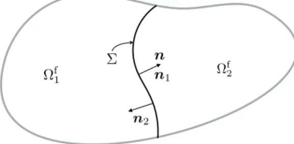
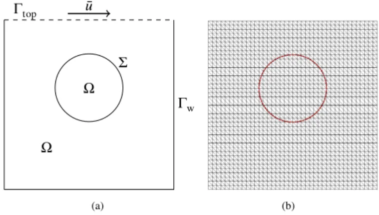
We first consider a linear fluid-structure interaction problem in which the fluid is described by the Stokes equations in a fixed domain and the structure by a linear immersed thin-walled solid model. We denote by Σ ⊂ ℝ𝑑, with 𝑑 = 2, 3, the reference
configuration of the solid mid-surface. The structure is supposed to be immersed within a fixed domain Ω ⊂ ℝ𝑑, with boundary
Γ = 𝜕Ω(see Figure 1). In this section, we assume that the solid undergoes infinitesimal displacements so that the fluid flows within the fixed domain Ωf def= Ω∖Σ ⊂ ℝ𝑑. The immersed interface Σ is supposed to divide Ωfinto two subdomais Ωf = Ωf
1∪Ω f 2,
with respective unit normals 𝒏1 def
= 𝒏Σand 𝒏2def= −𝒏Σ. Here, 𝒏Σthe normal unit vector given by the orientation of the surface Σ. For a given field 𝑓 defined in Ωf (possibly discontinuous across the interface), we can then define its sided-restrictions, denoted
⌦f1
<latexit sha1_base64="1QEPJxTFSinjrFsQ429TQUM1Ee4=">AAAB+XicbVBNS8NAEJ3Ur1q/oh69LBbBU0mqoMeiF29WsB/QxLDZbtqlu0nY3RRK6D/x4kERr/4Tb/4bt20O2vpg4PHeDDPzwpQzpR3n2yqtrW9sbpW3Kzu7e/sH9uFRWyWZJLRFEp7IbogV5SymLc00p91UUixCTjvh6Hbmd8ZUKpbEj3qSUl/gQcwiRrA2UmDb3r2gAxy4T7knBYqmgV11as4caJW4BalCgWZgf3n9hGSCxppwrFTPdVLt51hqRjidVrxM0RSTER7QnqExFlT5+fzyKTozSh9FiTQVazRXf0/kWCg1EaHpFFgP1bI3E//zepmOrv2cxWmmaUwWi6KMI52gWQyozyQlmk8MwUQycysiQywx0SasignBXX55lbTrNfeiVn+4rDZuijjKcAKncA4uXEED7qAJLSAwhmd4hTcrt16sd+tj0Vqyiplj+APr8wf6BJM7</latexit>
⌦<latexit sha1_base64="yLCIlA/nlQ5/LVLMLcraWhAg2dQ=">AAAB+XicbVBNS8NAEJ3Ur1q/oh69LBbBU0mqoMeiF29WsB/QxLDZbtqlu0nY3RRK6D/x4kERr/4Tb/4bt20O2vpg4PHeDDPzwpQzpR3n2yqtrW9sbpW3Kzu7e/sH9uFRWyWZJLRFEp7IbogV5SymLc00p91UUixCTjvh6Hbmd8ZUKpbEj3qSUl/gQcwiRrA2UmDb3r2gAxzUn3JPChRNA7vq1Jw50CpxC1KFAs3A/vL6CckEjTXhWKme66Taz7HUjHA6rXiZoikmIzygPUNjLKjy8/nlU3RmlD6KEmkq1miu/p7IsVBqIkLTKbAeqmVvJv7n9TIdXfs5i9NM05gsFkUZRzpBsxhQn0lKNJ8Ygolk5lZEhlhiok1YFROCu/zyKmnXa+5Frf5wWW3cFHGU4QRO4RxcuIIG3EETWkBgDM/wCm9Wbr1Y79bHorVkFTPH8AfW5w/7kJM8</latexit> f2
by 𝑓1and 𝑓2, as 𝑓1(𝒙)def= lim 𝜉→0−𝑓(𝒙 + 𝜉𝒏1), 𝑓2(𝒙) def = lim 𝜉→0−𝑓(𝒙 + 𝜉𝒏2),
for all 𝒙 ∈ Σ, and the following jump and average operators across Σ:
J𝑓K def = 𝑓1− 𝑓2 J𝑓𝒏K def = 𝑓1𝒏1+ 𝑓2𝒏2, {{𝑓 }}def= 1 2 ( 𝑓1+ 𝑓2).
In this framework, the considered coupled problem reads as follow: find the fluid velocity and pressure 𝒖 ∶ Ω × ℝ+ → ℝ𝑑,
𝑝∶ Ω × ℝ+→ ℝ, the solid displacement and velocity 𝒅 ∶ Σ × ℝ+→ ℝ𝑑,𝒅. ∶ Σ × ℝ+→ ℝ𝑑such that for all 𝑡 ∈ ℝ+we have
⎧ ⎪ ⎨ ⎪ ⎩ 𝜌f𝜕𝑡𝒖− div𝝈(𝒖, 𝑝) = 𝟎 in Ωf, div𝒖 = 0 in Ωf, 𝒖= 𝟎 on Γ, (1) ⎧ ⎪ ⎨ ⎪ ⎩ 𝜌s𝜖𝜕𝑡𝒅. + 𝑳𝒅 = 𝑻 in Σ, . 𝒅= 𝜕𝑡𝒅 in Σ, 𝒅= 𝟎 on 𝜕Σ, (2) { 𝒖=𝒅. on Σ, 𝑻 = −J𝝈(𝒖, 𝑝)𝒏K on Σ (3) with the initial conditions 𝒖(0) = 𝒖0, 𝒅(0) = 𝒅0 and
.
𝒅(0) = 𝒅.0. Here, the symbols 𝜌f and 𝜌sstand respectively the fluid and
solid densities, the thickness of the solid is denoted by 𝜖 and the fluid Cauchy stress tensor is given by
𝝈(𝒖, 𝑝)def= 2𝜇𝝐(𝒖) − 𝑝𝑰 , 𝝐(𝒖)def= 1 2 (
𝛁𝒖+ 𝛁𝒖T),
where 𝜇 denotes the fluid dynamic viscosity. The operator 𝑳 describes the elastic behavior of the solid. The relations in (3) enforce, respectively, the kinematic and dynamic interface coupling conditions. Note that the former enforces two conditions since it has to be seen as 𝒖1= 𝒖2=
.
𝒅on Σ.
2.1
Time-discretization: semi-implicit coupled scheme
In what follows, we will use the following notation for the first-order backward difference: 𝜕𝜏𝑥𝑛
def
= (𝑥𝑛− 𝑥𝑛−1)∕𝜏, where 𝜏 > 0
denotes the time-step length. For the time discretization of the coupled problem (1)-(3) we consider the projection based semi-implicit splitting scheme proposed in27,29for the case of fitted-mesh spatial approximations (see also30,31,32,33). The scheme
avoids strong coupling without compromising stability and accuracy. The fundamental idea consists in combining a fractional-step time-marching in the fluid with a semi-implicit treatment of the interface coupling (3). The resulting time semi-discrete method reads as follows (see27,29) for 𝑛 ≥ 1:
1. Explicit fluid viscous step: Find ̃𝒖𝑛
∶ Ωf → ℝ𝑑such that ⎧ ⎪ ⎪ ⎨ ⎪ ⎪ ⎩ 𝜌f 𝜏(̃𝒖 𝑛 − 𝒖𝑛−1) − div𝝈(̃𝒖𝑛, 𝑝𝑛−1) = 𝟎 in Ωf, ̃ 𝒖𝑛= 𝟎 on Γ, ̃ 𝒖𝑛=𝒅.𝑛−1 on Σ. (4)
2. Implicit pressure-displacement step: Find 𝒖𝑛∶ Ωf → ℝ𝑑, 𝑝𝑛 ∶ Ωf → ℝ, 𝒅𝑛
∶ Σ → ℝ𝑑and𝒅.𝑛 ∶ Σ → ℝ𝑑such that ⎧ ⎪ ⎪ ⎨ ⎪ ⎪ ⎩ 𝜌f 𝜏(𝒖 𝑛 − ̃𝒖𝑛) + 𝛁(𝑝𝑛− 𝑝𝑛−1)= 0 in Ωf, div𝒖𝑛 = 0 in Ωf, 𝒖𝑛⋅ 𝒏 = 0 on Γ, (5) ⎧ ⎪ ⎨ ⎪ ⎩ 𝜌s𝜀𝜕𝜏 . 𝒅𝑛+ 𝑳𝒅𝑛= 𝑻𝑛 on Σ, . 𝒅𝑛= 𝜕𝜏𝒅 𝑛 on Σ, 𝒅𝑛= 𝟎 on 𝜕Σ, (6)
{ 𝒖𝑛𝑖 ⋅ 𝒏𝑖= . 𝒅𝑛⋅ 𝒏𝑖 on Σ, 𝑖 = 1, 2, 𝑻𝑛= −J𝝈(̃𝒖 𝑛 , 𝑝𝑛)𝒏K on Σ. (7)
The viscous-step (4) is loosely coupled with the solid, which avoids strong coupling, whereas the step (5)-(7) guarantees added-mass free stability by the implicit treatment of the fluid pressure and solid inertia. From a computational point of view, the scheme can be reformulated exclusively in terms of ̃𝒖𝑛
, 𝑝𝑛, 𝒅𝑛and𝒅.𝑛as shown in Algorithm 1, where the end-of-step velocity
𝒖𝑛has been eliminated by inserting (5)
1into (4)1and by applying (5)2to (5)1in each sub-domain Ω𝑖. Here, we have used the
notation 𝑝𝑛,⋆def= 2𝑝𝑛−1− 𝑝𝑛−2for the second-order temporal extrapolation of the pressure.
Algorithm 1Time semi-discrete projection based semi-implicit scheme (from27,29).
For 𝑛 ≥ 2:
1. Fluid viscous step: Find ̃𝒖𝑛
∶ Ωf → ℝ𝑑such that ⎧ ⎪ ⎨ ⎪ ⎩ 𝜌f𝜕𝜏̃𝒖𝑛− div𝝈(̃𝒖𝑛, 𝑝𝑛,⋆) = 𝟎 in Ωf, ̃ 𝒖𝑛= 𝟎 on Γ, ̃𝒖𝑛=𝒅.𝑛−1 on Σ. (8)
2. Pressure-displacement step: Find 𝑝𝑛∶ Ωf → ℝ, 𝒅𝑛
∶ Σ → ℝ𝑑and𝒅.𝑛 ∶ Σ → ℝ𝑑such that ⎧ ⎪ ⎨ ⎪ ⎩ −𝜏 𝜌fΔ ( 𝑝𝑛− 𝑝𝑛−1)= −diṽ𝒖𝑛 in Ωf, 𝜏 𝜌f𝛁 ( 𝑝𝑛− 𝑝𝑛−1)⋅ 𝒏 = 0 on Γ, (9) ⎧ ⎪ ⎨ ⎪ ⎩ 𝜌s𝜀𝜕𝜏𝒅.𝑛+ 𝑳𝒅𝑛= 𝑻𝑛 on Σ, . 𝒅𝑛= 𝜕𝜏𝒅 𝑛 on Σ, 𝒅𝑛= 𝟎 on 𝜕Σ, (10) ⎧ ⎪ ⎨ ⎪ ⎩ 𝜏 𝜌f𝛁 ( 𝑝𝑛𝑖 − 𝑝𝑛𝑖−1)⋅ 𝒏𝑖= (̃𝒖 𝑛 −𝒅.𝑛)⋅ 𝒏𝑖 on Σ, 𝑖 = 1, 2, 𝑻𝑛= −J𝝈(̃𝒖 𝑛 , 𝑝𝑛)𝒏K on Σ. (11)
An energy based stability result for the non-incremental version of (4)-(7) (i.e., with 𝑝𝑛−1 = 0) with a fitted mesh based finite
element approximation in space, has been reported in27. Therein, stability is guaranteed under the CFL-like condition
𝜌fℎ2+ 2𝜇𝜏 ≲ 𝜌s𝜀ℎ, (12) where ℎ > 0 stands for the spatial grid parameter. Numerical evidence in27 indicates that (12) is not necessary for stability. It
is also worth noting that unconditional stability was achieved in32 via a specific Nitsche’s treatment of the viscous coupling.
Unfortunately, the splitting error of the resulting scheme is known to be non uniform with respect to ℎ, namely, to scales as (𝜏∕ℎ), so that suitable correction iterations are needed to enhance accuracy under restrictive constraints on the discretization parameters (as in19).
Remark 1. Note that from the relation (11)1we get the continuity of flux on the pressure increment across Σ, namely,
J𝛁
(
𝑝𝑛− 𝑝𝑛−1)⋅ 𝒏K= 0 on Σ.
However, both the pressure 𝑝𝑛and the pressure increment 𝑝𝑛− 𝑝𝑛−1are generally discontinuous across Σ, so that the
pressure-Poisson equation (9)1 is not valid across Σ, only in Ωf. Nevertheless, most of the immersed boundary and fictitious domain
2.2
Unfitted mesh approximation: fully discrete scheme
In the following, the closed spaces 𝐻1
Γ(𝜔), of functions in 𝐻1(𝜔)with zero trace on Γ, and 𝐿20(𝜔), of functions in 𝐿
2(𝜔)with
zero mean in 𝜔, will be considered. The scalar product in 𝐿2(𝜔)is denoted by (⋅, ⋅)
𝜔. In this section we introduce a consistent
unfitted mesh spatial approximation of the time semi-discrete scheme given by Algorithm 1. The fluid fields (̃𝒖𝑛
, 𝑝𝑛)will hence
be approximated in triangulations of Ω which are independent of Σ. To this purpose, it is important to note that: • The velocity gradient 𝛁̃𝒖𝑛
and the pressure 𝑝𝑛are discontinuous across Σ;
• The bulk relations (8)1and (9)1are not valid across Σ, only in Ωf (see Remark 1).
In the case of fitted mesh approximations, these discontinuous features of the solution can be introduced in the discrete approx-imation in simple fashion (e.g., by considering cracked meshes with duplicated nodes on the interface). However, if the fluid mesh does not have a geometrical representation of the interface Σ, guaranteeing consistency of the approximations requires a specific treatment. In this paper, we build on the uniftted Nitsche’s based method for incompressible fluid-structure interaction with overlapping meshes reported in18,19. The fundamental reasons for this choice are: (i) it is Lagrange multipliers free and
ro-bust; (ii) it is mathematically sound (i.e., optimal error estimates are obtained for spatial semi-discrete approximations of linear model problems such as (1)-(3) under reasonable regularity assumptions18); and (iii) it naturally provides a consistent of the
pressure-Poisson problem in step 2 of Algorithm 1.
In order to simplify the presentation, we assume that both Ω and Σ are polyhedral. Let be {s
ℎ}0<ℎ<1a familly of triangulations
of Σ. We then consider the standard space of continuous piecewise affine functions: 𝑋ℎs def= {𝑣ℎ∈ 𝐶0(Σ)/𝑣ℎ|𝐾 ∈ ℙ1(𝐾), ∀𝐾 ∈ℎs
} .
The weak form of the abstract solid elastic operator 𝑳 in (2) is assumed to be given by a positive and symmetric bi-linear form 𝑎s ∶ 𝑾 × 𝑾 ←→ ℝ, where 𝑾 = [𝐻1(Σ)]𝑑
0 denotes the space of admissible displacements. The discrete space for the solid
displacement and velocity approximations is hence defined as 𝑾ℎ = [𝑋ℎs]
𝑑 ∩ 𝑾. For the fluid, we introduce two family of
meshes {ℎ,𝑖}0<ℎ<1, 𝑖 = 1, 2, where each ℎ,𝑖covers the 𝑖-th fluid region Ωf𝑖 defined by Σ. Each mesh ℎ,𝑖is fitted to the exterior
boundary Γ but not to s
ℎ. Furthermore for every element 𝐾 ∈ ℎ,1∩ℎ,2we assume that 𝐾 ∩ Σ𝑛ℎ ≠ ∅. We denote by Ωℎ,𝑖the
⌦ vh,12 Xh,1 <latexit sha1_base64="bvAA2TrDKFQkb4BVVZCEzBAMo40=">AAAB/HicbZDLSsNAFIZPvNZ6i3bpZrAILqQkVdBl0Y3LCvYCbQiT6aQdOpmEmUkhhPoqblwo4tYHcefbOG2z0NYfBj7+cw7nzB8knCntON/W2vrG5tZ2aae8u7d/cGgfHbdVnEpCWyTmsewGWFHOBG1ppjntJpLiKOC0E4zvZvXOhErFYvGos4R6ER4KFjKCtbF8uzLx89GFO+0zgboLRL5ddWrOXGgV3AKqUKjp21/9QUzSiApNOFaq5zqJ9nIsNSOcTsv9VNEEkzEe0p5BgSOqvHx+/BSdGWeAwliaJzSau78nchwplUWB6YywHqnl2sz8r9ZLdXjj5UwkqaaCLBaFKUc6RrMk0IBJSjTPDGAimbkVkRGWmGiTV9mE4C5/eRXa9Zp7Was/XFUbt0UcJTiBUzgHF66hAffQhBYQyOAZXuHNerJerHfrY9G6ZhUzFfgj6/MHUVWT5g==</latexit> v<latexit sha1_base64="JzR65WulX1l1hj86MrCTcSJBdOw=">AAAB+3icbZDLSsNAFIZPvNZ6i3XpZrAILqQkVdBl0Y3LCvYCbQiT6aQdOpmEmUmxhLyKGxeKuPVF3Pk2TtsstPWHgY//nMM58wcJZ0o7zre1tr6xubVd2inv7u0fHNpHlbaKU0loi8Q8lt0AK8qZoC3NNKfdRFIcBZx2gvHdrN6ZUKlYLB71NKFehIeChYxgbSzfrkz8bHRRz/tMoO4Cfbvq1Jy50Cq4BVShUNO3v/qDmKQRFZpwrFTPdRLtZVhqRjjNy/1U0QSTMR7SnkGBI6q8bH57js6MM0BhLM0TGs3d3xMZjpSaRoHpjLAeqeXazPyv1kt1eONlTCSppoIsFoUpRzpGsyDQgElKNJ8awEQycysiIywx0SausgnBXf7yKrTrNfeyVn+4qjZuizhKcAKncA4uXEMD7qEJLSDwBM/wCm9Wbr1Y79bHonXNKmaO4Y+szx/4XZO+</latexit> h,22 Xh,2 Th,2 <latexit sha1_base64="WQXCTAGxL8gp5gxhA2CHyiKBrNg=">AAAB+nicbVDLSsNAFL2pr1pfqS7dBIvgQkpSBV0W3bis0Be0IUymk3boZBJmJkqJ+RQ3LhRx65e482+ctFlo64GBwzn3cs8cP2ZUKtv+Nkpr6xubW+Xtys7u3v6BWT3syigRmHRwxCLR95EkjHLSUVQx0o8FQaHPSM+f3uZ+74EISSPeVrOYuCEacxpQjJSWPLM6DJGaYMTSdualk/NG5pk1u27PYa0SpyA1KNDyzK/hKMJJSLjCDEk5cOxYuSkSimJGssowkSRGeIrGZKApRyGRbjqPnlmnWhlZQST048qaq783UhRKOQt9PZkHlcteLv7nDRIVXLsp5XGiCMeLQ0HCLBVZeQ/WiAqCFZtpgrCgOquFJ0ggrHRbFV2Cs/zlVdJt1J2LeuP+sta8KeoowzGcwBk4cAVNuIMWdADDIzzDK7wZT8aL8W58LEZLRrFzBH9gfP4AOTCT+A==</latexit> Th,1 <latexit sha1_base64="mR5HQ2qFE7FF8uGNI4qc9S/t6Cs=">AAAB+nicbVDLSsNAFL2pr1pfqS7dBIvgQkpSBV0W3bis0Be0IUymk3boZBJmJkqJ+RQ3LhRx65e482+ctFlo64GBwzn3cs8cP2ZUKtv+Nkpr6xubW+Xtys7u3v6BWT3syigRmHRwxCLR95EkjHLSUVQx0o8FQaHPSM+f3uZ+74EISSPeVrOYuCEacxpQjJSWPLM6DJGaYMTSdualk3Mn88yaXbfnsFaJU5AaFGh55tdwFOEkJFxhhqQcOHas3BQJRTEjWWWYSBIjPEVjMtCUo5BIN51Hz6xTrYysIBL6cWXN1d8bKQqlnIW+nsyDymUvF//zBokKrt2U8jhRhOPFoSBhloqsvAdrRAXBis00QVhQndXCEyQQVrqtii7BWf7yKuk26s5FvXF/WWveFHWU4RhO4AwcuIIm3EELOoDhEZ7hFd6MJ+PFeDc+FqMlo9g5gj8wPn8AN6uT9w==</latexit> ⌃<latexit sha1_base64="8uUTfaFO8A7AyjqC00nNqslPKhE=">AAAB7XicdVDLSsNAFJ34rPVVdelmsAiuQpKGtu6KblxWtA9oQ5lMJ+3YmUyYmQgl9B/cuFDErf/jzr9x0lZQ0QMXDufcy733hAmjSjvOh7Wyura+sVnYKm7v7O7tlw4O20qkEpMWFkzIbogUYTQmLU01I91EEsRDRjrh5DL3O/dEKiriWz1NSMDRKKYRxUgbqd2/oSOOBqWyY5/Xq55fhY7tODXXc3Pi1fyKD12j5CiDJZqD0nt/KHDKSawxQ0r1XCfRQYakppiRWbGfKpIgPEEj0jM0RpyoIJtfO4OnRhnCSEhTsYZz9ftEhrhSUx6aTo70WP32cvEvr5fqqB5kNE5STWK8WBSlDGoB89fhkEqCNZsagrCk5laIx0girE1ARRPC16fwf9L2bLdie9d+uXGxjKMAjsEJOAMuqIEGuAJN0AIY3IEH8ASeLWE9Wi/W66J1xVrOHIEfsN4+Acy8j0k=</latexit>
|
{z
}
⌦f 1 <latexit sha1_base64="TdIVAldTj3zR/rc26hwD2dzpuCY=">AAACI3icbVA9T8MwEHXKVylfAUYWiwqJqUoACcRUwcJGkSggNSVynEuxajup7SBVUf4LC3+FhQGEWBj4L7ilA1CedKen9+5k34syzrTxvA+nMjM7N79QXawtLa+srrnrG1c6zRWFNk15qm4iooEzCW3DDIebTAEREYfrqH868q/vQWmWykszzKArSE+yhFFirBS6x0EuY1CRIhSKYDDISTzdMS7DIjgX0CO3RaAETsrQL0O37jW8MfA08SekjiZohe5bEKc0FyAN5UTrju9lplsQZRjlUNaCXENGaJ/0oGOpJAJ0txjfWOIdq8Q4SZUtafBY/blREKH1UER2UhBzp/96I/E/r5Ob5KhbMJnlBiT9fijJOTYpHgWGY6aAGj60hFDF7F8xvSM2L2NjrdkQ/L8nT5OrvYa/39i7OKg3TyZxVNEW2ka7yEeHqInOUAu1EUUP6Am9oFfn0Xl23pz379GKM9nZRL/gfH4BJO6lxQ==</latexit>|
{z
}
⌦f 2 <latexit sha1_base64="RBgbWtCxfEcSx86iG/emL/g4J9I=">AAACHXicbVC7TsMwFHV4lvIKMLJYVEhMVVIqwVjBwkaRaEFqSuQ4N8XCdlLbQaqi/AgLv8LCAEIMLIi/wS0deB3pXh2dc6/se6KMM20878OZmZ2bX1isLFWXV1bX1t2Nza5Oc0WhQ1OeqsuIaOBMQscww+EyU0BExOEiujke+xe3oDRL5bkZZdAXZCBZwigxVgrdZpDLGFSkCIUiGA5zEn/vGJdhEZwKGJCrIlACJ2XYKEO35tW9CfBf4k9JDU3RDt23IE5pLkAayonWPd/LTL8gyjDKoawGuYaM0BsygJ6lkgjQ/WJyXYl3rRLjJFW2pMET9ftGQYTWIxHZSUHMtf7tjcX/vF5uksN+wWSWG5D066Ek59ikeBwVjpkCavjIEkIVs3/F9JrYpIwNtGpD8H+f/Jd0G3V/v944a9ZaR9M4Kmgb7aA95KMD1EInqI06iKI79ICe0LNz7zw6L87r1+iMM93ZQj/gvH8CARqjEg==</latexit>Figure 2One dimensional illustration of the construction of the discrete spaces 𝑋ℎ,𝑖.
domain covered by ℎ,𝑖, viz.,
Ωℎ,𝑖
def
= int(∪𝐾∈ℎ,𝑖𝐾
) .
We shall also make use of the following notation for the broken 𝐿2-product in the whole computational domain
(⋅, ⋅)ℎ def = 2 ∑ 𝑖=1 ∑ 𝐾∈ℎ,𝑖 (⋅, ⋅)𝐾.
For 𝑖 = 1, 2, we can hence introduce the following spaces of continuous piecewise affine functions: 𝑋ℎ,𝑖def= {𝑣ℎ∈ 𝐶0(Ωℎ,𝑖)
/
𝑣ℎ|𝐾 ∈ ℙ1(𝐾), ∀𝐾 ∈ℎ,𝑖
} ,
For the approximation of the fluid velocity and pressure we will consider the following discrete product spaces 𝑽ℎdef= ([𝑋ℎ,1]2× [𝑋 ℎ,2]2 ) ∩ [𝐻1 Γ(Ω)] 𝑑, 𝑄 ℎ def = (𝑋ℎ,1× 𝑋ℎ,2) ∩ 𝐿2(Ω) 0, (13)
which guarantee that interfacial (strong and weak) discontinuities are included in the discrete approximation of both the fluid velocity and pressure. Indeed, the functions of (13) are continuous in the physical fluid domain Ωf but discontinuous across the
interface Σ (see Figure 2). Since the discrete pair 𝑽ℎ∕𝑄ℎis not inf-sup stable, we consider a symmetric stabilization operator,
such as, the one given by Continuous Interior Penalty method (see34) over the whole computational domain:
𝑠ℎ(𝑝ℎ, 𝑞ℎ) = 𝛾pℎ3 𝜇 2 ∑ 𝑖=1 ∑ 𝐹∈ℎ,𝑖 ( J𝛁𝑝ℎK𝐹,J𝛁𝑞ℎK𝐹 ) 𝐹,
where ℎ,𝑖denotes the set of interior edges or faces of ℎ,𝑖. Finally, we introduce the fluid discrete viscous bi-linear form
𝑎fℎ(𝒖ℎ,𝒗ℎ)def= 2𝜇(𝝐(𝒖ℎ), 𝝐(𝒗ℎ)
)
Ωf + 𝑔ℎ(𝒖ℎ,𝒗ℎ),
where the ghost-penalty operator is given by (see35)
𝑔ℎ(𝒖ℎ,𝒗ℎ) def = 𝛾g𝜇ℎ 2 ∑ 𝑖=1 ∑ 𝐹∈Σ 𝑖,ℎ ( J𝛁𝒖𝑖,ℎK𝐹,J𝛁𝒗𝑖,ℎK𝐹 ) 𝐹 (14) and where Σ
𝑖,ℎdenotes the set of interior edges or faces of the elements intersected by Σ. This operator guarantees robustness
irrespectively to the way the interface is cutting the fluid mesh, by extending the coercivity of the viscous bi-linear form to the whole computational domain.
We can now introduce the unfitted mesh approximation of Algorithm 1 detailed in Algorithm 2. Its main ingredients are the following:
• Unfitted Nitsche’s mortaring for the spatial discretization of the the kinematic/dynamic viscous coupling in (8), (10) and (11), which is Lagrange multipliers free (i.e., without additional unknowns) and guarantees accuracy and robustness; • For robustness, the Laplacian operator in the projection-step (9) is integrated over the whole computational domain,
whereas for concistency the remaining fluid bulk terms in (8) and in (9) are integrated in the whole physical domain. Note that the price to pay for consistency in the last point is a specific track of the interface intersections and the integration over cut elements (see, e.g.,36,19and the references therein). As regards the first point, it should be noted that in (16) the discrete
interface stresses are exactly the variationally consistent viscous stress of (8). This constitutes a fundamental difference with respect to the Robin based semi-implicit and explicit coupling schemes respectively reported in32,19with fitted meshes. The
main reason is to avoid the accuracy loss observed with this methods (see Section 2.1). The next section is devoted the energy based stability analysis of Algorithm 2.
Remark 2. In the case in which the interface has a boundary inside the fluid domain (the tip), we consider the construction of the fluid and solid spaces proposed in19, which basically consists in introduce a virtual boundary ̃Σ which closes the fluid domain
(see Figure 3).
⌃
<latexit sha1_base64="xQdIK5uAthh25ryXwEv4E+kZ9Ms=">AAAB73icbVA9T8MwEL2Ur1K+CowsFi0SU5WUAcYKFsYi6IfURpXjOq1V2wm2g1RF/RMsDCDEyt9h49/gphmg5UknPb13p7t7QcyZNq777RTW1jc2t4rbpZ3dvf2D8uFRW0eJIrRFIh6pboA15UzSlmGG026sKBYBp51gcjP3O09UaRbJBzONqS/wSLKQEWys1K3279lI4OqgXHFrbga0SrycVCBHc1D+6g8jkggqDeFY657nxsZPsTKMcDor9RNNY0wmeER7lkosqPbT7N4ZOrPKEIWRsiUNytTfEykWWk9FYDsFNmO97M3F/7xeYsIrP2UyTgyVZLEoTDgyEZo/j4ZMUWL41BJMFLO3IjLGChNjIyrZELzll1dJu17zLmr1u3qlcZ3HUYQTOIVz8OASGnALTWgBAQ7P8ApvzqPz4rw7H4vWgpPPHMMfOJ8/JmOPYQ==</latexit>
e ⌃<latexit sha1_base64="8spl5NvPLQapKesW6MKBuXFuCiI=">AAAB+3icbVBNT8JAEN3iF+JXxaOXjWDiibR40CPRi0eM8pHQhmy3U9iw2za7W5UQ/ooXDxrj1T/izX/jAj0o+JJJXt6bycy8IOVMacf5tgpr6xubW8Xt0s7u3v6BfVhuqySTFFo04YnsBkQBZzG0NNMcuqkEIgIOnWB0PfM7DyAVS+J7PU7BF2QQs4hRoo3Ut8tV75GFoBkPwbtjA0Gqfbvi1Jw58Cpxc1JBOZp9+8sLE5oJiDXlRKme66TanxCpGeUwLXmZgpTQERlAz9CYCFD+ZH77FJ8aJcRRIk3FGs/V3xMTIpQai8B0CqKHatmbif95vUxHl/6ExWmmIaaLRVHGsU7wLAgcMglU87EhhEpmbsV0SCSh2sRVMiG4yy+vkna95p7X6rf1SuMqj6OIjtEJOkMuukANdIOaqIUoekLP6BW9WVPrxXq3PhatBSufOUJ/YH3+AHQLlA0=</latexit>
Figure 3Case in which the Σ has a boundary inside the fluid domain.
Then, we enforce the kinematic/dynamic continuity of the fluid on ̃Σ in a discontinuous Galerkin fashion (see, e.g.,37). More
precisely, the following terms are added −({{𝝈(̃𝒖𝑛ℎ,0)}}𝒏,J̃𝒗ℎK ) ̃ Σ− ( {{𝝈(̃𝒗ℎ,0)}}𝒏,J̃𝒖 𝑛 ℎK ) ̃ Σ+ 𝛾𝜇 ℎ ( J̃𝒖 𝑛 ℎK,J̃𝒗ℎK ) ̃ Σ, ( J𝑝 𝑛,⋆ ℎ K,{{̃𝒗ℎ}}⋅ 𝒏 ) ̃ Σ, (17)
Algorithm 2Projection based semi-implicit scheme with unfitted meshes and static interface.
For 𝑛 ≥ 1:
1. Fluid viscous step: Find ̃𝒖𝑛
ℎ∈ 𝑽ℎsuch that 𝜌f(𝜕𝜏̃𝒖𝑛ℎ, ̃𝒗ℎ) Ωf + 𝑎 f ℎ ( ̃𝒖𝑛ℎ, ̃𝒗ℎ)− 2 ∑ 𝑖=1 ( 𝝈(̃𝒖𝑛ℎ,𝑖,0)𝒏𝑖, ̃𝒗ℎ,𝑖 ) Σ+ 𝛾𝜇 ℎ 2 ∑ 𝑖=1 ( ̃ 𝒖𝑛ℎ,𝑖−𝒅.𝑛ℎ−1, ̃𝒗ℎ,𝑖) Σ − 2 ∑ 𝑖=1 ( ̃ 𝒖𝑛ℎ,𝑖−𝒅.ℎ𝑛−1,𝝈(̃𝒗ℎ,𝑖,0)𝒏𝑖 ) Σ= − ( 𝛁𝑝𝑛,⋆ℎ , ̃𝒗ℎ) Ωf (15) for all ̃𝒗ℎ∈ 𝑽ℎ.
2. Pressure-displacement step: Find(𝑝𝑛 ℎ,𝒅 𝑛 ℎ ) ∈ 𝑄ℎ× 𝑾ℎwith . 𝒅𝑛ℎ= 𝜕𝜏𝒅 𝑛 ℎ, such that ⎧ ⎪ ⎪ ⎨ ⎪ ⎪ ⎩ 𝜏 𝜌f ( 𝛁(𝑝𝑛ℎ− 𝑝𝑛ℎ−1), 𝛁𝑞ℎ ) ℎ+ 𝑠ℎ(𝑝 𝑛 ℎ, 𝑞ℎ) = 2 ∑ 𝑖=1 ( ̃ 𝒖𝑛ℎ,𝑖−𝒅.𝑛ℎ,𝑖, 𝑞ℎ,𝑖𝒏𝑖) Σ− ( div ̃𝒖𝑛ℎ, 𝑞ℎ) Ωf, 𝜌s𝜖(𝜕𝜏𝒅.𝑛ℎ,𝒘ℎ) Σ+ 𝑎 s(𝒅𝑛 ℎ,𝒘ℎ) = 𝛾𝜇 ℎ 2 ∑ 𝑖=1 ( (̃𝒖𝑛ℎ,𝑖−𝒅.𝑛ℎ,𝑖−1), 𝒘ℎ) Σ− 2 ∑ 𝑖=1 ( 𝝈(̃𝒖𝑛ℎ,𝑖, 𝑝𝑛ℎ,𝑖)𝒏𝑖,𝒘ℎ) Σ (16) for all(𝑞ℎ,𝒘ℎ ) ∈ 𝑄ℎ× 𝑾ℎ.
into the left- and right-hand side of step (15), respectively, where as in (16)1we add
−𝜏 𝜌f ( {{𝛁𝑝𝑛ℎ⋅ 𝒏}},J𝑞ℎK ) ̃ Σ− 𝜏 𝜌f ( J𝑝 𝑛 ℎK,{{𝛁𝑞ℎ⋅ 𝒏}} ) ̃ Σ+ 𝜏 𝜌f 𝛾 ℎ ( J𝑝 𝑛 ℎK,J𝑞ℎK ) ̃ Σ, ( J̃𝒖 𝑛 ℎK⋅ 𝒏, {{𝑞ℎ}} ) ̃ Σ, (18)
to the left- and right-hand side, respectively.
2.3
Energy based stability analysis
For the purpose of the analysis below, we recall the following estimate from35:
𝑐g(2𝜇‖𝝐(𝒗ℎ)‖20,Ωℎ+ 𝑔ℎ
(
𝒗ℎ,𝒗ℎ))≤ 2𝜇‖𝝐(𝒗ℎ)‖20,Ωf + 𝑔ℎ
(
𝒗ℎ,𝒗ℎ) (19)
for all 𝒗ℎ∈ 𝑽ℎwith 𝑐g >0and the notation
‖ ⋅ ‖2 0,Ωℎ
def
= (⋅, ⋅)ℎ. We shall also make use of the following (robust) discrete trace inequality
ℎ‖𝝐(𝒗ℎ)𝒏‖20,Σ≤ 𝐶T‖𝝐(𝒗ℎ)‖20,Ωℎ (20)
for all 𝒗ℎ∈ 𝑽ℎ.Let define the discrete total energy 𝐸𝑛ℎby the following expression:
𝐸ℎ𝑛def= 𝜌f 2‖𝒖 𝑛 ℎ‖ 2 0,Ωf + 𝜌s𝜖 2 ‖ . 𝒅𝑛ℎ‖2Σ+ 1 2𝑎 s(𝒅𝑛 ℎ,𝒅 𝑛 ℎ) + 𝜏2 2 𝜌f‖𝛁𝑝 𝑛 ℎ‖ 2 0,Ωℎ.
The following result states the conditional energy based stability of the approximation provided by Algorithm 2.
Theorem 1. Let{(𝒖𝑛ℎ, 𝑝𝑛ℎ,𝒅.𝑛ℎ,𝒅𝑛ℎ)}𝑛
≥1be given by Algorithm 2. Under the following conditions
𝑐g𝛾 ≥ 10𝐶TI,
3𝛾
2𝜇𝜏≤ 𝜌s𝜖ℎ, (21)
the discrete energy estimate presented below holds:
𝐸ℎ𝑛≲ 𝐸0ℎ, (22)
for all 𝑛 ≥ 1. As a result, Algorithm 3 is conditionally stable in the energy norm. Proof. We first introduce the 𝐿2−projection operator 𝜋
ℎ∶ [𝐿2(Ω)]𝑑 → 𝑽ℎgiven by ( 𝜋ℎ𝒔, 𝒗ℎ) Ωf = ( 𝒔, 𝒗ℎ) Ωf (23)
for all 𝒗ℎ ∈ 𝑉 𝑛
ℎ.Note that, depending on how the solid mesh
s
ℎ intersects the fluid overlapping meshes ℎ,𝑖, 𝜋ℎ𝒔may not
be uniquely defined in the whole computation domain. However, a simple argument show that 𝜋ℎ𝒔is uniquely defined in the
physical domain Ωf(it suffices to remove the indetermination by blocking appropirate nodes outside the physical domain). This
feature will be enough for the purpose of the present proof. In a similar fashion, we introduce the intermediate velocity 𝒖𝑛 ℎ∈ 𝑽 𝑛 ℎ given by 𝜌f 𝜏 ( 𝒖𝑛 ℎ,𝒗ℎ ) Ωf = 𝜌f 𝜏 ( ̃ 𝒖𝑛ℎ,𝒗ℎ) Ωf − ( 𝛁(𝑝𝑛 ℎ− 𝑝 𝑛−1 ℎ ), 𝒗ℎ ) Ωf (24) for all 𝒗ℎ∈ 𝑽 𝑛 ℎ, so that 𝒖 𝑛 ℎis uniquely defined in Ω
f. In particular, owing to (23) and (24), we have
𝒖𝑛ℎ= ̃𝒖𝑛ℎ− 𝜏 𝜌f𝜋ℎ𝛁
(
𝑝𝑛ℎ− 𝑝𝑛ℎ−1) in Ωf. (25) Now, since the fluid bulk terms of the viscous step (15) are integrated (only) in the physical domain and using (24), it can alternatively writen as 𝜌f 𝜏 ( ̃𝒖𝑛ℎ, ̃𝒗ℎ) Ω+ 𝑎 f ,𝑛 ℎ ( ̃ 𝒖𝑛ℎ, ̃𝒗ℎ)− 2 ∑ 𝑖=1 ( 𝝈(̃𝒖𝑛ℎ,𝑖,0)𝒏𝑖, ̃𝒗ℎ,𝑖 ) Σ+ 𝛾𝜇 ℎ 2 ∑ 𝑖=1 ( ̃ 𝒖𝑛ℎ,𝑖−𝒅.𝑛ℎ−1, ̃𝒗ℎ,𝑖) Σ − 2 ∑ 𝑖=1 ( ̃ 𝒖𝑛ℎ,𝑖−𝒅.ℎ𝑛−1,𝝈(̃𝒗ℎ,𝑖,0)𝒏𝑖 ) Σ= 𝜌f 𝜏 ( 𝒖𝑛ℎ−1, ̃𝒗ℎ) Ω− ( 𝛁𝑝𝑛ℎ−1, ̃𝒗ℎ) Ω (26) for all ̃𝒗ℎ∈ 𝑽 𝑛 ℎ.
We then proceed by testing the relation (24) with 𝒗𝑛 ℎ= 𝒖 𝑛 ℎ, with yields 𝜌f 2 𝜏[ ‖‖𝒖 𝑛 ℎ‖‖ 2 0,Ωf − ‖‖̃𝒖 𝑛 ℎ‖‖ 2 0,Ωf + ‖‖𝒖 𝑛 ℎ− ̃𝒖 𝑛 ℎ‖‖ 2 0,Ωf ] +(𝛁(𝑝𝑛ℎ− 𝑝ℎ𝑛−1),𝒖𝑛ℎ) Ωf = 0. (27)
By inserting (25) into the last equality and by rearranging the terms we get 𝜌f 2 𝜏[ ‖‖𝒖 𝑛 ℎ‖‖ 2 0,Ωf − ‖‖̃𝒖 𝑛 ℎ‖‖ 2 0,Ωf + ( 𝛁(𝑝𝑛ℎ− 𝑝𝑛ℎ−1), ̃𝒖𝑛ℎ) Ωf − 𝜏 2𝜌f ‖‖‖𝜋ℎ𝛁 ( 𝑝𝑛ℎ− 𝑝𝑛ℎ−1)‖‖‖2 0,Ωf = 0. (28)
On the other hand, by testing (26) with ̃𝒗𝑛 ℎ= ̃𝒖
𝑛
ℎand using (19) we have
𝜌f 2𝜏 [ ‖‖̃𝒖𝑛 ℎ‖‖ 2 0,Ωf − ‖‖‖𝒖 𝑛−1 ℎ ‖‖‖ 2 0,Ωf + ‖‖‖̃𝒖 𝑛 ℎ− 𝒖 𝑛−1 ℎ ‖‖‖ 2 0,Ωf ] + 2𝑐g𝜇 ‖‖𝝐(̃𝒖 𝑛 ℎ)‖‖ 2 0,Ωℎ+ ( 𝛁𝑝𝑛ℎ−1, ̃𝒖𝑛ℎ) Ωf +𝛾 𝜇 ℎ 2 ∑ 𝑖=1 ( ̃𝒖𝑛ℎ,𝑖−𝒅.𝑛ℎ−1, ̃𝒖𝑛ℎ,𝑖) Σ− 2𝜇 2 ∑ 𝑖=1 ( 𝝐(̃𝒖𝑛ℎ,𝑖)𝒏𝑖, ̃𝒖 𝑛 ℎ,𝑖 ) Σ− 2𝜇 2 ∑ 𝑖=1 ( 𝝐(̃𝒖𝑛ℎ,𝑖)𝒏𝑖, ̃𝒖 𝑛 ℎ,𝑖− . 𝒅𝑛ℎ−1) Σ≤ 0 (29)
and by testing the fluid projection-step (16)1with 𝑞ℎ= 𝑝𝑛ℎand by integrating by parts the divergence term we get
𝜏 2 𝜌f[ ‖‖𝛁𝑝 𝑛 ℎ‖‖ 2 0,Ωℎ− ‖‖‖𝛁𝑝 𝑛−1 ℎ ‖‖‖ 2 0,Ωℎ + ‖‖‖𝛁(𝑝𝑛 ℎ− 𝑝 𝑛−1 ℎ )‖‖‖ 2 0,Ωℎ ] −(𝛁𝑝𝑛 ℎ, ̃𝒖 𝑛) Ωf + 2 ∑ 𝑖=1 ( . 𝒅𝑛ℎ,𝒏𝑖𝑝𝑛ℎ,𝑖 ) Σ+ 𝑠ℎ(𝑝 𝑛 ℎ, 𝑝 𝑛 ℎ) = 0. (30)
Finally, by adding the relations (28)-(30) we get the following energy estimate for the fluid 𝜌f 2𝜕𝜏‖‖𝒖 𝑛 ℎ‖‖ 2 0,Ωf + 2𝑐g𝜇 ‖‖𝝐(̃𝒖 𝑛 ℎ)‖‖ 2 0,Ωℎ+ 𝜏 2 𝜌f[ ‖‖𝛁𝑝 𝑛 ℎ‖‖ 2 0,Ωℎ− ‖‖‖𝛁𝑝 𝑛−1 ℎ ‖‖‖ 2 0,Ωℎ ] + 𝜏 2 𝜌f ‖‖‖ ( − 𝜋ℎ ) 𝛁(𝑝𝑛ℎ− 𝑝𝑛ℎ−1)‖‖‖2 Ωf + 𝜏 2 𝜌f ‖‖‖𝛁(𝑝 𝑛 ℎ− 𝑝 𝑛−1 ℎ )‖‖‖ 2 Ωℎ∖Ωf + 2 ∑ 𝑖=1 ( . 𝒅𝑛ℎ,𝒏𝑖𝑝𝑛ℎ,𝑖) Σ + 𝛾 𝜇 ℎ 2 ∑ 𝑖=1 ( ̃ 𝒖𝑛ℎ,𝑖−𝒅.𝑛ℎ−1, ̃𝒖𝑛ℎ,𝑖) Σ− 2𝜇 2 ∑ 𝑖=1 ( 𝝐(̃𝒖𝑛ℎ,𝑖)𝒏𝑖, ̃𝒖 𝑛 ℎ,𝑖 ) Σ− 2𝜇 2 ∑ 𝑖=1 ( 𝝐(̃𝒖𝑛ℎ,𝑖)𝒏𝑖, ̃𝒖 𝑛 ℎ,𝑖− . 𝒅𝑛ℎ−1) Σ≤ 0. (31)
We now proceed by testing the solid equation (16)2with 𝒘ℎ= . 𝒅𝑛ℎ, which yields 𝜌s𝜖 2 𝜏 [ ‖ ‖‖𝒅.𝑛ℎ‖‖ ‖ 2 0,Σ− ‖‖‖ . 𝒅𝑛ℎ−1‖‖ ‖ 2 0,Σ+ ‖‖‖ . 𝒅𝑛ℎ−𝒅.𝑛ℎ−1‖‖ ‖ 2 0,Σ ] + 1 2 𝜏 [ 𝑎s(𝒅𝑛ℎ,𝒅ℎ𝑛) − 𝑎s(𝒅𝑛ℎ−1,𝒅ℎ𝑛−1) + 𝑎s(𝒅𝑛ℎ− 𝒅ℎ𝑛−1,𝒅𝑛ℎ− 𝒅𝑛ℎ−1)] + 2𝜇 2 ∑ 𝑖=1 ( 𝝐(̃𝒖𝑛ℎ,𝑖)𝒏,𝒅.𝑛ℎ) Σ− 2 ∑ 𝑖=1 ( 𝑝𝑛ℎ,𝑖𝒏𝑖,𝒅.𝑛ℎ) Σ− 𝛾 𝜇 ℎ 2 ∑ 𝑖=1 ( ̃ 𝒖𝑛ℎ,𝑖−𝒅.𝑛ℎ−1,𝒅.𝑛ℎ) Σ= 0.
By adding this relation to (31) we get the following total energy estimate 𝜌f 2𝜕𝜏‖‖𝒖 𝑛 ℎ‖‖ 2 0,Ωf + 2𝑐g𝜇 ‖‖𝝐(̃𝒖 𝑛 ℎ)‖‖ 2 0,Ωℎ+ 𝜏 2 𝜌f [ ‖‖𝛁𝑝𝑛 ℎ‖‖ 2 0,Ωℎ− ‖‖‖𝛁𝑝 𝑛−1 ℎ ‖‖‖ 2 0,Ωℎ ] 𝜌s𝜖 2 𝜏 [ ‖ ‖‖𝒅.𝑛ℎ‖‖ ‖ 2 0,Σ− ‖‖‖ . 𝒅𝑛ℎ−1‖‖ ‖ 2 0,Σ+ ‖‖‖ . 𝒅𝑛ℎ−𝒅.𝑛ℎ−1‖‖ ‖ 2 0,Σ ] + 1 2 𝜏 [ 𝑎s(𝒅𝑛ℎ,𝒅𝑛ℎ) − 𝑎s(𝒅𝑛ℎ−1,𝒅𝑛ℎ−1)] −2𝜇 2 ∑ 𝑖=1 ( 𝝐(̃𝒖𝑛ℎ,𝑖)𝒏𝑖, ̃𝒖𝑛ℎ,𝑖−𝒅.𝑛ℎ) Σ− 2𝜇 2 ∑ 𝑖=1 ( 𝝐(̃𝒖𝑛ℎ,𝑖)𝒏𝑖, ̃𝒖𝑛ℎ,𝑖−𝒅.𝑛ℎ−1) Σ ⏟⏞⏞⏞⏞⏞⏞⏞⏞⏞⏞⏞⏞⏞⏞⏞⏞⏞⏞⏞⏞⏞⏞⏞⏞⏞⏞⏞⏞⏞⏞⏞⏞⏞⏞⏞⏞⏞⏞⏞⏞⏞⏞⏞⏞⏞⏞⏞⏞⏞⏞⏞⏟⏞⏞⏞⏞⏞⏞⏞⏞⏞⏞⏞⏞⏞⏞⏞⏞⏞⏞⏞⏞⏞⏞⏞⏞⏞⏞⏞⏞⏞⏞⏞⏞⏞⏞⏞⏞⏞⏞⏞⏞⏞⏞⏞⏞⏞⏞⏞⏞⏞⏞⏞⏟ 𝑇1 +𝛾 𝜇 ℎ 2 ∑ 𝑖=1 ( ̃𝒖𝑛ℎ,𝑖−𝒅.𝑛ℎ−1, ̃𝒖𝑛ℎ,𝑖−𝒅.𝑛ℎ) Σ ⏟⏞⏞⏞⏞⏞⏞⏞⏞⏞⏞⏞⏞⏞⏞⏞⏞⏞⏞⏞⏞⏞⏞⏟⏞⏞⏞⏞⏞⏞⏞⏞⏞⏞⏞⏞⏞⏞⏞⏞⏞⏞⏞⏞⏞⏞⏟ 𝑇2 ≤ 0. (32)
Terms 𝑇1can be bounded from every side of the interface by adding and subtracting
.
𝒅𝑛ℎ, using the Cauchy−Schwarz, Young’s
and trace inequalities (20), as follows:
𝑇1 = −2𝜇(𝝐(̃𝒖𝑛ℎ,𝑖)𝒏𝑖, . 𝒅𝑛ℎ−𝒅.𝑛ℎ−1) Σ− 4𝜇 ( 𝝐(̃𝒖𝑛ℎ,𝑖)𝒏𝑖, ̃𝒖 𝑛 ℎ,𝑖− . 𝒅𝑛ℎ) Σ ≥ −20 𝜇 𝐶TI 𝛾 ‖‖𝝐(̃𝒖 𝑛 ℎ)‖‖ 2 0,Ωℎ− 𝛾 𝜇 4 ℎ‖‖‖̃𝒖 𝑛 ℎ,𝑖− . 𝒅𝑛ℎ‖‖ ‖ 2 0,Σ− 𝛾 𝜇 4 ℎ‖‖‖ . 𝒅𝑛ℎ−𝒅.𝑛ℎ−1‖‖ ‖ 2 0,Σ. (33)
Similarly, for the second term we have 𝑇2= 𝛾 𝜇 ℎ ‖‖‖̃𝒖 𝑛 ℎ,𝑖− . 𝒅𝑛ℎ‖‖ ‖ 2 0,Σ+ 𝛾 𝜇 ℎ ( . 𝒅𝑛ℎ−𝒅.𝑛ℎ−1, ̃𝒖𝑛ℎ,𝑖−𝒅.𝑛ℎ) Σ ≥ 𝛾 𝜇 2ℎ ‖‖‖̃𝒖 𝑛 ℎ,𝑖− . 𝒅𝑛ℎ‖‖ ‖ 2 0,Σ− 𝛾 𝜇 2 ℎ‖‖‖ . 𝒅𝑛ℎ−𝒅.𝑛ℎ−1‖‖ ‖ 2 0,Σ. (34) By applying (33)-(34) we get 𝜌f 2𝜕𝜏‖‖𝒖 𝑛 ℎ‖‖ 2 0,Ωf + 2𝜇 ( 𝑐g− 10 𝐶TI 𝛾 ) ‖‖𝝐(̃𝒖𝑛 ℎ)‖‖ 2 0,Ωℎ+ 𝜏 2 𝜌f[ ‖‖𝛁𝑝 𝑛 ℎ‖‖ 2 0,Ωℎ− ‖‖‖𝛁𝑝 𝑛−1 ℎ ‖‖‖ 2 0,Ωℎ ] +𝜌s𝜖 2 𝜕𝜏‖‖‖ . 𝒅𝑛ℎ‖‖ ‖ 2 0,Σ+ (𝜌 s𝜖 2 𝜏 − 3𝛾 𝜇 4 ℎ ) ‖‖ ‖ . 𝒅𝑛ℎ−𝒅.𝑛ℎ−1‖‖ ‖ 2 0,Σ+ 1 2 𝜏 [ 𝑎s(𝒅𝑛ℎ,𝒅ℎ𝑛) − 𝑎s(𝒅𝑛ℎ−1,𝒅 𝑛−1 ℎ ) ] +𝛾 𝜇 4ℎ ‖‖‖̃𝒖 𝑛 ℎ,𝑖− . 𝒅𝑛ℎ‖‖ ‖ 2 0,Σ≤ 0. (35)
Finally, the energy estimate (22) follows from (35) under de assumption (21), which completes the proof.
It is worth noting that the stability condition (21) provided by Theorem 1 is similar to the stability condition (12) obtained in27for Algorithm 1 with fitted meshes.
3
NON-LINEAR MODEL: MOVING INTERFACE
In this section, we propose an extension of the semi-implicit coupling scheme given by Algorithm 2 to the case of non-linear fluid−structure interaction problems involving an incompressible viscous fluid and a moving immersed thin-walled structure. The fluid is described by the Navier-Stokes equations (in Eulerian form) and the structure by a possibly non-linear (beam or shell) solid model (in Lagrangian form).
3.1
Problem setting
Let Ω ⊂ ℝ𝑑 be the reference configuration of the fluid domain with boundary Γ def= 𝜕Ω, and Σ ⊂ ℝ2 be the reference solid
mid-surface. In contrast to Section 2, the structure is now supposed to move within the fluid domain. The current position of the interface Σ(𝑡) is described in terms of a deformation map 𝝓 ∶ Σ × ℝ+ ←→ ℝ𝑑 as Σ(𝑡) = 𝝓(Σ, 𝑡), with 𝝓def= 𝑰
Σ+ 𝒅and where
𝒅denotes the solid displacement. To simplify the notation we will refer to 𝝓𝑡 def= 𝝓(⋅, 𝑡), so that we also have Σ(𝑡) = 𝝓𝑡(Σ).
Note that the fluid control volume is now time-dependent, namely Ωf(𝑡)def= Ω∖Σ(𝑡) ⊂ ℝ𝑑 with boundary 𝜕Ω(𝑡) = Σ(𝑡) ∪ Γ.
The notations introduced in Section 2 for the surface normal vector 𝒏Σ, jumps and average operators remain valid with the sole
difference that they refer to the current interface position Σ(𝑡). The considered coupled problem reads therefore as follow: find the fluid velocity and pressure 𝒖 ∶ Ω × ℝ+ → ℝ𝑑, 𝑝 ∶ Ω × ℝ+ → ℝ, the solid displacement and velocity 𝒅 ∶ Σ × ℝ+ → ℝ𝑑,
.
⎧ ⎪ ⎨ ⎪ ⎩ 𝜌f(𝜕𝑡𝒖+ 𝒖⋅ ∇𝒖)− div𝝈(𝒖, 𝑝) = 𝟎 in Ωf(𝑡), div𝒖 = 0 in Ωf(𝑡), 𝒖= 𝟎 on Γ, (36) ⎧ ⎪ ⎨ ⎪ ⎩ 𝜌s𝜖s𝜕𝑡 . 𝒅+ 𝑳𝒅 = 𝑻 on Σ, . 𝒅= 𝜕𝑡𝒅 on Σ, 𝒅= 𝟎 on 𝜕Σ, (37) ⎧ ⎪ ⎪ ⎨ ⎪ ⎪ ⎩ 𝝓= 𝑰Σ+ 𝒅, Σ(𝑡) = 𝝓𝑡(Σ), Ωf(𝑡) = Ω∖Σ(𝑡), 𝒖=𝒅.◦𝝓−1𝑡 on Σ(𝑡), ∫ Σ 𝑻⋅ 𝒘 = − ∫ Σ(𝑡) J𝝈(𝒖, 𝑝)𝒏K⋅ 𝒘◦𝝓 −1 𝑡 . (38)
The relations in (38) respectively enforce the geometrical compatibility, the kinematic and the dynamic coupling at the interface between the fluid and the solid. In the next section, we propose a numerical method for the coupled system (36)-(38) based on Algorithm 2.
3.2
Numerical methods
With the purpose of avoiding geometrical non-linearities in the fluid, we will discretize the geometric compatibility condition (38)1, namely Ωf(𝑡) = Ω∖Σ(𝑡), in an explicit fashion. For a given displacement approximation 𝒅
𝑛
ℎ ∈ 𝑾ℎ, we define by 𝝓 𝑛 ℎits
associated deformation map as 𝝓𝑛 ℎ
def
= 𝑰Σ+ 𝒅𝑛ℎ. This map characterizes the interface position, at time level 𝑛, as Σ 𝑛 def= 𝝓𝑛
ℎ(Σ).
We hence propose to explicitly update the physical fluid domain as
Ωf ,𝑛 def= Ω∖Σ𝑛−1. (39)
For the fluid discrete spaces, 𝑽𝑛 ℎand 𝑄
𝑛
ℎ, we proceed as in Section 2.2, with the difference that they are now given in term of the
time-dependent overlapping meshes 𝑛
ℎ,𝑖covering each side of Ω
f ,𝑛. We recall that this functional spaces are made of functions
that are continuous in each side of Ωf ,𝑛but discontinuous across Σ𝑛−1. Finally, we introduce the broken 𝐿2-product in the moving
computational domain as (⋅, ⋅)𝑛,ℎ def = 2 ∑ 𝑖=1 ∑ 𝐾∈𝑛 ℎ,𝑖 (⋅, ⋅)𝐾.
The approximation space for the solid 𝑾ℎis the same as in Section 2.2.
For the spatial approximation of the fluid, we introduce the following discrete tri-linear form associated to the convective term 𝑐𝑛(𝒛ℎ,𝒖ℎ,𝒗ℎ) def = 𝜌f(𝒛ℎ⋅ 𝛁𝒖ℎ,𝒗ℎ ) Ωf ,𝑛+ 𝜌f 2 ( (div𝒛ℎ)𝒖ℎ,𝒗ℎ ) Ωf ,𝑛− 𝜌 f({{𝒛 ℎ}}⋅ 𝒏J𝒖ℎK,{{𝒗ℎ}} ) Σ𝑛−1− 𝜌f 2 ( J𝒛ℎ⋅ 𝒏K,{{𝒖ℎ⋅ 𝒗ℎ}} ) Σ𝑛−1, (40)
where the three last terms are added in order to guarantee that 𝑐𝑛(𝒗
ℎ,𝒛ℎ,𝒛ℎ) = 0for all 𝒛ℎ∈ 𝑽 𝑛
ℎ(see19). Numerical instabilities
due to the lack of inf−sup compatibility of the discrete spaces and to large local Reynolds number, will be handled by the continuous interior penalty stabilization method (CIP) of38,39. The associated symmetric velocity and pressure stabilization
operators are given by:
𝑠𝑛v,ℎ(𝒛ℎ; 𝒖ℎ,𝒗ℎ) def = 𝛾vℎ2 2 ∑ 𝑖=1 ∑ 𝐹∈𝑛 ℎ,𝑖 𝜉(Re𝐹(𝒛ℎ) ) ‖𝒛ℎ⋅ 𝒏‖𝐿∞(𝐹 ) ( J𝛁𝒖ℎK𝐹,J𝛁𝒗ℎK𝐹 ) 𝐹, 𝑠𝑛p,ℎ(𝒛ℎ; 𝑝ℎ, 𝑞ℎ) def = 𝛾pℎ2 2 ∑ 𝑖=1 ∑ 𝐹∈𝑛 ℎ,𝑖 𝜉(Re𝐹(𝒛ℎ) ) ‖𝒛ℎ‖𝐿∞(𝐹 ) ( J𝛁𝑝ℎK𝐹,J𝛁𝑞ℎK𝐹 ) 𝐹, where 𝑛
ℎ,𝑖denotes the set of interior edges or faces of 𝑛
ℎ,𝑖, Re𝐹(𝒛ℎ)
def
= 𝜌f‖𝒛
ℎ‖𝐿∞(𝐹 )ℎ𝜇−1 denotes the local Reynolds number,
to the way the interface Σ𝑛is cutting the fluid domain Ω, we introduce the time-dependent ghost-penalty operator, given by 𝑔ℎ𝑛(𝒖ℎ,𝒗ℎ) def = 𝛾g𝜇ℎ 2 ∑ 𝑖=1 ∑ 𝐹∈Σ𝑛−1 𝑖,ℎ ( J𝛁𝒖𝑖,ℎK𝐹,J𝛁𝒗𝑖,ℎK𝐹 ) 𝐹, where Σ𝑛−1
𝑖,ℎ denotes the set of interior edges or faces of the elements intersected by Σ
𝑛−1. Finally, we collect all the above terms
in a single contribution 𝑎f ,𝑛ℎ (𝒛ℎ; 𝒖ℎ,𝒗ℎ )def = 𝑐𝑛(𝒛 ℎ,𝒖ℎ,𝒗ℎ) + 2𝜇 ( 𝝐(𝒖ℎ), 𝝐(𝒗ℎ) ) Ωf ,𝑛+ 𝑠 𝑛 v,ℎ(𝒛ℎ; 𝒖ℎ,𝒗ℎ) + 𝑔𝑛ℎ(𝒖ℎ,𝒗ℎ). (41)
With all the above ingredients, we propose to approximate (36)-(38) by the semi-implicit coupling scheme reported in Algorithm 3. The basic idea consists in combining the interface kinematic/dynamic coupling of Algorithm 2 with the explicit treatment of the geometrical compatibility (39).
Algorithm 3Projection based semi-implicit scheme with unfitted meshes and moving interfaces.
For 𝑛 ≥ 1:
1. Interface update:
Σ𝑛−1 = 𝝓𝑛ℎ−1(Σ), Ωf ,𝑛 = Ω∖Σ𝑛−1. 2. Fluid viscous step: Find ̃𝒖𝑛
ℎ∈ 𝑽 𝑛 ℎsuch that 𝜌f(𝜕𝜏̃𝒖 𝑛 ℎ, ̃𝒗ℎ ) Ωf ,𝑛+ 𝑎 f ,𝑛 ℎ ( ̃𝒖𝑛ℎ−1; ̃𝒖𝑛ℎ, ̃𝒗ℎ)− 2 ∑ 𝑖=1 ( 𝝈(̃𝒖𝑛ℎ,𝑖,0)𝒏𝑖, ̃𝒗ℎ,𝑖 ) Σ𝑛−1+ 𝛾𝜇 ℎ 2 ∑ 𝑖=1 ( ̃ 𝒖𝑛ℎ,𝑖−𝒅.𝑛ℎ−1, ̃𝒗ℎ,𝑖) Σ𝑛−1 − 2 ∑ 𝑖=1 ( ̃ 𝒖𝑛ℎ,𝑖−𝒅.ℎ𝑛−1,𝝈(̃𝒗ℎ,𝑖,0)𝒏𝑖 ) Σ𝑛−1 = − ( 𝛁𝑝𝑛,⋆ℎ , ̃𝒗ℎ) Ωf ,𝑛 (42) for all ̃𝒗ℎ∈ 𝑽 𝑛 ℎ.
3. Pressure-displacement step: Find(𝑝𝑛ℎ,𝒅𝑛ℎ)∈ 𝑄𝑛ℎ× 𝑾ℎwith . 𝒅𝑛ℎ= 𝜕𝜏𝒅 𝑛 ℎ, such that ⎧ ⎪ ⎪ ⎨ ⎪ ⎪ ⎩ 𝜏 𝜌f ( 𝛁(𝑝𝑛 ℎ− 𝑝 𝑛−1 ℎ ), 𝛁𝑞ℎ ) 𝑛,ℎ+ 𝑠 𝑛 p,ℎ(̃𝒖 𝑛 ℎ; 𝑝 𝑛 ℎ, 𝑞ℎ) = 2 ∑ 𝑖=1 ( ̃ 𝒖𝑛ℎ,𝑖−𝒅.𝑛ℎ,𝑖, 𝑞ℎ,𝑖𝒏𝑖) Σ𝑛−1− ( div ̃𝒖𝑛ℎ, 𝑞ℎ) Ωf ,𝑛, 𝜌s𝜖(𝜕𝜏 . 𝒅𝑛ℎ,𝒘ℎ) Σ+ 𝑎 s(𝒅𝑛 ℎ,𝒘ℎ) = 𝛾𝜇 ℎ 2 ∑ 𝑖=1 ( (̃𝒖𝑛ℎ,𝑖−𝒅.𝑛ℎ,𝑖−1), 𝒘ℎ ) Σ𝑛−1− 2 ∑ 𝑖=1 ( 𝝈(̃𝒖𝑛ℎ,𝑖, 𝑝𝑛ℎ,𝑖)𝒏𝑖,𝒘ℎ ) Σ𝑛−1 (43) for all(𝑞ℎ,𝒘ℎ)∈ 𝑄𝑛 ℎ× 𝑾ℎ. Then, set 𝝓 𝑛 ℎ= 𝑰Σ+ 𝒅 𝑛 ℎ.
Note that steps (42) and (43) of Algorithm 3 involves integrals of functions associated with different time levels, namely, ( ̃ 𝒖𝑛ℎ−1, ̃𝒗ℎ) Ω𝑛, ( 𝛁𝑝𝑛ℎ−1, ̃𝒗ℎ) Ω𝑛, ( 𝛁𝑝𝑛ℎ−2, ̃𝒗ℎ) Ω𝑛, ( 𝛁𝑝𝑛ℎ−1,𝛁𝑞ℎ)𝑛,ℎ. with ̃𝒖𝑛 ℎ∈ 𝑽 𝑛 ℎ, 𝑝 𝑛−1 ℎ ∈ 𝑄 𝑛−1 ℎ and 𝑝 𝑛−2 ℎ ∈ 𝑄 𝑛−2
ℎ . This requires the integration of products of functions that might be discontinuous
at different locations in the same element. In order avoid the simultaneous intersection of different interface locations with the same fluid element, we consider the approach introduced in19 (see also40), which basically consists in locally shifting the
discontinuity at time 𝑡⋆to the structure location at time 𝑡𝑛, where 𝑡⋆ refers to 𝑡𝑛−1 and 𝑡𝑛−2respectively. In the case where the
discontinuities are located in different elements, the quadrature is performed in a standard fashion since we keep track of the (previous) intersections at different times and we can treat each discontinuity separately.
Remark 3. In the case of partially intersected fluid domain with dynamic interface, we proceed as in Remark 2. The terms in (17) and (18) are now evaluated on ̃Σ𝑛−1and we add the following convective Discontinuous Galerkin contributions (see, e.g.,37)
to the tri-linear form (40):
−𝜌f({{𝒛ℎ}}⋅ 𝒏J𝒖ℎK,{{𝒗ℎ}} ) ̃ Σ𝑛−1− 𝜌f 2 ( J𝒛ℎ⋅ 𝒏K,{{𝒖ℎ⋅ 𝒗ℎ}} ) ̃ Σ𝑛−1.
Remark 4. Note that whenever𝒅.𝑛ℎ,𝑖,𝒅.ℎ,𝑖𝑛−1and 𝒘ℎare integrated on Σ𝑛−1, one has to understand𝒅.𝑛 ℎ,𝑖◦ ( 𝜙𝑛−1 ℎ )−1 ,𝒅.𝑛ℎ,𝑖−1◦(𝜙𝑛−1 ℎ )−1 and 𝒘ℎ◦ ( 𝜙𝑛−1 ℎ )−1
respectively. This abuse of notation is simply made to ease the presentation.
4
NUMERICAL EXPERIMENTS
In this section we illustrate the stability and accuracy of the proposed semi-implicit scheme (Algorithm 3) in different 2D test cases motivated by the simulation of heart valves and of micro-encapsulation. To this purpose we compare the results obtained with Algorithm 3 and those obtained with the strongly coupled and loosely coupled (stabilized explicit coupling) schemes proposed in19. The implicit step in Algorithm 3 is solved in a partitioned fashion by a Dirichlet-Neumann based Newton-GMRES
iterative algorithm. In all the tests, the solid is described by a non-linear Reissner−Mindlin curved beam model with a MITC spacial discretization. All the units are given in the CGS units system
4.1
Idealized valve without contact
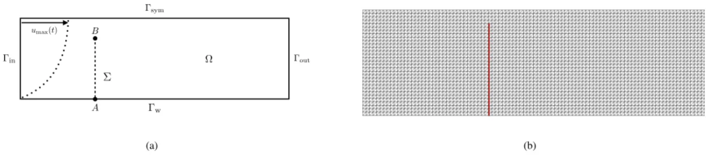
The first example is the heart-valve-inspired benchmark proposed in41,42,43,44,21. The considered geometry is shown in Figure
4(a) . The fluid domain is a rectangle Ω = [0, 8] × [0, 0.805], while the immersed solid reference configuration Σ is the straight segment 𝐴𝐵, with 𝐴 = (2, 0) and 𝐵 = (2, 0.7).
⌦ ⌃ A B sym w out in umax(t) (a) (b)
Figure 4(a) Geometric configuration of the idealized valve without contact, (b) Zoom of the fluid and solid meshes.
The physical parameters used for the fluid in this test are 𝜌f = 100, 𝜇 = 10. While for the solid we have 𝜌s= 100, 𝜖s= 0.0212,
the Young’s modulus 𝐸 = 5.6⋅107and Poisson’s ratio 𝜈 = 0.4. Concerning the boundary conditions, no-slip boundary condition
is apply on Γw, a symmetry condition is imposed on Γsym, zero traction on Γout and finally on Γinthe following half parabolic
profile is applied:
𝑢max(𝑡) = 5(0.805)2(sin(2𝜋𝑡) + 1.1), 𝑡∈ ℝ+.
The solid rotation and displacement are set to zero at the bottom endpoint 𝐴 and rest initial conditions are considered for both fluid and solid.
The solid mesh is made of 64 edges while the fluid unfitted mesh is made of 18662 triangles (see Figure 4(b)). The Nitsche parameter is set to 𝛾 = 10 and the Ghost penalty parameter to 𝛾g = 1. The CIP stabilization parameters are 𝛾v= 𝛾p= 10−2. Three
different levels of time-step refinement, 𝜏 ∈ {(10−3∕2𝑖)}2
𝑖=0, are considered in order to compare results from Algorithms 3 and
the loosely coupled and strongly coupled schemes. The final time is 𝑇 = 3, which corresponds to 3 full oscillations cycles for the structure.
For illustration purposes, snapshots of the fluid velocity magnitude and the position of the interface, computed with 𝜏 = 10−3,
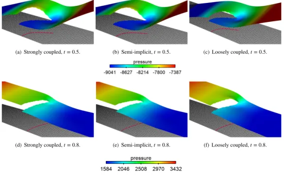
are shown in Figure 5 at time 𝑡 = 0.5 and 𝑡 = 0.8 respectively. A very good agreement is obtained for the three methods already with the larger time step and all algorithms reproduce very well the vortex induced after the leaflet. The two times selected correspond to a situation of opening of the valve at 𝑡 = 0.5 and closing at 𝑡 = 0.8. At opening state, there is an increasing velocity magnitude on top of the channel, while the velocity is decreasing at closing state. Figure 6 presents the pressure elevation computed with the coarsest time step, 𝜏 = 10−3, obtained with the semi-implicit coupling scheme (Algorithm 3), the loosely
(a) Strongly coupled, 𝑡 = 0.5. (b) Semi-implicit, 𝑡 = 0.5. (c) Loosely coupled, 𝑡 = 0.5.
(d) Strongly coupled, 𝑡 = 0.8. (e) Semi-implicit, 𝑡 = 0.8. (f) Loosely coupled, 𝑡 = 0.8.
Figure 5Velocity magnitude snapshots at 𝜏 = 10−3.
(a) Strongly coupled, 𝑡 = 0.5. (b) Semi-implicit, 𝑡 = 0.5. (c) Loosely coupled, 𝑡 = 0.5.
(d) Strongly coupled, 𝑡 = 0.8. (e) Semi-implicit, 𝑡 = 0.8. (f) Loosely coupled, 𝑡 = 0.8.
Figure 6Pressure snapshots at 𝜏 = 10−3.
coupled and the strongly coupled schemes at the same time instants as before. The discontinuity of the pressure is well captured with all methods. A very good agreement can be observed between Algorithm 3 and the strongly coupled scheme, while some differences are clear visible in the loosely coupled scheme.
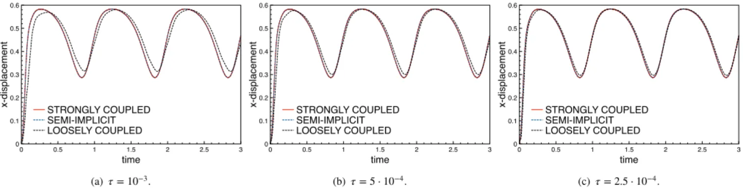
Figures 7 and 8 report the displacement history of the upper structure endpoint 𝐵 as function of time, in terms of 𝑥-displacement and 𝑦-𝑥-displacement respectively. Algorithm 3 delivers practically the same results as the strongly coupled scheme (the two curves are indistinguishable already with the larger time step), whereas some differences are clearly visible with the loosely coupled scheme. This mismatch is reduced with the time-step refinement.