HAL Id: hal-02491495
https://hal.inria.fr/hal-02491495
Submitted on 26 Feb 2020
HAL is a multi-disciplinary open access
archive for the deposit and dissemination of
sci-entific research documents, whether they are
pub-lished or not. The documents may come from
teaching and research institutions in France or
abroad, or from public or private research centers.
L’archive ouverte pluridisciplinaire HAL, est
destinée au dépôt et à la diffusion de documents
scientifiques de niveau recherche, publiés ou non,
émanant des établissements d’enseignement et de
recherche français ou étrangers, des laboratoires
publics ou privés.
between data locality and load balancing
Changjiang Gou, Ali Al Zoobi, Anne Benoit, Mathieu Faverge, Loris Marchal,
Grégoire Pichon, Pierre Ramet
To cite this version:
Changjiang Gou, Ali Al Zoobi, Anne Benoit, Mathieu Faverge, Loris Marchal, et al.. Improving
mapping for sparse direct solvers: A trade-off between data locality and load balancing. [Research
Report] RR-9328, Inria Rhône-Alpes. 2020, pp.21. �hal-02491495�
0249-6399 ISRN INRIA/RR--9328--FR+ENG
RESEARCH
REPORT
N° 9328
February 2020sparse direct solvers:
A trade-off between data
locality and load
balancing
Changjiang Gou, Ali Al Zoobi, Anne Benoit, Mathieu Faverge, Loris
Marchal, Grégoire Pichon, Pierre Ramet
RESEARCH CENTRE GRENOBLE – RHÔNE-ALPES
Inovallée
655 avenue de l’Europe Montbonnot
balancing
Changjiang Gou, Ali Al Zoobi, Anne Benoit, Mathieu Faverge,
Loris Marchal, Gr´
egoire Pichon, Pierre Ramet
Project-Team ROMA
Research Report n° 9328 — February 2020 — 21 pages
Abstract: In order to express parallelism, parallel sparse direct solvers take advantage of the elimination tree to exhibit tree-shaped task graphs, where nodes represent computational tasks and edges represent data dependencies. One of the pre-processing stages of sparse direct solvers consists of mapping computational resources (processors) to these tasks. The objective is to minimize the factorization time by exhibiting good data locality and load balancing. The proportional mapping technique is a widely used approach to solve this resource-allocation problem. It achieves good data locality by assigning the same processors to large parts of the elimination tree. However, it may limit load balancing in some cases. In this paper, we propose a dynamic mapping algorithm based on proportional mapping. This new approach, named Steal, relaxes the data locality criterion to improve load balancing. In order to validate the newly introduced method, we perform extensive experiments on the PaStiX sparse direct solver. It demonstrates that our algorithm enables better static scheduling of the numerical factorization while keeping good data locality.
R´esum´e : Les solveurs parall`eles directs creux se servent de l’arbre d’´elimination pour obtenir des graphes de tˆaches sous forme d’arbres, o`u les nœuds repr´esentent des tˆaches de calcul, et les arˆetes des d´ependances de donn´ees. Une des premi`eres ´
etapes de ces solveurs consiste `a placer les tˆaches sur les ressources (les pro-cesseurs). Le but est de minimiser le temps de factorisation, en ayant un bon ´
equilibrage de charge et une bonne localit´e des donn´ees. La technique de place-ment proportionnel est utilis´ee afin d’avoir une bonne localit´e: un mˆeme pro-cesseur va traiter une branche de l’arbre d’´elimination et il y a peu de com-munications `a faire lors de la factorisation. Cependant, dans certains cas, l’´equilibrage de charge n’est pas parfait. Nous proposons un nouvel algorithme dynamique de placement, bas´e sur le placement proportionnel, qui am´eliore l’´equilibrage de charge au prix d’une l´eg`ere perte en localit´e. De nombreuses exp´eriences et simulations sur le solveur direct creux PaStiX permettent de d´emontrer que notre algorithme permet un meilleur ordonnancement pour la factorisation num´erique, tout en gardant une bonne localit´e des donn´ees. Mots-cl´es : Placement, ´equilibrage de charge, localit´e des donn´ees, solveurs directs creux.
1
Introduction
For the solution of large sparse linear systems, we design numerical schemes and software packages for direct parallel solvers. Sparse direct solvers are manda-tory when the linear system is very ill-conditioned for example [4]. Therefore, to obtain an industrial software tool that must be robust and versatile, high-performance sparse direct solvers are mandatory, and parallelism is then neces-sary for reasons of memory capability and acceptable solution time. Moreover, in order to solve efficiently 3D problems with several million unknowns, which is now a reachable challenge with modern supercomputers, we must achieve good scalability in time and control memory overhead. Solving a sparse linear system by a direct method is generally a highly irregular problem that provides some challenging algorithmic problems and requires a sophisticated implementation scheme in order to fully exploit the capabilities of modern supercomputers.
There are two main approaches in direct solvers: the multifrontal approach [2, 7], and the supernodal one [9, 15]. Both can be described by a computational tree whose nodes represent computations and whose edges represent transfer of data. In the case of the multifrontal method, at each node, some steps of Gaussian elimination are performed on a dense frontal matrix and the remain-ing Schur complement, or contribution block, is passed to the parent node for assembly. In the case of the supernodal method, the distributed memory version uses a right-looking formulation which, having computed the factorization of a supernode corresponding to a node of the tree, then immediately sends the data to update the supernodes corresponding to ancestors in the tree. In a parallel context, we can locally aggregate contributions to the same block before sending the contributions. This can significantly reduce the number of messages. Inde-pendently of these different methods, a static or dynamic scheduling of block computations can be used. For homogeneous parallel architectures, it is useful to find an efficient static scheduling.
In order to achieve efficient parallel sparse factorization, we perform the three sequential preprocessing phases:
1. The ordering step, which computes a symmetric permutation of the initial matrix such that the factorization process will exhibit as much concurrency as possible while incurring low fill-in.
2. The block symbolic factorization step, which determines the block data structure of the factorized matrix associated with the partition resulting from the ordering phase. From this block structure, one can deduce the weighted elimination quotient graph that describes all dependencies be-tween column-blocks, as well as the supernodal elimination tree.
3. The block scheduling/mapping step, which consists in mapping the re-sulting blocks onto the processors. During this mapping phase, a static optimized scheduling of the computational and communication tasks, ac-cording to models calibrated for the target machine, can be computed. The scheduling/mapping stage is an NP-complete problem usually solved using a proportional mapping heuristic [13]. This mono-constraint heuristic induces idle times during the numerical factorization. In this paper, we extend
the proportional mapping and scheduling heuristic to reduce these idle times. We first detail in Section 2 proportional mapping heuristic with its issues and related work, before describing the original application in the context of the PaStiX solver [10] in Section 3. Then, in Section 4, we explain the introduced solution before studying its impact on a large set of test cases in Section 5. Conclusion and future working directions are presented in Section 6.
2
Problem statement and related work
Among different mapping strategies that are used by both supernodal and mul-tifrontal sparse direct solvers, the subtree to subcube mapping [8] and the pro-portional mapping [13] are the most popular. These approaches consist of tree partitioning techniques, where the set of resources mapped on a node of the tree are split among disjoint subsets, each mapped to a child subtree.
The proportional mapping method performs a top-down traversal of the elimination tree, during which each node is assigned a set of computational resources. All the resources are assigned to the root node, which performs the last task. Then, the resources are split recursively following a balancing criterion. The set of resources dedicated to a node are split among its children, proportionally to their weight or any other balancing criterion. This recursive process ends at the leaves of the tree, or when entire subtrees are mapped onto a single resource.
The original version of the proportional mapping [13] computes the splitting of resources depending on the workload of each subtree, but more sophisticated metrics can also be used. In [14], a scheduling strategy was proposed for tree-shaped task graphs. The time for computing a parallel task (for instance at the root node of the elimination tree) is considered as proportional to the length of the task and to a given parallel efficiency. This method was proven efficient in [3] for a multifrontal solver. The proportional mapping technique is widely used because it helps reducing the volume of data transfers due to its data locality. In addition, it allows us to exhibit both tree and node parallelism.
Note that alternative solutions to the proportional mapping have been pro-posed, such as the 2D block-cyclic distribution of SuperLU [12], or the 1D cyclic distribution of symPACK [11]. In the latter, the non load-balanced so-lution is compensated by a complex and advanced communication scheme that balances the computations in the nodes to get good performance results out of this mapping strategy.
As stated earlier, sparse direct solvers commonly use the proportional map-ping heuristic to distribute supernodes (a full set of columns, i.e., 1D distribu-tion) onto the processors. This heuristic provides a set of candidate processors for each supernode, which is then refined dynamically when going up the tree, as in MUMPS [1] or PaStiX [10], with a simulation stage that affects a single processor among the candidates, while providing a static optimized scheduling. The proportional mapping stage, by its construction, may however introduce idle time in the scheduling. This is illustrated on Figure 1. The ten candidate processors of the root node are distributed among the two sons of weight
re-spectively 4 and 6. The Gantt diagram points out the issue of considering a single criterion heuristic to set the mapping: no work is given to processor p9
due to the low level of parallelism of the right node, whereas it could benefit to the left node.
A naive way to handle this issue is to avoid the proportional mapping stage, and consider only the scheduling stage with all processors as candidates for each node of the tree. The drawback of this method is that 1) it does not preserve the data locality, and 2) it drastically increases the complexity of the scheduling step. This solution has been implemented in the PaStiX solver for comparison, and it is referred to as All2All, since all processors are candidates to all nodes.
3
Description of the application
At a coarse-grain level, the computation can be viewed as a tree T whose ver-tices (or nodes) represent supernodes of the matrix, and where the dependencies are directed towards the root of the tree. Because sparse matrices usually rep-resent physical constraints and thanks to the nested dissection used to order the matrix, nodes at the bottom of the tree are usually small and nodes at the top are much larger. Each supernode is itself a small DAG (Directed Acyclic Graph) of tasks as illustrated on Fig. 2. A more refined view shows that the dependencies between two supernodes consist of dependencies between tasks of these supernodes.
This structure in two levels allows us to both reduce the cost of the analysis stage by considering only the first level, while increasing the parallelism level during the numerical factorization with finer grain computations.
We denote by root(T ) the node at the root of tree T , and by withe
computa-tional weight of the node i, for 1 ≤ i ≤ n: this is the total number of operations of all tasks within node i. Also, parent(i) is the parent of node i in the tree (except for the root), and child(i) are the children nodes of i in the tree. Given a subtree Ti of T (rooted in root(Ti)), Wi = Pj∈Tiwj is the computational
weight of this subtree.
As stated above, each node i of the tree is itself made of ni ≥ 1 tasks
i1, . . . , ini, whose dependencies follow a directed acyclic graph (DAG). Each of
these tasks is a linear algebra kernel (such as matrix factorization, triangular
nbcand= 10 W0= 5 × 0.8
= 4
W1= 5 × 1.2 = 6
(a) Elimination tree
p0 p1 p2 p3 p4 p5 p6 p7 p8 p9 (b) Gantt diagram
Figure 1: Illustration of proportional mapping: elimination tree on the left, and Gantt diagram on the right.
solve or matrix product) on block matrices. Hence, given a node i and its parent j = parent(i) in the tree, only some of the tasks of i need to be completed before j is started, which allows some pipelining in the processing of the tree.
When running on a parallel platform with a set P of p processors, nodes and tasks are distributed among available processing resources (processors) in order to ensure a good load-balancing. If node i is executed on alloc[i] = k processors, its execution time is fi(k); this time depends on wi and on the structure of the
DAG of tasks.
Following the structure of the application, the mapping is done in two phases: the first phase, detailed in Section 3.1, consists in using the Proportional Map-ping algorithm [13] to compute a mapMap-ping of nodes to subsets of processors. The second phase, detailed in Section 3.2, refines this mapping by allocating each task of a node i to a single processor of the subset allocated to i in the first step.
3.1
Coarse-grain load balancing using proportional
map-ping
The proportional mapping process follows the sketch of Algorithm 1. First, all processors are allocated to the root of the tree. Then, we compute the total weight of its subtrees (i.e., the sum of the weight of their nodes), and allocate processors to subtrees so that the load is balanced. Then, we recursively apply the same procedure on each subtree.
Apart from balancing the load among branches of the tree, the proportional mapping is known for its good data locality: a processor is allocated to nodes of a single path from a leaf to the root node, and only to nodes on this path. Thus, the data produced by a node and used by its parents mostly stay on a single processor, and no data transfer is made except for the necessary redistribution of data in the upper levels of the tree. This is particularly interesting in a distributed context, where communications among processors are costly.
We can wonder if Algorithm 1 really optimizes load-balancing, as subtrees with similar total weight Wi may exhibit different levels of parallelism, and
thus end up with a different completion time, as illustrated with the example
intra-node dependency inter-node dependency supernode task
of Fig. 1. The formula Wi/|Pi| correctly computes the duration of the
sub-tree processing only for perfect parallelism. We propose here another mapping algorithm that optimizes the total computation time, under the constraint of perfect data locality. It iteratively adds processors to the root, and recursively to the subtree with largest completion time (see Algorithm 2). In this mapping algorithm, alloc[i] represents the number of processors allocated to node i, and endTime[i] represents the completion time of task i. We assume that the func-tion fi(k), that gives the duration of node i on k processors, is non-increasing
with k and is known to the algorithm.
Theorem 1 The GreedyMappingInt algorithm (Algorithm 2) computes an al-location with minimum total completion time under the constraint that each processor is only allocated to nodes on a path from a leaf to the root.
The proof is available in Appendix A. Note that this result does not require a particular speed function for tasks: it is valid when the processing time of a task does not increase with the number of processors allocated to the task.
However, both previous mapping algorithms suffer a major problem when used in a practical context, because they forbid allocating processors to more than one child of a node. First, some nodes, especially leaves, have very small weight and several of them should be mapped on the same processor. Second, allocating integer numbers of processors to nodes creates unbalanced workloads, for example, when three processors have to be allocated to two identical subtrees. All implementations of the proportional mapping tackle this problem (including the first one in [13]). For example, the actual implementation in PaStiX, as sketched in Algorithm 3, allows “border processors” to be shared among branches, and keeps track of the occupation of each processor to ensure load-balancing. It first computes the total time needed to process the whole tree, and sets the initial availability time of each processor to an equal share of this total time. Whenever some (fraction of a) node is allocated to a processor, its availability time is reduced. Hence, if a processor is shared on two subtrees T1, T2, the work allocated by T1is taken into account when allocating resources
for T2. Note also that during the recursive allocation process, the subtrees are
sorted by non-increasing total weights before being mapped to processors. This allows us to group small subtrees together in order to map them on a single processor, and to avoid unnecessary splitting of processors.
Algorithm 1 Proportional mapping with integer number of processors function PropMapInt (tree T, set P of processors):
Allocate all processors in P to the root of tree T For each subtree Ti of T , compute its total weight Wi
Find subsets of processors Pisuch that max(Wi/|Pi|) is minimal andP |Pi| =
|P |
Algorithm 2 Greedy mapping with integer number of processors function GreedyMappingInt (tree T, number of processors p): alloc[1, 2, ..., n] = [0, ..., 0]
endTime[1, 2, ..., n] = [∞, ..., ∞] for k = 1, . . . , p do
Call AddOneProcessor (root(T )) end for
function AddOneProcessor (task i): alloc[i] ← alloc[i] + 1
if i is a leaf then
endTime[i] ← fi(alloc[i]) (duration of node i on alloc[i] processors)
else
Let j be the child of i with largest endTime[j] AddOneProcessor (j)
endTime[i] ← maxj∈child(i)(endTime[j]) + fi(alloc[i])
end if
3.2
Refined mapping
After allocating nodes of the tree to subsets of processors, a precise mapping of each task to a processor has to be computed. In PaStiX, this is done by simulating the actual factorization, based on the prediction of both the running times of tasks and of the time needed for data transfers. The refined mapping process is detailed in Algorithm 4. Thanks to the previous phase, we know that each task can run on a subset of processors (the subset associated to the node it belongs to), called candidate processors for this task. We associate to each processor a ready queue, containing tasks whose predecessors have already completed, and a waiting queue, with tasks that still have some unfinished predecessor. At the beginning of the simulation, each task is put in the waiting queue of all its candidate processors (except tasks without predecessors, which are put in the ready task of their candidate processors). Queues are sorted by decreasing depth of the tasks in the graph (tasks without predecessors are ordered first). The depth considered here is an estimation of the critical path length from the task to the root of the tree T .
A ready time is associated both to tasks and processors:
• The ready time RP [k] of processor k is the completion time of the current task being processed by k (initialized with 0).
• The ready time RT [i] of task i is the earliest time when i can be started, given its input dependencies. This is at least equal to the completion time of each of its predecessors, but also takes into account the time needed for data movement, in case a predecessor of i is not mapped on the same processor as i. The ready time of tasks with non-started predecessor is set to +∞.
Algorithm 3 Proportional mapping with shared processors among subtrees function ProportionalMappingShared (tree T, number of processors p): for each processor k = 1, . . . , p do
avail time[k] =P
i∈Twi/p
end for
Call PropMapSharedRec(T, 1, p)
function PropMapSharedRec(subtree T, indices first proc, last proc): if last proc = first proc then
Map all nodes in subtree T to processor first proc avail time[first proc] = avail time[first proc] −P
i∈Twi
else
Map node r = root(T ) to all processors in first proc, . . . , last proc for each k = first proc, . . . , last proc do
avail time[k] = avail time[k] − wr/(last proc − first proc)
end for
next proc ← first proc
Sort the subtrees of T by non-increasing total weight for each subtree Ti in this order do
cumul time ← 0 wsubtree←Pj∈Tiwj
first proc for subtree ← next proc while cumul time < wsubtreedo
new time share ← min(wsubtree− cumul time, avail time[next proc])
cumul time ← cumul time + new time share
avail time[next proc] ← avail time[next proc] − new time share if avail time[next proc] = 0 then next proc ← next proc + 1 end while
PropMapSharedRec(Ti, first proc for subtree, next proc)
end for end if
4
Proposed mapping refinement
Our objective is to correct the potential load imbalance (and thus idle times) created by the proportional mapping, as outlined in Section 2, but without im-pacting too much the data locality. We propose a heuristic based on work steal-ing that extends the refined mappsteal-ing phase ussteal-ing simulation (see Algorithm 5). Intuitively, we propose that if the simulation predicts that a processor will be idle, this processor tries to steal some tasks from its neighbors.
In the proposed refinement, we replace the update of the ready and waiting queues of the last line in Algorithm 4 by a call to UpdateQueuesWithStealing (Algorithm 5). For each processor k, we first detect if k will have some idle time, and we compute the duration d of this idle slot. This happens in particular when the ready time of the first task in its waiting queue is strictly larger than the ready time of the processor (RT [i] > RP [k]) and ready queue is empty.
Algorithm 4 Precise scheduling and mapping using simulation for all task i do
If i is a leaf, put i in the ready queue of every processor in candidate(i), otherwise put it in the waiting queue.
end for
while all tasks have not been mapped do
For each processor k, consider the triplet hi, k, ti where i is the first task in the ready queue of processor k and t is the starting time of i on k (t = max(RT [i], RP [k]))
Consider F , the set of all such triplets
Select the triplet hi, k, ti in F with the smallest t (if ties, choose the one with largest depth)
Schedule task i on processor k at time t
Update the ready times of processor k and of the successors of i on all their candidate processors
Update the ready queue and waiting queue of processor k, as well as of candidates processors of successors of i
end while
Whenever both queues are empty, the processor will be idle forever, and thus d is set to a large value. Then, if an idle time is detected (the ready queue is empty and d is a positive value), a task is stolen from a neighbor processor using function StealTask . Otherwise, the ready and waiting queues are updated as previously: the tasks of the waiting queue that will be freed before the processor becomes available are moved to the ready queue.
When stealing tasks, we distinguish between two cases, depending whether we use shared or distributed memory. In shared memory, the two possible victims of the task stealing operation are the two neighbors of processor k, considering that processors are arranged in a ring. In the case of distributed memory, we first try to steal from two neighbor processors within the same clus-ter, that is, within the set of processors that share the same memory. Stealing to a distant processor is considered only when clusters are reduced to a single element. Once steal victims are identified (set S), we consider the first task of their ready queues and select the one that can start as soon as possible. If the task is able to start during the idle slot of processor k (and thus reduce its idle time), it is then copied into its ready queue.
5
Experimental results
Experiments were conducted on the Plafrim1 supercomputer, and more pre-cisely on the miriel cluster. Each node is equipped with two Intel Xeon E5-2680v3 12-cores running at 2.50 GHz and 128 GB of memory. The Intel MKL 2019 library is used for sequential BLAS kernels. Another shared
mem-1
Algorithm 5 Update ready and waiting queues with task stealing
function UpdateQueuesWithStealing(nb. of proc. p, switch IsSharedMem): for k = 1 to p do
if waiting queuek 6= ∅ then
Let i be the first task in waiting queuek d ← RT [i] − RP [k]
else d ← +∞ end if
if ready queuek = ∅ and d > 0 then
StealTask (k, p, d, IsSharedMem) else
Let i be the first task in waiting queuek while RT [i] ≤ RP [k] do
Move task i from waiting queuek to ready queuek Let i be the first task in waiting queuek
end while end if end for
function StealTask (proc. k, proc. nb. p, idle time d, switch IsSharedMem): if IsSharedMem = false then
set Sk← {k − 1, k + 1, k − 2, k + 2}; set S ← ∅
for j = 1 to 4 do
if Sk[j] ≥ 0, Sk[j] < p, Sk[j] is in the same cluster as k and |S| < 3
then
add Sk[j] to S
end if end for end if
if IsSharedMem = true or S is empty then set S ← {k − 1 (mod p), k + 1 (mod p)} end if
Build the set O with the first element of each ready queue of processors in S Let o be the task of O with minimum RT [o]
● ● ● ● ● ● ● ● ● ● ● ● ● ● ● ● ● ● ● ● ● ● ● ● ● ● ● ● ● ● ● ● ● ● ● ● ● ● ● ● ● ● ● ● ● ● ● 0.00 0.05 0.10 0.15 2M12 4M6 6M4 12M2 24M1 MPI settings Number of comm unications nor maliz ed to A2A
PropMap Steal StealLocal
(a) Number of communications
● ● ● ● ● ● ● ● ● ● ● ● ● ● ● ● ● 0.00 0.25 0.50 0.75 1.00 2M12 4M6 6M4 12M2 24M1 MPI settings V olume of comm unications nor maliz ed to A2A
PropMap Steal StealLocal
(b) Volume of communications
Figure 3: MPI communication number (left ) and volume (right ) for the three methods: PropMap, Steal, and StealLocal, with respect to All2All. ory experiment was performed on the crunch cluster from the LIP2, where a
node is equipped with four Intel Xeon E5-4620 8-cores running at 2.20 GHz and 378 GB of memory. On this platform, the Intel MKL 2018 library is used for sequential BLAS kernels. The PaStiX version used for our experiments is based on the public git repository3 version at the tag 6.1.0.
In the following, the different methods used to compute the mapping are compared. All to All, referred to as All2All, and Proportional mapping, re-ferred to as PropMap, are available in the PaStiX library, and the newly introduced method is referred to as Steal. When the option to limit stealing tasks into the same MPI is enabled, we refer to it as StealLocal. In all the following experiments, we compare these versions with respect to the All2All strategy, which provides the most flexibility to the scheduling algorithm to per-form load balance, but does not consider data locality. The multi-threaded variant is referred to as SharedMem, while for the distributed settings, pMt stands for p MPI nodes with t threads each. All distributed settings fit within a single node.
In order to make a fair comparison between the methods, we use a set of 34 matrices issued from the SuiteSparse Matrix collection [6]. The matrix sizes range from 72K to 3M of unknowns. The number of floating point operations required to perform the LLt, LDLt, or LU factorization ranges from 111 GFlops to 356 TFlops, and the problems are issued from various application fields. Table 1 lists these matrices.
Communications. We first report the relative results in terms of com-munications among processors in different clusters (MPI nodes), which are of great importance for the distributed memory version. The number and the vol-ume of communications normalized to All2All are depicted in Fig. 3a and
2http://www.ens-lyon.fr/LIP/ 3
Kind Matrix Arith. Fact. N N N ZA 2d/3d PFlow 742 d LLt 742 793 18 940 627 nd24k d LLt 72 000 28 715 634 lap120 d LLt 1 728 000 6 868 800 Bump 2911 d LLt 2 911 419 65 320 659
Computational fluid dynamics
StocF-1465 d LLt 1 465 137 11 235 263
atmosmodl d LU 1 489 752 10 319 760 atmosmodd d LU 1 270 432 8 814 880 RM07R d LU 381 689 37 464 962 Dna electrophoresis cage13 d LU 445 315 7 479 343
Electromagnetics
dielFilterV3clx z LU 420 408 16 653 308 fem hifreq circuit z LU 491 100 20 239 237 dielFilterV2clx z LU 607 232 12 958 252 Magnetohydrodynamics matr5 d LU 485 597 24 233 141 Materials 3Dspectralwave2 z LDL h 292 008 7 307 376 3Dspectralwave z LDLh 680 943 30 290 827 Model reduction boneS10 d LLt 914 898 28 191 660 CurlCurl 3 d LDLt 1 219 574 7 382 096 bone010 d LLt 986 703 36 326 514 CurlCurl 4 d LDLt 2 380 515 14 448 191 Optimization nlpkkt80 d LDLt 1 062 400 14 883 536 Structural ldoor d LLt 952 203 23 737 339 inline 1 d LLt 503 712 18 660 027 sparsine d LDLt 50 000 1 548 988 Flan 1565 d LLt 1 564 794 59 485 419 ML Geer d LU 1 504 002 110 879 972 audikw 1 d LLt 943 695 39 297 771 Fault 639 d LLt 638 802 14 626 683 Hook 1498 d LLt 1 498 023 31 207 734 Transport d LU 1 602 111 23 500 731 Emilia 923 d LLt 923 136 20 964 171 Geo 1438 d LLt 1 437 960 32 297 325 Serena d LLt 1 391 349 32 961 525 Long Coup dt0 d LDLt 1 470 152 44 279 572 Cube Coup dt0 d LDLt 2 164 760 64 685 452
Table 1: Set of real-life matrices issued from The SuiteSparse Matrix Collec-tion [5] (except matr5 and lap120), sorted by family and number of operaCollec-tions.
Fig. 3b respectively. One can observe that all three strategies largely outper-form the All2All heuristic, which does not take communications into account. The number of communications especially explodes with All2All as it mainly moves around leaves of the elimination tree. This creates many more communi-cations with a small volume. This confirms the need for a proportional-mapping-based strategy to minimize the number of communications. Both numbers and volumes of communications also confirm the need for the local stealing algo-rithm to keep it as low as possible. Indeed, Steal generates 6.19 times more communications on average than PropMap, while StealLocal is as good as PropMap. Note the exception of the 24M1 case where Steal and StealLocal are identical. No local task can be stolen. These conclusions are similar when looking at the volume of communication with a ratio reduced to 1.92 between Steal and PropMap.
Data movements. Fig. 4 depicts the number and volume of data movements normalized to All2All and summed over all the MPI nodes with different MPI settings. The data movements are defined as a write operation on the remote memory region of other cores of the same MPI node. Note that accumulations in local buffers before send, also called fan-in in sparse direct solvers, are always considered as remote write. This explains why all MPI configurations have equivalent number of data movements. As expected, proportional mapping heuristics outperform All2All by a large factor on both number and volume, which can have an important impact on NUMA architectures. Compared to PropMap, Steal and StealLocal are equivalent and have respectively 1.38x, and 1.32x, more number of data movements on average respectively, which translates into 9%, and 8% of volume increase. Note that in the shared memory case, StealLocal behaves as Steal as there is only one MPI node.
● ● ● ● ● ● ● ● ● ● ● ● ● ● ● ● ● ● ● ● ● ● ● ● ● ● ● ● ● ● ● ● ● ● ● ● ● ● ● ● ● ● ● ● ● ● ● ● ● ● ● ● 0.25 0.50 0.75 sharedM 2M12 4M6 6M4 12M2 MPI settings Number of data mo v ements nor maliz ed to A2A
PropMap Steal StealLocal
(a) Number of data movements
0.4 0.6 0.8 1.0 sharedM 2M12 4M6 6M4 12M2 MPI settings V olume of data mo v ements nor maliz ed to A2A
PropMap Steal StealLocal
(b) Volume of data movements
Figure 4: Shared memory data movements number (left ) and volume (right ) within MPI nodes for PropMap, Steal, and StealLocal, with respect to All2All.
● ● ● ● ● ● ● ● ● ● ● ● ● ● ● ● ● ● ● ● ● ● ● ● ● ● ● ● ● ● ● ● ● ● ● ● ● ● ● ● ● ● ● ● 0.25 0.50 0.75 1.00 1.25 sharedM 2M12 4M6 6M4 12M2 24M1 MPI Sim
ulation cost nor
maliz
ed to A2A
PropMap Steal StealLocal
(a) Simulation cost
● ● ● ● ● ● 0.9 1.0 1.1 1.2 sharedM 2M12 4M6 6M4 12M2 24M1 MPI Estimated f actor ization time nor maliz ed to A2A
PropMap Steal StealLocal
(b) Estimated factorization time
Figure 5: Final simulation cost (left ) and estimated factorization time (right ) of PropMap, Steal, and StealLocal, normalized to All2All.
Simulation cost. Fig. 5 shows the simulation cost (duration of the refined mapping via simulation) when running PropMap, Steal and StealLocal with respect to All2All on the left, and it shows the simulated factorization time obtained with these heuristics. As stated in Section 2, the All2All strategy allows for more flexibility in the scheduling, hence it results in a better simulated time for the factorization in average. However, its cost is already 4x larger for this relatively small number of cores. Fig. 5a shows that the proposed heuristics have similar simulation cost to the original PropMap, while Fig. 5b shows that the simulated factorization time gets closer to All2All, and can even outperform it in extreme cases. Indeed, in the 24M1 case, Steal outperforms All2All due to bad decisions taken by the latter at the beginning of the scheduling. The bad mapping of the leaves is then never recovered and induces extra communications that explain this difference. In conclusion, the proposed heuristic, StealLocal, manages to generate better schedules with a better load-balance than the original PropMap heuristic, while generating small or no overhead on the mapping algorithm. This strategy is also able to limit the volume of communications and data movements as expected.
Factorization time for shared memory. Fig. 6 presents normalized fac-torization time in a shared memory environment, on both miriel and crunch machines. Note that we present only the results for Steal, as StealLocal and Steal behave similarly in shared memory environment. On miriel, with a smaller number of cores and less NUMA effects, all these algorithms have al-most similar factorization time, and present variations of a few tens of GFlop/s over 500GFlop/s in average. Steal slightly outperforms PropMap, and both are slower than All2All respectively by 1% and 2% in average. On crunch, with more cores and more NUMA effects, the difference between Steal and PropMap increases in favor of Steal. Both remain slightly behind All2All, respectively by 2% and 4%; indeed, All2All outperforms them since it has the greatest flexibility, and communications have less impact in a shared memory environment.
● ● 0.9 1.0 1.1 1.2
miriel crunch
machine F actor ization time nor maliz ed to A2A PropMap Steal
Figure 6: Factorization time normalized to All2All on miriel and crunch.
6
Conclusion
In this paper, we revisit the classical mapping and scheduling strategies for sparse direct solvers. The goal is to efficiently schedule the task graph corre-sponding to an elimination tree, so that the factorization time can be minimized. Thus, we aim at finding a trade-off between data locality (focus of the tradi-tional PropMap strategy) and load balancing (focus of the All2All strategy). First, we improve upon PropMap by proposing a refined (and optimal) map-ping strategy with an integer number of processors. Next, we design a new heuristic, Steal, together with a variant StealLocal, which predicts proces-sor idle times in PropMap and assigns tasks to idle procesproces-sors. This leads to a limited loss of locality, but improves the load balance of PropMap.
Extensive experimental and simulation results, both on shared memory and distributed memory settings, demonstrate that the Steal approach generates almost the same number of data movements than PropMap, hence the loss in locality is not significant, while it leads to better simulated factorization times, very close to that of All2All, hence improving the load balance of the schedule.
PaStiX has only recently been extended to work on distributed settings, and hence we plan to perform further experiments on distributed platforms, in order to assess the performance of Steal on the numerical factorization in distributed environments. Future working directions may also include the design of novel strategies to further improve performance of sparse direct solvers. Acknowledgments. This work is supported by the Agence Nationale de la Recherche, under grant ANR-19-CE46-0009. Experiments presented in this paper were carried out using the PlaFRIM experimental testbed, supported by Inria, CNRS (LABRI and IMB), Universit´e de Bordeaux, Bordeaux INP and Conseil R´egional d’Aquitaine (https://www.plafrim.fr/).
References
[1] Amestoy, P.R., Buttari, A., Duff, I.S., Guermouche, A., L’Excellent, J.Y., U¸car, B.: MUMPS. In: Padua, D. (ed.) Encyclopedia of Parallel Comput-ing, pp. 1232–1238. Springer (2011). https://doi.org/10.1007/978-0-387-09766-4 204
[2] Amestoy, P.R., Duff, I.S., L’Excellent, J.Y.: Multifrontal parallel dis-tributed symmetric and unsymmetric solvers. Computer Methods in Ap-plied Mechanics and Engineering 184(2), 501 – 520 (2000)
[3] Beaumont, O., Guermouche, A.: Task scheduling for parallel multifrontal methods. In: European Conference on Parallel Processing. pp. 758–766. Springer (2007)
[4] Davis, T.A.: Direct Methods for Sparse Linear Systems. Society for Industrial and Applied Mathematics (2006). https://doi.org/10.1137/1.9780898718881
[5] Davis, T.A., Hu, Y.: The University of Florida Sparse Matrix Collection. ACM Trans. Math. Softw. 38(1), 1:1–1:25 (Dec 2011). https://doi.org/10.1145/2049662.2049663
[6] Davis, T.A., Hu, Y.: The University of Florida Sparse Ma-trix Collection. ACM Trans. Math. Softw. 38(1) (Dec 2011). https://doi.org/10.1145/2049662.2049663
[7] Duff, I.S., Reid, J.K.: The multifrontal solution of indefinite sparse sym-metric linear. ACM Trans. Math. Softw. 9(3), 302–325 (Sep 1983)
[8] George, A., Liu, J.W., Ng, E.: Communication results for parallel sparse Cholesky factorization on a hypercube. Parallel Computing 10(3), 287–298 (1989)
[9] Heath, M.T., Ng, E., Peyton, B.W.: Parallel algorithms for sparse linear systems. SIAM Rev. 33(3), 420–460 (Aug 1991). https://doi.org/10.1137/1033099
[10] H´enon, P., Ramet, P., Roman, J.: PaStiX: A High-Performance Parallel Direct Solver for Sparse Symmetric Definite Systems. Parallel Computing 28(2), 301–321 (Jan 2002)
[11] Jacquelin, M., Zheng, Y., Ng, E., Yelick, K.A.: An Asynchronous Task-based Fan-Both Sparse Cholesky Solver. CoRR (2016), http://arxiv. org/abs/1608.00044
[12] Li, X.S., Demmel, J.W.: SuperLU DIST: A Scalable Distributed-Memory Sparse Direct Solver for Unsymmetric Linear Systems. ACM Trans. Math. Softw. 29(2), 110–140 (Jun 2003). https://doi.org/10.1145/779359.779361
[13] Pothen, A., Sun, C.: A mapping algorithm for parallel sparse Cholesky fac-torization. SIAM Journal on Scientific Computing 14(5), 1253–1257 (1993) [14] Prasanna, G.S., Musicus, B.R.: Generalized multiprocessor scheduling and
applications to matrix computations. IEEE TPDS 7(6), 650–664 (1996) [15] Rothburg, E., Gupta, A.: An Efficient Block-Oriented Approach
to Parallel Sparse Cholesky Factorization. In: Proceedings of the 1993 ACM/IEEE Conference on Supercomputing. p. 503–512 (1993). https://doi.org/10.1145/169627.169791
A
Proof of Theorem 1
For the sake of readability, we first prove the result for binary trees:
Theorem 2 On binary trees, the GreedyMappingInt algorithm (Algorithm 2) computes an allocation with minimum total completion time under the con-straint that each processor is only allocated to nodes on a path from a leaf to the root.
Proof 1 We prove the theorem by induction on the number of processors. When a task has no processors allocated for it, we suppose that its execution time is infinite.
Obviously, the theorem holds when the number of processors is zero (p = 0). We denote by S(p) the schedule produced by the GreedyMappingInt algo-rithm with p processors. Now, we suppose the theorem holds up to p processors and consider the addition of processor p + 1. We denote by T1 and T2 the two
subtrees of the root r. We suppose w.l.o.g. that the last processor is allocated to the first subtree by the algorithm: With p processors, T1terminates after (or
at the same time as) T2. By contradiction, we assume that the schedule S(p + 1)
given by the algorithm is not optimal.
We consider a schedule OP T (p + 1), using p + 1 processors, which is optimal among schedules that allocate each processor to nodes in a single path from a leaf to the root.
Then, M S(OP T (p+1)) < M S(S(p+1)), where M S(σ) denotes the makespan of a schedule σ. We denote by M Sr(σ) the makespan of σ without the execution
time of the root, that is, the maximum time needed to finish both T1and T2. We
also denote by p1 and p2 (resp. p∗1 and p∗2) the number of processors allocated
to the subtree T1and T2by S(p + 1) (resp. OP T (p + 1)). We distinguish three
cases:
Case 1, p1+ 1 = p∗1: As the two schedules S and OP T use all of the processors,
p∗
2= p2holds. By the induction hypothesis, the algorithm is optimal with
p1+ 1 6 p and p2 6 p processors. Then, it is optimal on T1 and T2.
Therefore, S(p + 1) is optimal on the whole tree, which contradicts the assumption.
Case 2, p1+ 1 < p∗1: In this case, OP T allocates more processors to T1than S.
So, OP T has to allocate less processors to T2 than S: p∗2 < p2, so, p∗2 6
p2+ 1.
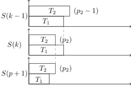
Let k be the last iteration where the algorithm GreedyMappingInt allocates a processor to T2. More formally; k = min{q|alloc(T2) = p2in S(q)}. At
the kthiteration, alloc(T
T1 T2 (p2) S(p + 1) T1 T2 (p2) S(k) T1 T2 (p2− 1) S(k − 1)
Figure 7: Case 2 in the proof of Theorem 2.
We consider the time needed to finish the two subtrees in OP T (p + 1): M Sr(OP T (p + 1)) > completion time of T2 in OP T (p + 1)
> M S(T2(p∗2))
> M S(T2(p2− 1)) as p∗26 p2− 1
> M Sr(S(k − 1)) (T2 is the last task in S(k − 1))
> M Sr(S(k))
> M Sr(S(p + 1))
The last inequality is valid as adding processors will not give a longer makespan: we assume that the function fi(k), that gives the duration of
node i on k processors, is non-decreasing.
As OP T and S(p + 1) allocate p + 1 processors to the root, we conclude that M S(OP T (p + 1)) > M S(S(p + 1)), and this contradicts the fact that S(p + 1) is not optimal (see Figure 7).
Case 3: p1+ 1 > p∗1 In this case p1+ 1 > p∗1. So, p1> p∗1.
Then,
M Sr(OP T (p + 1)) > completion time of T1 in OP T (p + 1)
> M S(T1(p∗1))
> M S(T1(p1)) as p1> p∗1
So, M Sr(OP T (p + 1)) > M Sr(S(p + 1)), because both schedules allocate
p+1 processors to the root. Therefore, M S(OP T (p+1)) > M S(S(p+1)), which contradicts the fact that S(p + 1) is not optimal.
We conclude that the algorithm GreedyMappingInt is optimal with p + 1 pro-cessors.
We now prove that the algorithm GreedyMappingInt is also optimal on gen-eral trees.
Proof 2 (Theorem 1) The proof is similar to the previous one. Instead of having two subtrees, we consider the k subtrees T1, T2, · · · , Tk of the root.
W.l.o.g., we suppose that during the p + 1thstep, GreedyMappingInt allocates
the last processor to T1. Three cases are distinguished and treated as follows.
Case 1 S(p+1) and OP T (p+1) allocate the same number of processors to each subtree. In this case, the induction hypothesis is used as in the previous proof.
Case 2 OP T allocates more processors to a subtree T1 (p∗1 > p1 + 1). In
this case, there is at least another subtree Ti where OP T allocates less
processors than S(p+1) (p∗i < pi). We use the same analysis as the second
case of the previous proof by changing T2into Ti.
Case 3 OP T allocates less processors to the subtree T1 (p∗1 < p1+ 1). In this
case, the exact same analysis used in the third case of the previous proof can be performed.
Inovallée
655 avenue de l’Europe Montbonnot
BP 105 - 78153 Le Chesnay Cedex inria.fr


![Table 1: Set of real-life matrices issued from The SuiteSparse Matrix Collec- Collec-tion [5] (except matr5 and lap120), sorted by family and number of operaCollec-tions.](https://thumb-eu.123doks.com/thumbv2/123doknet/12962364.376917/16.918.165.672.320.883/table-matrices-issued-suitesparse-matrix-collec-collec-operacollec.webp)