Hierarchical Finite-State Modeling for Texture Segmentation with Application to Forest Classification
Texte intégral
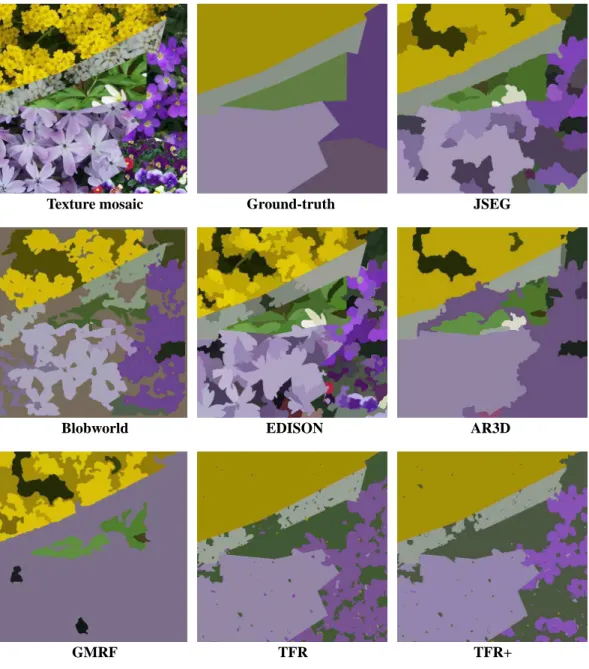
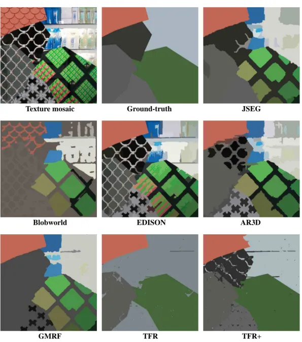
Figure


Documents relatifs
The two bold black lines represent marginal curves of declination and inclination of the obtained secular variation reference curve for Austria surrounded by their 95 per cent
L’archive ouverte pluridisciplinaire HAL, est destinée au dépôt et à la diffusion de documents scientifiques de niveau recherche, publiés ou non, émanant des
given resource, or between two different actors & justify his/her suggestion (type of information used by actors?). Each arrow/interaction is characterized by an
In this study, considering the energy performance, the final energy consumption for heating forms an objective vector, thereby objective space.. The others compose
CONTEXT-BASED ENERGY ESTIMATOR The idea of snakes or active contours [2] is to evolve a curve under the influence of internal forces coming from the curve itself and of external
We compare the use of the classic estimator for the sample mean and SCM to the FP estimator for the clustering of the Indian Pines scene using the Hotelling’s T 2 statistic (4) and
On the use of a Nash cascade to improve the lag parameter transferability at different
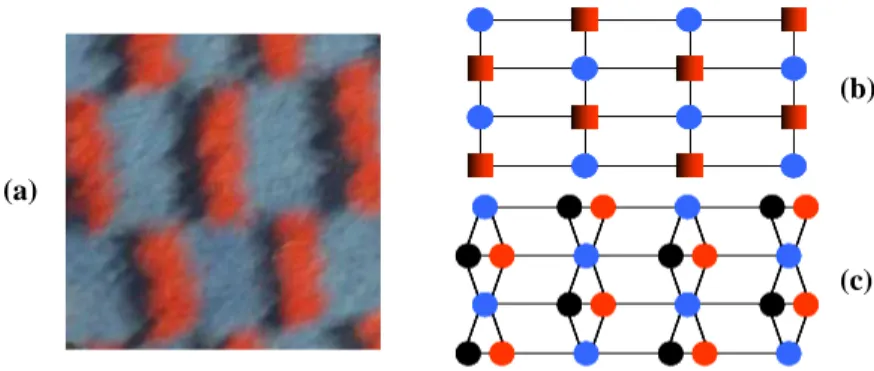
Moreover, these reduced basis have been used sucessfully to calculate the electronic structure of the molecules. Each atom of carbon has four nearest neighbours and
