Accelerating Magnetic Resonance Imaging by
Unifying Sparse Models and Multiple Receivers
by
Daniel S. Weller
B.S., Carnegie Mellon University (2006)
S.M., Massachusetts Institute of Technology (2008)
Submitted to the Department of Electrical Engineering and Computer
Science
in partial fulfillment of the requirements for the degree of
Doctor of Philosophy in Electrical Engineering
at the
MASSACHUSETTS INSTITUTE OF TECHNOLOGY
June 2012
@
2012 Massachusetts Institute of Technology. All rights reserved.
Author ...
-Department of Electrical Engineering and Computer Science
I/ /
Certified by...
7fMarch 30, 2012
...Vivek K. Goyal
Associate Professor of Electrical Engineering and Computer Science
Thesis Supervisor
Accepted by ...
Professor eslie
.
Stolodziejsi
Chair, Committee on Graduate Students
ARCHIVES
MNASISEA T S INSTTUTEAccelerating Magnetic Resonance Imaging by Unifying
Sparse Models and Multiple Receivers
by
Daniel S. Weller
Submitted to the Department of Electrical Engineering and Computer Science on March 30, 2012, in partial fulfillment of the
requirements for the degree of
Doctor of Philosophy in Electrical Engineering
Abstract
Magnetic resonance imaging (MRI) is an increasingly versatile diagnostic tool for a variety of medical purposes. During a conventional MRI scan, samples are acquired along a trajectory in the spatial Fourier transform domain (called k-space) and the image is reconstructed using an inverse discrete Fourier transform. The affordability, availability, and applications of MRI remain limited by the time required to sam-ple enough points of k-space for the desired field of view (FOV), resolution, and signal-to-noise ratio (SNR). GRAPPA, an accelerated parallel imaging method, and compressed sensing (CS) have been successfully employed to accelerate the acquisi-tion process by reducing the number of k-space samples required. GRAPPA leverages the different spatial weightings of each receiver coil to undo the aliasing from the re-duction in FOV induced by undersampling k-space. However, accelerated parallel imaging reconstruction methods like GRAPPA amplify the noise present in the data, reducing the SNR by a factor greater than that due to only the level of undersampling. Completely separate from accelerated parallel imaging, which capitalizes on observ-ing data with multiple receivers, CS leverages the sparsity of the object along with incoherent sampling and nonlinear reconstruction algorithms to recover the image from fewer samples. In contrast to parallel imaging, CS actually denoises the result, because noise typically is not sparse. When reconstructing brain images, the discrete wavelet transform and finite differences are effective in producing an approximately sparse representation of the image. Because parallel imaging utilizes the multiple re-ceiver coils and CS takes advantage of the sparsity of the image itself, these methods are complementary, and a combination of these methods would be expected to enable further acceleration beyond what is achievable using parallel imaging or CS alone.
This thesis investigates three approaches to leveraging both multiple receiver coils and image sparsity. The first approach involves an optimization framework for jointly optimizing the fidelity to the GRAPPA result and the sparsity of the image. This technique operates in the nullspace of the data observation matrix, preserving the ac-quired data without resorting to techniques for constrained optimization. While this framework is presented generally, the effectiveness of the implementation depends on
the choice of sparsifying transform, sparsity penalty function, and undersampling pat-tern. The second approach involves modifying the kernel estimation step of GRAPPA to promote sparsity in the reconstructed image and mitigate the noise amplification typically encountered with parallel imaging. The third approach involves imposing a sparsity prior on the coil images and estimating the full k-space from the observa-tions using Bayesian techniques. This third method is extended to jointly estimate the GRAPPA kernel weights and the full k-space together. These approaches rep-resent different frameworks for accelerating MRI imaging beyond current methods. The results presented suggest that these practical reconstruction and post-processing methods allow for greater acceleration with conventional Cartesian acquisitions. Thesis Supervisor: Vivek K. Goyal
Acknowledgments
My deepest thanks go to my parents, Jay and Leslie, and my brother, Brian, for being
so supportive of me. From an early age, my parents encouraged me to be inquisitive and nurtured my passion for math and science. Good-natured competition with my brother helped prepare me for a demanding academic career. It is to my family that
I dedicate this thesis.
There are so many here at MIT that made my experience here fulfilling. Vivek and the members of the STIR group, past and present, provided countless hours of advice, support, and encouragement. Julius, who finished his PhD in the group around the same time that I arrived in 2006, proved on my earliest days of graduate school that one can succeed through hard work. I am grateful to my fellow students, Adam, Andrea, Ha, John, Joong, Kirmani, Lav, Mike, Vahid, and Vinith, and the group's many visitors, including Aniruddha, Aycan, BJ, G6tz, Jos6, Pier Luigi, Ulugbek, and Woohyuk, for all the stimulating discussions and meetings over the last six years and just generally sticking together and making research so much fun!
Similarly, Elfar's MRI group, including Audrey, Berkin, Borjan, Div, Filiz, Jes-sica, Joonsung, Lohith, Obaidah, Shao Ying, and Trina, and my collaborators at
MGH, including Fa-Hsuan, Larry, Jon, Kawin, Kyoko, and Thomas, were wonderful
colleagues and friends who made available their vast knowledge to help me realize this thesis. Additionally, I express my sincerest gratitude to Leo at Siemens Corporate Research, for enthusiastically supporting my research, despite the hundreds of miles that separated us.
Many student groups influenced me during my time here. My colleagues and friends in the EECS GSA and in the Sidney Pacific House Council provided endless fun and enjoyment throughout my time here. I also enjoyed my involvement in the Graduate Student Council, and I thank Gerald, Leeland, and Alex for their encouragement. I cherish my friendships with Dennis, Tom, and others in the DSP Group, and playing tennis and games with Da, Ligong, and others from the sixth floor has been an excellent diversion.
I thank Professor Dahleh and Professor Oppenheim for their advice and support
through all these years. Professor Dahleh helped guide me through my studies here at MIT and ensured that I did not overlook any of the requirements. Professor Oppenheim organized a graduate mentoring seminar for new students in my first year, including me, and helped cultivate a collegial atmosphere that made MIT a much warmer and less intimidating place. I also appreciated teaching with Professor Oppenheim, and I greatly enjoyed the experience.
Of course, I also want to thank my friends around MIT and beyond for keeping
me grounded and sane. If not for playing board games or tennis, attending Celtics, Bruins, or Red Sox games, or just going out and having fun together, life beyond research would have been quite dull.
Last, but not least, I extend my utmost gratitude to my thesis committee, includ-ing my supervisor Vivek, and my readers Elfar, Pablo, Larry, and Leo. While not an official member of my thesis committee, Jon also helped extensively to supervise
my research. My experience would not have been nearly so satisfying without your input, comments, and mentoring. The administrative staff, namely Eric, Kathryn, and Gabrielle in STIR, Arlene in the MRI group, and the technologists and support staff at MGH, also played critical roles throughout the research process. Thank you for your assistance, support, and friendship.
On a less personal note, this research was supported by NSF CAREER Award
CCF-0643836, Siemens Healthcare, NIH R01 EB007942 and EB006847, NIH NCRR
P41 RR014075, and NDSEG and NSF Graduate Research fellowships. Daniel S. Weller
Contents
1 Introduction 17
1.1 Outline... ... 20
1.2 Bibliographical Notes . . . . 23
2 Magnetic Resonance Imaging 25 2.1 M R Physics . . . . 25
2.2 Cartesian MR Imaging . . . . 29
2.3 Accelerated MR Imaging . . . . 33
2.4 Parallel MR Imaging . . . . 34
2.5 Accelerated Parallel Imaging Reconstruction . . . . 38
3 Sparsity and Compressed Sensing 47 3.1 Measures of Sparsity . . . . 48
3.2 Sparsity-Based Denoising . . . . 52
3.3 Compressed Sensing Reconstruction . . . . 55
3.4 Compressed Sensing for MRI . . . . 59
4 Denoising GRAPPA with Sparsity 63 4.1 T heory . . . . 64
4.2 Simulations and Results . . . . 69
4.3 D iscussion . . . . 87
5 GRAPPA Kernel Calibration with Sparsity 91 5.1 Theory... ... 92
5.2 Simulations and Results . 5.3 Discussion . . . . 6 Estimation Using GRAPPA
6.1 Theory... 6.2 Simulations and Results . 6.3 Discussion . . . . . . . . . . . . and Sparsity ... . . . . . . . . 7 Conclusion A Optimization Methods
A.1 Least-Squares Problems ...
A.2 Compressed Sensing Problems . . . . 97 105 109 110 118 121 125 131 131 136
List of Figures
2.1 While the magnetization M is at an angle to the magnetic field Bok, the derivative of the magnetization dM/dt is perpendicular to M, causing the magnetization vector to precess around the magnetic field. ... 27
2.2 RF slice-selective excitation (in z-direction) followed by Cartesian sam-pling of k-space in k.,k,-plane using x- and y-gradients. The acquisition is repeated for different magnitudes of Gy, resulting in the sampling of different phase encode scan lines, shown in the k-space plot on the right. The samples are taken during the frequency encoding x-gradient
and are marked with the ADC. . . . . 31 2.3 The sample spacing Akx in k-space and the extent kx,mx. relate to the
FOV FOVx and voxel size Ax, respectively, of the reconstructed image in the x-direction. Similarly, Ak, and ky,m. are connected to FOV, and A y. . . . . 32
2.4 Uniform undersampling results in coherent aliasing, while non-uniform or random sampling results in incoherent aliasing. Images shown for k-space undersampled by a factor of 4, with zero-filling reconstruction. 34
2.5 This 96-channel head array coil prototype has many small coils (metal
rings) around the head enclosure. Each coil has its own data acqui-sition hardware, so all the channels can be acquired simultaneously. Commercially available array coils enable parallel imaging to be used for many MRI applications. . . . . 35
2.6 Block diagram of the observation model for an MRI acquisition with
a P-channel parallel receive array coil. The sensed magnetizations
Mi(r),..., Mp(r) all derive from the object magnetization M(r). The k-space observations yi [k], ... ,yp[k] are generated simultaneously from
these sensed magnetizations. . . . . 36 2.7 Magnitude coil sensitivities for 32-channel head coil array computed
from acquired data using 32-channel array and single-channel body coils. 37
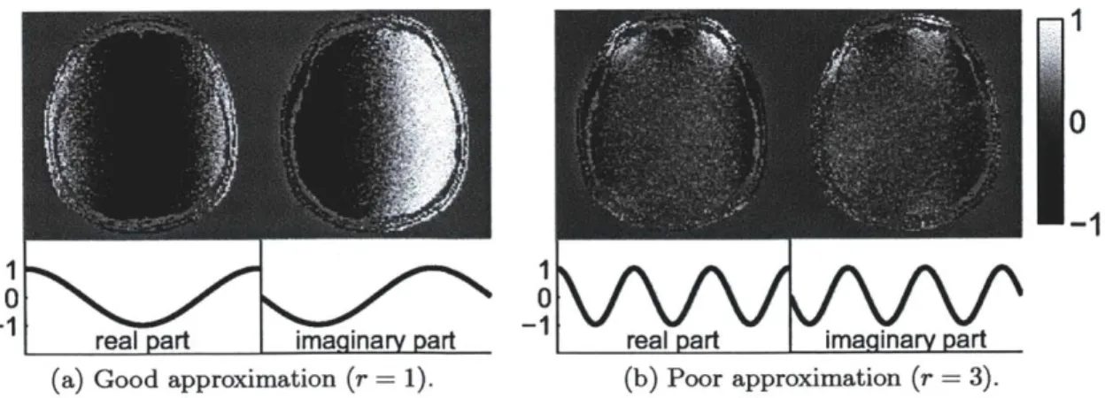
2.8 Real and imaginary parts of SMASH approximations (top) to complex
exponentials (bottom) using a least-squares fit with empirical sensitiv-ities of a 32-channel head coil receive array . . . . 41
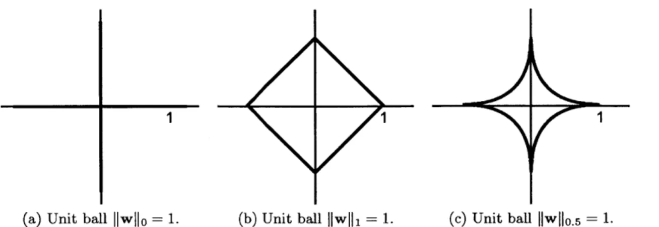
3.1 Unit balls are shown in two dimensions for the fo, f1, and f, measures. Note that the two lines that form the two-dimensional unit ball for the
fo "norm" actually extend to ±oo and exclude the origin. . . . . 49
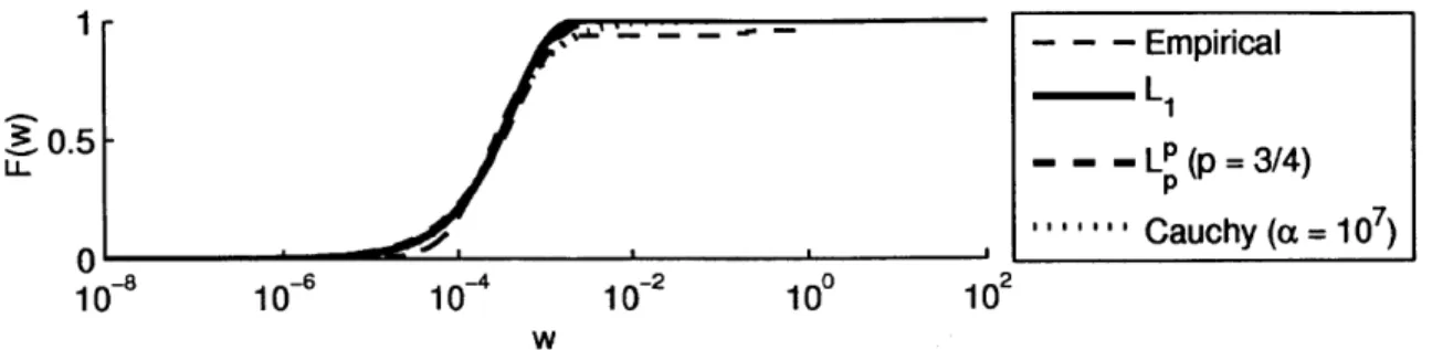
3.2 The f1 norm is plotted with PP "norms" for different values of p (0 < p < 1). The fo "norm" is included for comparison. . . . . 49
3.3 The Cauchy penalty function is plotted for different values of a. The fo "norm" is included for comparison. . . . . 50
3.4 K-space undersampling patterns and their point spread functions. . . 60
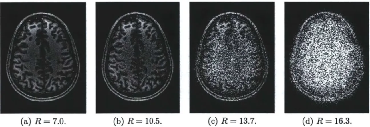
4.1 GRAPPA reconstructions for 2-D uniformly spaced (a) 3 x 3, (b) 4 x 4, (c) 5 x 5, and (d) 6 x 6 nominal undersampling with increasing total acceleration factor R and a 32-channel coil at 3 T. . . . . 63
4.2 Ground truth magnitude images of real ((a)-(c)) and synthetic
((d)-(f)) datasets. Inset regions (white rectangles) are used later to show
detail. ... ... . . ... ... .... . 70
4.3 Sparsity model cdf's for the transform coefficient magnitudes of a Shepp-Logan phantom in the finite differences domain. . . . . 73
4.4 Sparsity model cdf's for the transform coefficient magnitudes of a Tr weighted real image in the four-level '9-7' DWT domain. . . . . 73
4.5 Continuation scheme parameters studied for DESIGN denoising of T1
-weighted image #1 (4 x 4 nominal undersampling: R = 10.5) using
the Cauchy penalty function with four-level '9-7' DWT. . . . . 74 4.6 DESIGN denoising of Shepp-Logan phantom (4 x 4 nominal
undersam-pling: R = 8.7) using fl, PP, and Cauchy penalty functions with the
finite differences representation. . . . . 75
4.7 DESIGN denoising of Ti-weighted image (4 x 4 nominal undersampling:
R = 10.5) using fl, EP, and Cauchy penalty functions with the
four-level '9-7' DW T. . . . . 75
4.8 Trend in the optimal choice of A as determined by coarse-then-fine parameter sweeps for the f1 norm and Cauchy penalty functions, for the
T-weighted image #1 with four-level '9-7' DWT sparsifying transform. The nominal undersampling increases from 3 x 3 (R = 7.0) to 6 x 6
(R = 16.3). . . . . 76
4.9 Reconstructed images (top row) and difference images (bottom row) for
DESIGN denoising with f1 and Cauchy penalty functions compared to
GRAPPA, GRAPPA with Wiener filter-based denoising, CS with joint sparsity and both Li and Cauchy penalty functions, and L1 SPIRiT for
R = 10.5 undersampled T-weighted image #1 with four level '9-7'
DWT sparsifying transform. . . . . 78
4.10 Reconstructed images (top row) and difference images (bottom row) for
DESIGN denoising with f1 and Cauchy penalty functions compared to
GRAPPA, GRAPPA with Wiener filter-based denoising, CS with joint sparsity and both f1 and Cauchy penalty functions, and L1 SPIRiT for
R = 10.5 undersampled Ti-weighted image #2 with four level '9-7'
4.11 Reconstructed images (top row) and difference images (bottom row) for DESIGN denoising with f1 and Cauchy penalty functions compared to GRAPPA, GRAPPA with Wiener filter-based denoising, CS with joint sparsity and both f1 and Cauchy penalty functions, and L1 SPIRiT for R = 14.6 undersampled T2-weighted image with four level '9-7' DWT
sparsifying transform. . . . . 79
4.12 Estimated g-factors (in dB) are plotted for Ti-weighted image #1 with
R = 10.5 acceleration factor (4 x 4 nominal undersampling). . . . . . 82
4.13 Synthetic contrast phantom reconstructions using GRAPPA and de-noising methods (4 x 4 nominal undersampling: R = 12.1) with a four-level '9-7' DWT sparsifying transform. . . . . 83
4.14 Synthetic resolution phantom reconstruction comparisons of effective spatial resolutions using GRAPPA and denoising methods (4 x 4 nom-inal undersampling: R = 12.1) with a four-level '9-7' DWT sparsifying
transform . . . . 84 4.15 GRAPPA and DESIGN denoising methods compared for uniform and
random undersampled (4 x 4 nominal undersampling: R = 8.7) Shepp-Logan phantom with finite differences sparsifying transform. ... 86
4.16 GRAPPA and DESIGN denoising methods compared for uniform and Poisson disc random undersampled (5 x 5 nominal undersampling:
R f 13.7) Ti-weighted MPRAGE dataset with four-level '9-7' DWT
sparsifying transform. . . . . 88 5.1 GRAPPA reconstructions with low-quality kernel calibrations
demon-strating noise amplification (left) and residual aliasing (right) with 4 x 4 nominal undersampling. The GRAPPA reconstruction on the left was calibrated with 36 x 36 ACS lines and no regularization, and the reconstruction on the right was calibrated with 20 x 20 ACS lines (underdetermined) with Tikhonov regularization. . . . . 92
5.2 GRAPPA reconstructions of T-weighted image #1 (4 x 4 nominal
un-dersampling: R 10.5) with high-quality kernel calibrations with no
regularization, Tikhonov regularization, and sparsity-promoting regu-larization. . . . . 99 5.3 GRAPPA reconstructions of T-weighted images #1 and #2 (4 x 4
nominal undersampling: both R = 10.5) with low-quality kernel cali-brations with no regularization, Tikhonov regularization, and sparsity-promoting regularization. . . . . 100
5.4 GRAPPA reconstructions of 4 x 4 nominally undersampled Ti-weighted image #1 (R = 13.7) and image #2 (R = 12.9) with underdeter-mined kernel calibrations with Tikhonov regularization and sparsity-promoting regularization. . . . . 101 5.5 Trade-off curves for un-regularized, Tikhonov-regularized, and
sparsity-promoting GRAPPA kernel calibration depicting the relationship be-tween reconstructed image PSNR and total acceleration R as the num-ber of ACS lines is varied. Nominal undersampling is held fixed at 4 x 4.103
5.6 Trade-off curves for un-regularized, Tikhonov-regularized, and
sparsity-promoting GRAPPA kernel calibration depicting the relationship be-tween reconstructed image PSNR and total acceleration R as the total acceleration is varied (by varying both nominal undersampling and the number of ACS lines). . . . . 104
5.7 GRAPPA and DESIGN-denoised reconstructions of Ti-weighted image
#2 (4 x 4 nominal undersampling: R = 12.9) with underdetermined sparsity-promoting kernel calibration. . . . . 105 5.8 GRAPPA with un-regularized and sparsity-promoting calibration and
DESIGN-denoised GRAPPA with sparsity-promoting calibration of Ti-weighted image #2 (4 x 4 nominal undersampling: R = 10.5) with 36 x 36 ACS lines. . . . . 106
6.1 Reconstructed and difference images using conventional GRAPPA and Bayesian full k-space estimation for Ti-weighted image #2 for several acceleration factors (nominal undersampling increases from 4 x 3 to
5 x 5). . . . . 120
6.2 Reconstructed and difference images using conventional GRAPPA and
Bayesian joint estimation of the kernel and full k-space for T-weighted image #2 at higher acceleration factors (nominal undersampling 5 x 4 and 5 x 5 for the top and bottom rows, respectively). . . . . 121
6.3 Reconstructed and difference images using conventional GRAPPA and
Bayesian joint estimation of the kernel and full k-space for T-weighted image #2 with a larger GRAPPA kernel (nominal undersampling is 5 x4).122
A.1 Steepest descent (dotted line) and conjugate gradient (solid line)
List of Tables
4.1 Penalty functions and associated sparsity priors on transform coeffi-cient m agnitudes. . . . . 72
4.2 PSNRs (in dB) of reconstruction methods at different acceleration fac-tors for T1-weighted image #1 . . . . 80
4.3 PSNRs (in dB) of reconstruction methods at different acceleration fac-tors for T1-weighted image #2 . . . . 80
4.4 PSNRs (in dB) of reconstruction methods at different acceleration fac-tors for T2-weighted image. . . . . 80
Chapter 1
Introduction
Since its development in the 1970s, magnetic resonance imaging (MRI) has steadily gained in importance to clinicians and researchers for its ability to produce high qual-ity images non-invasively without the side effects of ionizing X-ray radiation. MRI is used extensively to image soft tissue throughout the whole body [22]. Moreover, magnetic resonance imaging can be used to distinguish gray and white matter in the brain, observe blood flow, and measure diagnostically valuable quantities such as cortical thickness [13, 47, 32]. Because of its great versatility, MRI has myriad appli-cations in both medical research and diagnostic and perioperative clinical imaging. However, magnetic resonance imaging remains limited by the time required to gen-erate these images. A typical MRI of a brain can take between five and ten minutes, during which the subject must remain perfectly still. This requirement is a hardship for certain populations like young children, the elderly, and patients experiencing chronic or acute pain. Since many MRI bores are narrow enclosed spaces, subjects may experience claustrophobia, making remaining motionless more difficult. Because multiple scans are typical for many applications, sessions commonly extend beyond one hour in duration, increasing costs and reducing availability of the scanner. In addition, compromises in image quality such as resolution reduction are necessary for time-critical applications like functional MRI [71, 6].
MRI acquisition speed is limited by physiological constraints connected to the effects of spatially varying magnetic fields on the body. A spatially-varying applied
magnetic field can induce currents in the nervous system; at high enough rates, these currents can stimulate the nerves, irritating or distressing the subject [40]. As the fields used to encode the spatial information for Fourier coefficients are spatially vary-ing, this constraint essentially limits the rate we can collect MRI data. Past efforts in accelerating MRI have centered upon adjusting the sampling pattern or acquir-ing multiple samples simultaneously. All these methods have their advantages and disadvantages. Adjusting the sampling pattern often means reducing resolution, los-ing phase information, or requirlos-ing more complicated reconstruction methods [9, 70]. Fast MRI acquisition techniques also can use multiple echoes to reduce imaging time while reducing contrast or increasing susceptibility to magnetic field
inhomogene-ity [62, 41, 30].
A different approach for accelerating MRI uses multiple receivers in parallel and
post-processing to recover complete images from fewer samples. Parallel imaging had already been used effectively to mitigate noise, and now, accelerated parallel imaging methods also enable faster acquisitions [82, 87, 76, 38]. Whereas conventional re-ceiver coils have a single channel with spatially uniform sensitivity to magnetization, parallel receiver coils have multiple channels with different non-uniform magnetic sen-sitivities [82]. Accelerated parallel imaging reconstruction methods use the different sensitivities of the coil channels to resolve the ambiguity due to undersampling [76]. Such methods already are popular in commercial scanners, enabling modest levels of acceleration for many types of imaging, but these methods alone are insufficient for the high acceleration levels we would like to attain.
Another technique for reconstructing images from undersampled data called com-pressed sensing (CS) emerged in the signal processing community [18, 16, 20, 27]. Compressed sensing takes advantage of the sparsity or compressibility of an appro-priate representation or transform of the desired image. While not specific to MRI, MRI is a widely suitable candidate for CS due to the approximate transform spar-sity of many MR images and the ability to use nearly arbitrary (random) sampling patterns [57]. For instance, many MR images have few edges or have simple textures representable using a small number of wavelet coefficients. CS has enabled successful
reconstructions of modestly accelerated MRI data [57].
By combining the sparsity models with the accelerated parallel imaging
recon-struction methods already developed, we expect high quality reconrecon-structions from data collected with even greater undersampling. Linear system inversion techniques for accelerated parallel imaging reconstruction like SENSE [76] and SPIRiT [59] can be directly combined with the compressed sensing reconstruction framework. Methods like SparseSENSE [52] and Li SPIRiT [56] follow this approach, yielding a sparsity-promoting regularized reconstruction method that can recover high quality images
from moderate accelerations with random undersampling.
With conventional uniform undersampling, we aim to improve the auto-calibrating kernel-based interpolation method GRAPPA [38]. As a direct method (not an inver-sion), this reconstruction approach cannot be directly incorporated into a compressed sensing framework. Further complicating the combination with sparse models is the two-step formulation of the GRAPPA method: both the calibration and interpolation steps influence the reconstruction quality and can introduce noise or artifacts. Also, while theoretical results concerning compressed sensing rely on a random or pseudo-random observation matrix, the observations are uniformly spaced, yielding coherent aliasing that cannot be distinguished based on sparsity alone. In this work, we study three different approaches to improving GRAPPA using sparsity models: denoising the reconstructed image, regularizing the calibration step, and estimating the channel images using Bayesian sparsity models.
We demonstrate that all these approaches successfully extend the GRAPPA ac-celerated parallel imaging method to higher accelerations by having either greater spacing between samples, or less calibration data, and yielding high quality images. The denoising method reduces the noise amplification from both undersampling the data and the GRAPPA reconstruction process. The improved calibration method reduces the amount of calibration data needed to produce a quality GRAPPA recon-struction, mitigating the aliasing and noise that would otherwise result. The joint estimation method combines these ideas to reconstruct both the GRAPPA kernel needed for interpolation and the denoised full channel images from the undersampled
data, enabling reconstructions from highly undersampled data with less calibration data. Results using real MRI data are presented that portray the effectiveness of these methods relative to conventional accelerated parallel imaging at high levels of acceleration. We conclude from these results that significant gains in both image quality and total acceleration can be made using all three of these methods, enabling much faster MRI scans with currently employed image acquisition paradigms.
1.1
Outline
Effective combination of accelerated parallel imaging methods with compressed sens-ing requires an in-depth understandsens-ing of the advantages and drawbacks of each. Keeping in mind the strengths and weaknesses of these methods, we propose three distinct approaches to combining GRAPPA, a widely-used accelerated parallel imag-ing method, and image sparsity. We introduce a denoisimag-ing method that mitigates noise amplification at moderate levels of acceleration. We also propose a sparsity-promoting auto-calibration method for GRAPPA that enables significantly greater acceleration by reducing the amount of calibration data needed. Finally, we con-sider a Bayesian estimation-theoretic framework for jointly calibrating the GRAPPA reconstruction method and reconstructing denoised full images from undersampled data. We conclude this thesis with a discussion of the merits and drawbacks of the proposed methods and their respective places in practical accelerated imaging.
Background on magnetic resonance imaging is presented in Chapter 2. We begin with a basic discussion of MR physics, emphasizing the classical aspects leading up to the signal equation, which describes the connection between the magnetic moments, fields, and the measured received signal. Connections between the sampling of k-space and the spatial resolution and field of view of the image are drawn. Methods for accelerating MRI acquisition, including partial Fourier imaging and fast pulse echo sequences are described, ending with an introduction to accelerated parallel imaging. Techniques for combining coil images and measuring coil sensitivities are presented, and important pre-existing accelerated parallel imaging reconstruction techniques are
described in detail. The nullspace formulation of SPIRiT is presented as an example of this constrained optimization method that proves useful later.
In Chapter 3, sparsity models and the compressed sensing framework are de-scribed in detail. The notions of sparsity, transform sparsity, and compressibility are developed, and measures of sparsity, including the
eo,
f1, and(
measures, are pre-sented. An introduction to joint and group sparsity and appropriate hybrid measures follows. Linear and nonlinear methods for sparsity-based denoising are introduced and extended to the joint sparsity case. Once these preliminaries are complete, thecompressed sensing framework is developed, and key theoretical concepts like the re-stricted isometry property and mutual coherence are explained. Compressed sensing is then applied to the problem of reconstructing MRI images from undersampled data, and major results from the literature are described. Additional time is spent depicting sampling patterns for compressed sensing MRI used in the literature. This chapter concludes with a discussion of the literature combining compressed sensing with ex-isting accelerated parallel imaging reconstruction methods and how these methods differ from the contributions in this thesis.
As mentioned earlier, three approaches for improving GRAPPA accelerated par-allel imaging using sparsity models are proposed. The first approach, denoising the GRAPPA result using sparsity, is described in Chapter 4. Motivating this develop-ment is the preponderance of noise present in GRAPPA reconstructed images at high accelerations. The proposed method aims to reduce the noise to a more acceptable level by adjusting the interpolated (missing) k-space frequencies to promote the joint transform sparsity of the coil images. A few innovations are made: the nullspace method is applied to preserve the acquired data while denoising the coil images; the GRAPPA result is used directly, saving on computation; and the method is developed with the explicit goal of denoising, not requiring any deviation from conventional uni-form undersampling. The complete method also considers the contribution of each voxel in each coil channel to the final combined image, allowing for greater deviation from the GRAPPA reconstruction in those voxels deemed too noisy or too insignifi-cant in the combined image.
A variety of studies are performed on real and simulated data using this denoising
method. Interpreting the choice of sparsity-promoting regularization penalty as im-posing a prior distribution on the sparse transform coefficients, the empirical cumula-tive distribution function (cdf) of the combined reference image transform coefficients is compared to the distributions for a variety of penalty functions, and denoising is performed using all these penalties to visualize the effects of imposing an appropriate prior on the denoised image. First performed for the Shepp-Logan phantom, this experiment is repeated for real MRI data.
Additional experiments depict the impact of continuation scheme parameters and the tuning parameter on the denoising quality. A series of comparisons are performed to portray differences in image quality, noise suppression, and contrast/resolution degradation among the proposed method and existing reconstruction and denoising methods. The chapter concludes with a depiction of denoising adapted to differ-ent sampling patterns and a discussion of the advantages and disadvantages of the proposed method that can be inferred from these experiments.
A second approach utilizes sparsity to regularize the GRAPPA kernel
calibra-tion step. In Chapter 5, this improved calibracalibra-tion method is derived and compared to un-regularized and conventionally regularized kernel calibration. Using real MRI reference images, reconstructions are performed using different numbers of ACS cali-bration data, and the impact of different kinds of regularization is portrayed in these experiments. Since varying the number of ACS lines can be interpreted as trading image quality for greater total acceleration, the trade-off curves for these different calibration methods are plotted, and the improvement in the achievable trade-off region is significant. This chapter ends with experiments depicting the additional improvement from post-processing the regularized GRAPPA method with the de-noising method proposed in the previous chapter. From the improvement visible in these last experiments, we speculate that additional gains are possible from combining the calibration and reconstruction/denoising steps when regularizing with sparsity.
We investigate this combination of calibrating the GRAPPA kernel and recon-structing the full k-space in Chapter 6. We begin by formulating a Bayesian
esti-mation problem using both the acquired data and the GRAPPA reconstructions as observations (with different noise models) and treating the joint transform sparsity as a prior distribution on the full k-space across all the coil channels. After deriving the posterior-maximizing estimator for this problem, we consider how the estimation problem changes when the GRAPPA kernel is a variable. The transformed problem enables joint estimation of both the kernel and the full coil-by-coil k-space from the acquired data (including ACS lines). This problem is solved by adapting the iterative algorithms used in previous chapters to compute the denoised full k-space and regu-larized GRAPPA kernel. Experiments on real data depict significant improvements in image quality at very high accelerations, even when using relatively little calibra-tion data. From these experiments, we conclude that this joint estimacalibra-tion method,
by combining the effects of sparsity models on the calibrated kernel and on the full
k-space, enables high quality imaging from even less data than before.
In Chapter 7, we conclude by summarizing the conclusions and contributions made in these chapters, and we follow this summary by a discussion of the impact on the field and what future directions may enable even greater improvements in accelerated MR imaging.
1.2
Bibliographical Notes
Parts of Chapter 4 appear in papers:
" D. S. Weller, J. R. Polimeni, L. Grady, L. L. Wald, E. Adalsteinsson, and
V. K. Goyal. Denoising sparse images from GRAPPA using the nullspace method (DESIGN). Magn. Reson. Med., to appear (available online, DOI:
10.1002/mrm.24116). PubMed Central PMID: 22213069.
" D. S. Weller, J. R. Polimeni, L. Grady, L. L. Wald, E. Adalsteinsson, and V. K.
Goyal. Combined compressed sensing and parallel MRI compared for uniform and random Cartesian undersampling of k-space. In Proc. IEEE Int. Conf.
" D. S. Weller, J. R. Polimeni, L. Grady, L. L. Wald, E. Adalsteinsson, and V. K.
Goyal. SpRING: Sparse reconstruction of images using the nullspace method and GRAPPA. In Proc. ISMRM 19th Scientific Meeting, page 2861, May 2011.
" D. S. Weller, J. R. Polimeni, L. Grady, L. L. Wald, E. Adalsteinsson, and V. K.
Goyal. Evaluating sparsity penalty functions for combined compressed sensing and parallel MRI. In Proc. IEEE Int. Symp. on Biomedical Imaging, pages
1589-92, March-April 2011.
" D. S. Weller, J. R. Polimeni, L. Grady, L. L. Wald, E. Adalsteinsson, and V.
K. Goyal. Combining nonconvex compressed sensing and GRAPPA using the nullspace method. In Proc. ISMRM 18th Scientific Meeting, page 4880, May 2010.
Parts of Chapter 5 appear in papers:
" D. S. Weller, J. R. Polimeni, L. Grady, L. L. Wald, E. Adalsteinsson, and V.
K. Goyal. Greater Acceleration through Sparsity-Promoting GRAPPA Kernel Calibration. In Proc. ISMRM 20th Scientific Meeting, to appear.
" D. S. Weller, J. R. Polimeni, L. Grady, L. L. Wald, E. Adalsteinsson, and
V. K. Goyal. Regularizing grappa using simultaneous sparsity to recover de-noised images. In Proc. SPIE Wavelets and Sparsity XIV, volume 8138, pages
81381M-1-9, Aug. 2011.
Parts of Chapter 6 appear in the manuscript:
* D. S. Weller, J. R. Polimeni, L. Grady, L. L. Wald, E. Adalsteinsson, and V. K. Goyal. Accelerated Parallel Magnetic Resonance Imaging Reconstruction Using Joint Estimation with a Sparse Signal Model. In preparation.
Chapter 2
Magnetic Resonance Imaging
A thorough understanding of magnetic resonance imaging (MRI) begins with MR
physics, namely the interactions between bulk material and magnetic fields, and the resulting signal received by nearby coils. These concepts can be employed to acquire
2-D or 3-D images that depict the spatial distribution of magnetically susceptible
ma-terials, including biological tissue. An acquisition executes a specific spatial frequency domain sampling pattern, the properties of which are connected to the voxel size and field of view of the reconstructed image. Several approaches for accelerating MRI within this framework also are described here. Conventional imaging is extended to parallel imaging using multiple receiver coils; existing techniques for reconstructing images from accelerated parallel imaging data are explained and compared, including the GRAPPA method, which is used extensively throughout this thesis.
2.1
MR Physics
The basic classical theory underlying MRI derives from the physics governing the interaction between particles in a bulk material and an externally applied magnetic field. These physical laws also govern detection of the magnetization of these particles and allow us to reconstruct an image of the magnetic properties of the bulk material.
A concise, thorough treatment of these concepts is given in [68]. A summary of
2.1.1
Magnetic Moments
At a high level, MRI involves exciting particles in the test subject using a combination of several external magnetic fields and measuring in a nearby receiver coil the resulting signal generated by those particles. Atoms with an odd number of protons or neutrons have "spin," which can be affected by an applied magnetic field. The most prevalent such particle in the human body is the single-proton hydrogen ('H) atom found in both water and hydrocarbons, especially lipids. This abundance is fortunate as the (1H) atom is highly sensitive to applied magnetic fields, so it produces a strong signal that is relatively easily detected. While it is convenient to think of individual atoms in isolation, the structure of the molecule or compound containing these magnetically susceptible atoms impacts the received signal. Since different tissue types contain different densities of different hydrogen-containing molecules, these signal differences create contrast between tissue types useful for generating useful images depicting anatomy or structure.
To consider the effect of a magnetic field on a susceptible particle, it is helpful to consider the "spin" as a vector quantity, called the magnetic moment. In a bulk material such as biological tissue, this vector is often expressed in terms of magneti-zation M, the net magnetic moment per unit volume. The effect of a magnetic field B on the magnetization is described by the differential equation
d M
= M x -yB, (2.1)
dt
where -y is the gyromagnetic ratio of the particle (y = 2r - 4.2576 - 10' rad/s/T for the hydrogen atom [7]). In the presence of a sufficiently strong static magnetic field, such as the main field generated by a permanent or superconducting magnet in an MRI machine, these spins in equilibrium tend to be oriented in the
airection
of that magnetic field. In keeping with convention, we consider the main field to point in the z-direction of our right-handed 3-D coordinate system. In the context of human MRI, the main field is oriented parallel to the bore of the MRI system.y
Figure 2.1: While the magnetization M is at an angle to the magnetic field Bok, the derivative of the magnetization dM/dt is perpendicular to M, causing the magneti-zation vector to precess around the magnetic field.
will precess in the plane normal to that field (called the transverse plane or axial plane) at the frequency w = -yB; when B is the main field Bok, this frequency wo = -Bo
is called the Larmor frequency. For a main field strength of Bo = 3 T, the Larmor
frequency of a hydrogen atom is wo = 127.73 MHz. This precession behavior is
depicted in Figure 2.1.
To simplify later calculations, we often express Equation (2.1) in the reference frame rotating at the Larmor frequency in the transverse plane. In the rotating reference frame,
dM
= M x (yB - wok). (2.2)
dt
When B = Bok, we have = 0. Thus, in the rotating reference frame, we can
ignore the contribution of the main field when considering the effects of other external magnetic fields on the magnetization.
While the spins are precessing, they induce an electromotive force (emf) in a nearby receiver coil. The observed signal from all the spins can be approximated by integrating the transverse magnetization over the entire volume. For convenience, we write the transverse magnetization M, as a complex number with the real part representing the component in the x-direction, and the imaginary part representing
the component in the y-direction. So M., = M_ + jMy. Thus, although the mag-netization vector is real-valued, our measurements will be complex-valued to capture both components of the transverse magnetization conveniently. The phase of this complex-valued quantity contains information about the actual precession frequen-cies of the spins, which can be used to study chemical structure or composition, main field inhomogeneity, and (as we will use later) spatial location of the spins.
2.1.2
Relaxation and Excitation
While precessing, these moment vectors also move towards equilibrium in a process called relaxation. This relaxation occurs in two ways: by losing magnitude in the transverse plane, which is called transverse or T2 relaxation, and by gaining magnitude
in the main field direction, which is termed longitudinal or T relaxation. Both relaxation processes are modeled by exponential decay with time constants T1 and
T2. Let M2,(t) be the magnitude of M projected onto the transverse plane at time t;
this magnitude component decays as M2,(t) = M2,(O)e-/T2. The component of M in
the z-direction M(t) decays as M2(t) = M - (M - Mz(O))e-/1T. The magnitude
M describes the equilibrium magnetization magnitude. Note that the relaxation
time constants T and T2 are often quite different; for gray matter and white matter
in the brain, T1
>>
T2, so the magnetization will appear to disappear in the transverseplane long before it reappears again in the longitudinal direction. Taking relaxation into account, we modify Equation (2.1):
dM M2. i M (M2 M0) (2.3)
dt T2 T2 T1
The differential system in Equation (2.3) is termed the Bloch equations.
Without some way of perturbing the magnetic moments, the magnetizations would all decay to and remain at equilibrium, and imaging would not be possible. Fortu-nately, the cross product in the Bloch equations tells us that at equilibrium, the spins can be "tipped" into the transverse plane by applying a short radiofrequency (RF) pulse perpendicular to the main field with frequency equal to wo. This process of
exciting the spins requires only a short-duration pulse of much smaller magnitude than the main field; however, unlike the main field, this pulse deposits energy into the susceptible particles, heating the tissue. Therefore, care must be taken during excitation to ensure the rate of heating does not exceed the specific absorption rate (SAR) limit of the subject. Fortunately, most subjects are capable of dissipating this heat to avoid tissue damage under normal conditions. Special care must be taken on subjects with metal present, or with homeostasis imbalance, as these conditions can increase the dangers of RF heating on the body. We will only use the same RF excitation pulse that is used in conventional MRJ, so heating will not be affected by the reconstruction methods proposed in this thesis.
2.2
Cartesian MR Imaging
Cartesian MRI refers to acquiring a Cartesian grid of samples of the spatial Fourier transform of the bulk magnetization. This methodology is very common for acquir-ing images and volumes displayacquir-ing local tissue contrast, and many important pulse sequences implement Cartesian imaging. The key element to Cartesian and other Fourier sampling methods is the use of spatial gradient fields during the relaxation of excited spins. As we describe below, the spacing and extent of the Cartesian grid of samples both affect the acquisition time and the field of view and voxel size of the resulting image.
2.2.1
Gradient Fields
While the Bloch equations describe how spins can be excited to allow the bulk magne-tization to be measured, we need to introduce spatial selectivity to identify how that magnetization is spatially distributed and construct an image (or volume). The ap-proaches discussed here utilize gradient magnetic fields that vary linearly in amplitude over space and are parallel (or anti-parallel) to the main field. We parameterize these fields using the spatial gradient G(t) = [G(t), G,(t), G2(t)] = V2,Y,2B2(t). With
r = [x, y, z] is B2(r, t) = (Bo
+
f
G() -r dT). The received signal isy(t)
j
Mx,(r, e )r o] dr, (2.4)where
k(t) = G(-r) dr. (2.5)
Limiting ourselves to time scales t
<
T1, T2, relaxation is insignificant, and the maindynamic in M2, is due to precession, so demodulating by e'"ot yields a constant (in time) M2,(r):
y(t) = Mxv,(r)e-j27rk(t).r dr. (2.6)
We observe that Equation (2.6) describes the spatial Fourier transform of Mxy(r) at spatial frequency k(t). The spatial Fourier transform domain (either 2-D or 3-D) measured this way is called k-space, and the path traced by k(t) is called the k-space trajectory. By carefully choosing G(t) and our sample times, we can sample the 2-D or 3-D spatial Fourier transform at uniformly spaced intervals. These samples are the discrete Fourier transform (DFT) of the discrete image we seek to acquire.
Note: In addition to exciting spins, the RF excitation pulse can be designed to
select a particular 2-D slice of our image by applying a sinc-like pulse in combination with a linear gradient. Designing such pulses is a separate topic (see
[7]),
but it suffices for our discussion that we can design slice-selective excitation pulses for 2-D slices of almost any thickness, position, and orientation. The original MRI design actually used this slice selection approach in all three directions, requiring a separate excitation and relaxation for every voxel in the acquired volume; however, the speed of this approach is fundamentally limited by the excitation and relaxation times and is rarely used.Conventional D Cartesian MRI consists of repeatedly selecting and exciting a
2-D slice and sampling lines of k-space while applying gradient fields during relaxation.
Suppose we wish to acquire a slice parallel to the transverse plane. We apply an RF pulse with a gradient varying linearly in the z-direction to select the slice. Then, we
90* RF4 A A ~ ftA A -)~ ~(-kx
X2i
Xi2X
Gz= Gx G, ADCFigure 2.2: RF slice-selective excitation (in z-direction) followed by Cartesian sam-pling of k-space in kky-plane using x- and y-gradients. The acquisition is repeated for different magnitudes of G,, resulting in the sampling of different phase encode scan lines, shown in the k-space plot on the right. The samples are taken during the
frequency encoding x-gradient and are marked with the ADC.
apply a gradient varying in the y-direction to shift the k-space trajectory in the k,-direction. Finally, we demodulate and sample y(t) while applying a gradient linearly varying in the x-direction. We repeat, changing the amplitude of the gradient varying in the y-direction to select different lines of k-space. Essentially, we are raster-scanning k-space. We denote the x-direction the readout or frequency encode direction because we sample while tracing the k-space trajectory in that direction. We denote the y-direction the (primary) phase encode y-direction, and we denote the z-y-direction the slice encode direction. This acquisition is depicted in Figure 2.2. This approach can be extended to 3-D Cartesian imaging by avoiding slice selection and instead exciting the entire volume and using the gradients varying in both the y- and z-directions to select the scan line in 3-D k-space. Then, we have two phase-encode directions.
2.2.2
Field of View and Spatial Resolution
In designing a Cartesian MRI acquisition, we need to determine appropriate choices of the field of view (FOV) and the spatial resolution (i.e. voxel size). To avoid spatial aliasing artifacts in the image, the FOV should be larger than what we are imaging. The voxel size should be sufficiently small to resolve the smallest features we are
X X X X Ak3 X X X X 2ky,max X-O-OX X X X X X X
2kx,max
4
FOVZFigure 2.3: The sample spacing Ak, in k-space and the extent kx,max relate to the FOV
FOVx and voxel size Ax, respectively, of the reconstructed image in the x-direction.
Similarly, Ak, and ky,max are connected to FOV, and Ay.
interested in observing. The frequency spacing Ak between samples in k-space (in units of inverse distance) is equal to the reciprocal of the FOV: FOV = 1/Ak. The voxel size A is equal to the reciprocal of the extent of k-space (-kmax to kma) that is sampled: A = 1/(2kmax). These parameters are depicted physically in Figure 2.3.
For safety, we cannot arbitrarily increase the magnitude of the gradient fields, so the total acquisition time for Cartesian imaging is proportional to the number and length of the scan lines acquired. A larger FOV or smaller voxels in the phase encode direction necessitates more scan lines, and smaller voxels in the frequency encode direction increases the length of those scan lines. Assuming that we are not limited
by the sampling rate of our analog-to-digital converter (ADC), we note that the
acquisition time is unaffected by the spacing between samples within a scan line, so we can achieve arbitrarily large FOV in the frequency encode direction for free. Thus, we typically choose the frequency encode direction to point in the longest dimension of our volume to minimize the acquisition time, and we oversample k-space in that direction to avoid any possibility of aliasing.
Image quality is also affected by signal-to-noise ratio (SNR); when SNR is too low, tissue contrast and anomalous regions are difficult to distinguish from observation noise. SNR is roughly proportional to acquisition time, so reducing the acquisition time is accompanied by a similar reduction in SNR. The degradation in SNR will be a major concern in reconstructing quality images from accelerated MRI data.
DAY
2.3
Accelerated MR Imaging
Several approaches have become popular for accelerating Cartesian MRI. Keyhole and partial Fourier imaging reduce the extent of k-space that is sampled and use side information to recover the missing regions. Keyhole imaging [93] is a time-series imaging technique used primarily for contrast-enhanced imaging or cardiac imaging, where multiple volumes are collected, and changes of interest are primarily in the low spatial frequencies. A full volume is collected initially, but only low-resolution volumes are collected in subsequent frames, greatly reducing the acquisition time for each frame and increasing the temporal resolution of the technique. The high frequency data in these accelerated frames are substituted from the initial frame, as discussed in [9]. However, keyhole imaging cannot accelerate single-frame imaging like anatomical MRI without substantially reducing spatial resolution.
On the other hand, partial Fourier imaging can be applied to pretty much any acquisition. In partial Fourier imaging, only one half of k-space and a small part of the other half is fully sampled, and complex conjugation or a more sophisticated technique like homodyne processing [70] is utilized to fill in the remaining frequencies. However, partial Fourier techniques cause signal loss when the real-valuedness assumption of the image is violated, which can be caused by a number of factors including chemical shift, field inhomogeneity, blood flow, and the presence of air (e.g. in the sinuses or oral and nasal cavities), iron (e.g. in blood), or other materials with substantially different magnetic susceptibilities. All these variations can introduce valuable phase information that would be lost by assuming the image is real-valued.
A variety of echo train pulse sequences can be used to yield very fast
acquisi-tions. Echo planar imaging (EPI) [62] and its 3-D analogue echo volumar imaging (EVI) [63] utilize a train of gradient echoes to acquire a complete slice using only a single excitation. Other echo train pulse sequences combining gradient and/or spin echoes like GRASE [30] and RARE [41] also achieve fast imaging, although not nearly as fast as techniques based on gradient echoes alone, since RF spin echoes require more time. All these techniques function on the basic premise of acquiring multiple
(a) Uniform undersampling. (b) Random undersampling.
Figure 2.4: Uniform undersampling results in coherent aliasing, while non-uniform or random sampling results in incoherent aliasing. Images shown for k-space undersam-pled by a factor of 4, with zero-filling reconstruction.
scan lines during the same relaxation period. However, the artifacts and distortions that result from these imaging techniques can make echo train pulse sequences not an ideal approach for accelerated imaging. Although the acceleration is limited, these methods are particularly prevalent in several prominent MRI applications, including functional MRI and clinical and surgical neuroimaging.
Finally, we can increase the spacing between scan lines while maintaining the same k-space extent. This accelerated imaging approach maintains spatial resolution while reducing the FOV. When the object is larger than the reduced FOV, aliasing results, which may make the image unusable. As portrayed in Figure 2.4, uniformly undersam-pling k-space (keeping the spacing between scan lines equal) yields strongly coherent artifacts in the image domain, while non-uniformly (or randomly) undersampling k-space yields incoherent artifacts that appear lower in magnitude but more smeared throughout the image. As is discussed later, parallel imaging can be employed to undo coherent aliasing, and compressed sensing can resolve incoherent aliasing.
2.4
Parallel MR Imaging
Parallel MRI [82] was conceived to use multiple receiver coils to improve image quality
by increasing SNR. Averaging P measurements of k-space improves SNR by a factor
of vT, assuming equal noise variances and ignoring correlations across the coils. Instead of a single large receiver coil surrounding the entire FOV, an array of small coils is used, and ideally, each of these coils senses the magnetizations independently
Figure 2.5: This 96-channel head array coil prototype has many small coils (metal rings) around the head enclosure. Each coil has its own data acquisition hardware, so all the channels can be acquired simultaneously. Commercially available array coils enable parallel imaging to be used for many MRI applications.
of the others. In reality, these coils are coupled due to the shared effects of the induced fields of one coil affecting the others, and as an end result, the noise is correlated to a small degree. Multi-channel receive coil arrays such as the 96-channel head coil [100] shown in Figure 2.5 are now widely available for a multitude of imaging applications. To understand how parallel imaging can be useful for accelerated imaging with reduced-FOV data, we return to the signal equation (Equation (2.6)). With a single coil, we assume the coil senses the entire field of view uniformly, so that the "receive field" B7 is constant. With parallel imaging, the arrays are designed so that the individual coils have highly non-uniform spatial sensitivities. Denote by S,(r) the transverse components of the receive field of the pth coil (that coil's sensitivity); as is done with the transverse magnetization, the two components are combined into a single complex-valued number. Then, the signal y,(t) observed by the pth coil is
yt)= M2,(r)S,(r)e-j27rk(t).r dr. (2.7)
For convenience, we drop the transverse magnetization subscript and write M(r)
M2,(r). Also, when referring to the magnetization sensed by the pth coil, we use the
notation M,(r) = M(r)S,(r).
Each receive channel in the coil array is sampled at the same time, yielding es-timates at the same k-space frequencies k according to Equation (2.7). The sample
Ak
X Mi(r) CTFT y1[k]
Si(r) ni[k] r = [, y, z]
M(r)- k = [kx, ky, kz]
Sp(r) np[k]
Ak = [Akx, Aky, Akz]
X Mp(r) CTFT yp[k]
Figure 2.6: Block diagram of the observation model for an MRI acquisition with a P-channel parallel receive array coil. The sensed magnetizations M1 (r), . . ., Mp(r) all
derive from the object magnetization M(r). The k-space observations y[k], ... , yp[k]
are generated simultaneously from these sensed magnetizations.
y,[k] represents the value of k-space at frequency k; these samples are corrupted by
correlated observation noise, which is modeled by additive complex Gaussian noise
n,[k]. The noise vector [n1[k],... , np[k]]T has covariance A, independent of k. The
observation model for parallel imaging with a P-channel coil is illustrated in in Fig-ure 2.6. Given sufficiently many samples, the inverse DFT can be used to recover the noisy discretized samples M,[r] of the sensed magnetization from y,[k], and any number of coil combination methods can be used to form a combined image M[r].
2.4.1 Coil Sensitivity Estimation
In the far field (the distance is much greater than the radius of the coil), the magnitude of the sensitivity is inversely proportional to the square of the distance. In the near field, the coil can be treated as a series of finite elements, and the Biot-Savart law can be used to simulate the spatial sensitivity of the coil parameterized by curve C:
/
di xB(r) cc f 3 , (2.8)
where £ is the tangent vector on the curve, in the direction of the current flow, and r is the vector from the coil element to the spatial point in question. A simula-tor for estimating sensitivities of arbitrary coil array geometries can be downloaded from
[53].
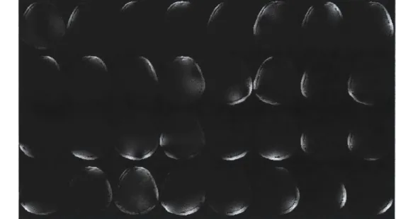
Note that neither the Biot-Savart law nor this simulator account for theFigure 2.7: Magnitude coil sensitivities for 32-channel head coil array computed from acquired data using 32-channel array and single-channel body coils.
dynamic loading and cross-talk that occurs across coils. In addition, the sensitivities are themselves affected by the subject's magnetization. Thus, sensitivities are best determined empirically, with the subject in the magnet.
Multiple approaches exist for empirical measurements. One such measurement di-vides each coil image by the sum-of-squares combined image to yield an estimate of the sensitivities without any additional data; this measurement is derived from compar-ing the sum-of-squares combination to the SNR-optimal formula (see Equations (2.9) and (2.10) below). However, this approach assumes that all the phase information belongs to the coils, so the result is not suitable for reconstructing complex-valued images. If a single-coil acquisition is available, the coil sensitivities can be derived
by dividing the coil images by that single-coil image. Since coil sensitivities are
usu-ally slowly-varying at main field strengths up to 3 T, low-resolution acquisitions and polynomial fitting can be used to improve the robustness of the sensitivity estimation to noise in the single-coil image and regions with low signal (e.g. near the periph-ery of the FOV). An example of high-quality magnitude sensitivity maps estimated from empirical 32-channel and single-channel coil data is shown in Figure 2.7. These sensitivities depict smooth far field decay and higher-order effects like coil loading.