Aerospace composite manufacturing cost models as geometric programs

AEROSPACE COMPOSITE MANUFACTURING COST MODELS

AS GEOMETRIC PROGRAMS by

Scott T. Nill

B. Eng. Vanderbilt University, 2012 S.M. Massachusetts Institute of Technology, 2014 Submitted to the Department of Mechanical Engineering in partial fulfillment of the requirements for the degree of

Doctor of Philosophy at the

MASSACHUSETTS INSTITUTE OF TECHNOLOGY June 2018

2018 Scott T. Nill. All rights reserved.

The author hereby grants to MIT permission to reproduce and to distribute publicly paper and electronic copies of this thesis document in whole or in part in any medium now known or hereafter created.

A uthor...

Signature redacted

C ertified by...

C ertified by ...

...

Department of Mechanical Engineering

If /11, A May 1 1, 20 18

Signature redacted

_...

Wa en Hoburg Visiting Prof s6r, Departmentpf Aeronauti and stronautics hesis Advisor 'I

Ral

lgnature reaactea

_...

David Hardt ph E. and Eloise F. Cross Professor of Mechanical Engineering Chair, Thesis Committee

Signature redacted

A ccepted by ...

Rohan Abeyaratne Quentin Berg Professor of Mechanics Chair, Committee on Graduate Students, Department of Mechanical Engineering

MASSACHUSETTS INSTITUTE

Aerospace Composite Manufacturing Cost Models as Geometric Programs

by

Scott T. Nill

Submitted to the Department of Mechanical Engineering on May 11, 2018, in partial fulfillment of the

requirements for the degree of Doctor of Philosophy

ABSTRACT

The introduction of large, composite transport aircraft, such as the Airbus A350 and the Boeing 787, has been fraught with billions of dollars of production cost overruns. This research develops a novel approach to manufacturing cost modeling during the conceptual design phase using Geometric Programming (GP). A new formulation of a closed queuing network as a GP is presented to capture the crucial cost trade-offs between capacity and inventory. Additionally, GP models are presented for modeling unit processes in composite manufacturing and for modeling cost accounting metrics. Applied to the challenges of conceptual design for composite aircraft, the cost models can be used as a tool to help inform decisions about which manufacturing process to use and what type of supply chain should be deployed. The special sensitivity-analysis properties of the GP solutions can be exploited to explain how different aspects of the design drive manufacturing costs and to find highly sensitive areas of the trade-space that would have a large impact on cost if the design needed to be altered. The framework is demonstrated for fast but informative analyses of process trade-offs in composite fuselage fabrication.

Thesis Committee

Prof. David Hardt (Chair), Department of Mechanical Engineering

Prof. Warren Hoburg (Thesis Advisor), Department of Aeronautics and Astronautics

CONTENTS

1.

Introduction ... 7

1. 1. M otivation: Com posites Costs Surprise Aerospace ... 7

1.2. Approach: Im proved Concept-Phase Cost M odels... 7

1 .3 . O u tlin e ... 10

2. Relevant Concepts ...

12

2.1. Cost Accounting...

12

2.1.1. Fundam entals of Cost Estim ation ... 14

2.1.2. Cost M odeling for Com m ercial Aircraft ... 15

2.2. Conceptual Aircraft Design: Different Approaches... 23

2.3. Com posite Aerospace Production System s ... 26

2.4. Toward Manufacturing Cost Estimation in Conceptual Aircraft Design ... 31

3. Geom etric Program m ing: Fram ework ... 35

3.1. Background... 35

3. 1.1. G P Form ulation... 35

3.1.2. Solving G Ps ... 37

3.1.3. Feasibility, trade-off, and sensitivity analysis w ith G Ps... 39

3.2. Opportunity... 42

3 .3 . V isio n ... 4 3 4. Production Line Flow M odel Developm ent ... 44

4.1. Prior Art: M anufacturing System M odels ... 44

4.1 .1. Discrete Event Sim ulations... 45

4.3.1. W hitt's Q ueueing Network Analyzer (QNA)... 49

4.3.2. M odels of CON W IP production lines ... 51

4.3.3. Approxim ating m ulti-server production cells ... 52

4.4. Form ulating the production line m odel as a G P ... 57

4.5. Evaluating the GP m odels ... 60

4.5.1. Com paring Approxim ations to Sim ulations ... 61

4.5.2. Error from the approxim ations... 63

4.6. Sum m ary ... 68

5. Cost M odel Developm ent... 70

5.1. Scope of this Cost M odel: M anufacturing System s ... 70

5.2. Cost breakdown ... 70

5.3. G P form ulation for total program cost ... 71

5.3. 1. N on-recurring, initial costs ... 72

5.3.2. Discounted cash flow m odel for recurring costs... 72

5.3.3. Total cost equation form ulation ... 74

5.4. Sum m ary ... 74

6. Unit Process M odel Developm ent ... ₇₆

6.1. G P Form ulations of ACCEM Process M odels ... 76

6.2. G P Form ulations of CO STA DE Process M odels ... 77

6.3. Additional M odel for Resin Infusion Unit Process... 79

6.4. M odeling Process Tim e Variance ... 80

6.5. Sum m ary ... ₈₃

7. G P Optim ization: Closing the Loop around the Factory... 84

7.1. Design and Trade Spaces... 84

7. 1.1. Design Space ... 84

7.1 .2. Feasible Subspace ... 85

7.2. Optim ization ... 87

7.3. Using GP in Conceptual Design ... 87

8. Case Studies... 89

8.1. GPkit Im plem entation ... 89

8.2. Evaluation of Existing M anufacturing Process... 89

8.2. M otivation ... M. 89 8.2.2. Data Sources ... 90

8.2.3. M odel Formulation... 91

8 .2 .4 . R esu lts ... 9 2 8.3. Manufacturing cost trade-studies for conceptual composite fuselage sections... 97

8.3.1. Background... 97 8.3.2. Data Sources ... 99 8.3.3. GP Form ulation... 99 8 .3 .4 . R esu lts ... 10 0 9 . C o n c lu sio n ... 10 4 10. Future W ork...

106

R eferen ces ... 10 8 11. Appendix I: The Business of Commercial Aerospace ... 111

1 1.1. Suppliers and custom ers... 111

11.2. Designing a New Airplane (Product design)... 113

12. Appendix 2: Fuselage Trade-off GP M odel ... 115

12.1. CON W IP Production Line M odel... 115

12.2. Total Cost M odel ... 116

12.3. Fuselage Section Geometric M odel ... 117

12.4.3. Layup Skin ... 120

12.4.4. Bag and Prep ... 121

12.4.5. Autoclave Cure ... 121

12.5. Resin Infusion Unit Process M odels ... 122

12.5.1. Load Stringers ... 122

12.5.2. Layup Skin ... ₁₂₃

12.5.3. Locate OM L Caul ... 124

12.5-4. Bag and Prep ... 125

1.

INTRODUCTION

1.1. Motivation: Composites Costs Surprise Aerospace

In the opening years of the 21st century, the introduction of new, composite aircraft for commercial transport has been met with significant delays and cost overruns. The Boeing 787 was introduced in 2004 with an estimated $15B USD development cost. Over the course of the program, the first delivery of a 787 to a customer was delayed by 3 years and is reported to have cost in excess of $30B USD [1]. The comparable Airbus A350, launched two years later in 2006, was reported to have cost $15B USD as well. Many of the issues of high cost and program delays arise from the disconnect of an aircraft's design process from the complex logistics that govern the performance of the manufacturing systems [I] and the growing complexity of these couplings since the introduction of composites [2]. Design has tended to rigorously focus on aircraft performance without the same regard for manufacturing and supply chain. From an organizational standpoint, the introduction of composites severely disrupted the manufacturing intuition which had been developed based on nearly a century of building metallic aircraft.

Often a disciplined aircraft design program, beginning with a conceptual phase to explore a wide variety of design approaches, is not connected to an equally disciplined approach to designing the production system. In many cases, only after many of the key decisions regarding the aircraft are made, is the production system designed.' The net result is often a disconnect between the cost drivers in the aircraft design and the understanding of what these costs will arise during manufacturing.

Tools have been developed for the private sector to improve cost estimates for new composite designs and for better integrating manufacturing cost estimation into the design process. The work presented in this thesis contributes faster estimates of cost, explicit incorporation of the dynamics seen in complex manufacturing systems, and more detailed sensitivity data about the manufacturing cost drivers.

1.2. Approach: Improved Concept-Phase Cost Models

One long-held solution to the problem of unexpected, high production cost is to include manufacturing cost as a consideration during the conceptual phase [3], [4], [5]. During the conceptual design phase, there is little penalty to changing a design or manufacturing plan as the design only exists on paper or in the

computer. However, during the conceptual phase, nearly all of the real manufacturing costs remain uncertain. Figure 1 displays a notional systems engineering perspective of the co-evolution of cost and design throughout a typical design process. Improved cost models can have their greatest impact during early design phases when a significant portion of cost are committed but where the cost of change is minimal.

cost committed

I cost incurred

production

I

scope for production cost reduction

I

time

Figure 1. Cost commitment curve shows the opportunity for cost savings through more informed conceptual design from [2] citing [3], [4]

cost 70-80%

-concept phases 44 -AMW

I

> '

Conceptual _{Preliminary Design}

Detail Design Design

100% 4

Known Information of Aircraft

Design of Freedom for Design

0

Aircraft Design Process

Figure 2. During the standard aircraft design process, conceptual design corresponds to a high degree of freedom in the design but is accompanied by low actual knowledge of what the final design will be. [5]

This research has produced a method for modeling manufacturing systems as geometric programs (GP) to improve the manufacturing cost modeling throughout the design process. This research further shows the particular suitability of the GP cost estimation to the conceptual design process. The research produced new approximations of CONWIP production lines that are compatible with the required mathematical structure of geometric programs. With the production system dynamics expressed as GPs, the cost models can be solved as convex optimization problems. Convex optimization allows large system models to be solved extremely efficiently on a personal computer. Non-convex optimization problems often require (as opposed to requiring a computing cluster to be solved quickly) and provides detailed sensitivity information on the variables at the optimal solution. The fast solutions and the sensitivity data of the cost model formulations provide a wealth of information during all phases of design but can be especially helpful

When this research is applied to a case study of designing a fuselage for a conceptual airplane, the approach is shown to provide valuable comparison data between production concepts and a clearer picture of how different aspects of the design influence the manufacturing costs. In another case study, GP manufacturing cost models are combined with GP models for the design of an unmanned aircraft system. This demonstrates the applicability to the concurrent design of the aircraft and manufacturing system to minimize manufacturing costs. Together, these case studies demonstrate the improved cost performance from including manufacturing models during the conceptual design process.

The nature of this research necessarily involves discussion regarding costs in manufacturing. This thesis does not attempt to present every cost which may be incurred in the manufacturing process. Equally, it is not about cataloging every type of cost. Rather, the thesis presents the method and framework for coupling costs arising from manufacturing systems design into the early design process of complex systems. Ultimately, the reader must exercise professional judgement regarding which costs should be included in the models.

1.3.

Outline

The approach centers on implementing analytical models for the production cost as a Geometric Program based on manufacturing process times. Chapter 2 reviews relevant concepts in cost accounting, cost modeling, composite airframe production, as well as the state of the art in production modeling tools. Chapter 3 gives an introduction to geometric programming (GP) and presents a vision for this dissertation. Chapters 4, 5 and 6 guide the reader through the analytical and numerical derivation of flow models, process models and cost models that go into GP optimizations. Chapter 4 presents a model representation of the factory and new GP approximations of the factory performance. Chapter 5 presents GP models for calculating production costs within the factory models. Chapter 6 presents models of composite fabrication process which predict processing times based on part geometries. Chapter 7 integrates GP models from the previous chapters to solve convex optimization problems to forecast production costs. Finally, Chapter 8 presents case studies where the method is used to inform the design process.

The primary contributions of this thesis are outlined in Table 1:

Table 1. Thesis contributions.

GP Models for Composite Manufacturing Cost Estimation - GP flow approximations for CONWIP lines - GP models for total production cost

- GP process models for composite fabrication Deployment of GP Manufacturing Models

- Performance analysis of existing production line

* Study manufacturing alternatives for new fuselage design Generalizable framework

- Library of open source GP production models - Application to other types of production systems - Cloud deployment on python

2.

RELEVANT CONCEPTS

It's often said, whenever Boeing or Airbus decides to launch a new product, they bet the company. In 2016, the deferred production cost of Boeing's new, composite 787 ballooned to over $28 Billion USD. Compared to Boeing's $65 Billion USD in revenue from the commercial airplanes business, the deferred production expense gives some indication of the scale of manufacturing costs in aerospace.

The particular impact of this research is that it brings together many disparate fields, each complex in their own right. This chapter seeks to introduce the reader to the relevant concepts from cost accounting, composite manufacturing, and aircraft design that will be useful for understanding the methods this thesis presents.

2.1.

Cost

Accounting

The goal of a capitalist, commercial manufacturing enterprise, is to generate profit by producing goods and selling them at a higher price than it costs to produce. This section gives an overview of cost accounting: the tools and practices currently in-use for understanding and predicting manufacturing costs.

Many factors influence the cost of goods produced. The enterprise makes decisions based on the knowledge available on how to deploy resources to maximize profit. Operational decisions are made daily, such as allocating labor, tactical decisions are made on an intermediate term, such as determining production schedules and down-time, and strategic decisions are made on a long-term time scale, such as building a new factory, or which series of processes should be used to manufacture the product. On any scale, the core of the decision-making process is to consider the cost-benefit trade-off among the options available to the decision-maker.

em

Supply Chain

-Facilities -Labor -Raw materials -Target Rate

Manufacturing

-Variation -Technology Insertion -Tooling Availability -Operations

Strategic Levers

-Capacity -Inventory -Schedule

Figure 3. Overview over production system on investments made into manufacturing system

Design

-Requirements

-Architecture

parameters and degrees of freedom that influence returns S.

In a large enterprise, cost becomes a surprisingly abstract concept. In the US, there are often two lenses under which costs are considered. When a company has to externally communicate its finances, to governmental entities, to the public, or to investors, the company will utilize the Generally Accepted Accounting Principles (GAAP). For internal purposes, a company is not obligated to use any particular standard for accounting and will often develop specialized methods specific to the company, industry, or product.

Internally, manufacturers must consider revenues and costs on a product basis. At this level the cost is based on the resources required to produce the product. The costs of the resources are considered either

direct or indirect. Direct costs are those which can be attributed solely to the production of a particular good. For example, if a commercial bakery produces cookies some of the time, the ingredients going into the cookies (flour, sugar, chocolate chips) and the labor required are direct costs.

By contrast, indirect costs are those costs which are required to produce the goods but cannot be assigned to a specific product. If the example bakery above should produce delectable treats other than cookies, costs of the ovens, the building, or the administrative staff are indirect costs to the production of cookies.

since producing more cookies will require more ingredients, whereas the cost to clean all the equipment at the end of cookie production is a fixed cost since cleaning must happen even if only one cookie is produced. Another consideration is if costs are represented as an asset or an expense in the financial accounting records. Generally, if a cost results in long-term benefits, such as the purchase as a new piece of manufacturing equipment, it is considered an asset. On the other hand, if a cost only has immediate benefit, such as payment to an external accountant to prepare tax documents, the cost is considered an expense.

Costs can be classified as recurring or non-recurring to capture the nature of the cost in time. For example, labor is a recurring cost because employees are paid on regular intervals. An example of a non-recurring cost would be the expansion of a factory. Classifying something as a non-non-recurring cost doesn't necessarily mean that a similar cost won't be incurred in the future, it rather indicates that the cost is extraordinary and is not expected to occur on a regular basis.

Often business considers the time value of money when calculating costs. This reflects the idea that one dollar today is worth more than a dollar a year from now. This is because money now could be invested and thus would be worth more than a dollar in the future.

Even in the simple cookie example, there is room for interpretation of costs. It is easy to imagine how complexity of cost calculation grows when one considers a product like a commercial airliner. Despite the complexity, it is essential for a business to track and account for production costs.

2.1.1.

Fundamentals of Cost Estimation

The fundamental goal of cost estimation is to apply the tools and metrics of cost accounting to production that has not yet occurred. Not only does cost estimation incorporate all of the complexities of cost accounting, it also introduces the difficulties of predicting the future. This uncertainty about the future gives rise to two broad approaches to cost estimation: top-down methods and bottom-up methods. Top-down methods estimate costs based on the cost of similar, past projects. Bottom-up methods, on the other hand, estimate cost by considering all of the resources (material, labor) which will go into the final product. For example, if a company is trying to estimate the cost to produce a new version of software, a top-down estimate may consider how much it cost the last time an update was released. If instead, they consider how many new features and functions need to be written for the new version, how many lines of code will be required, the approximate number of hours required per line of code, and the hourly rate of the programming teams, costs would be estimated by a bottom-up method. [6]

Generally, if the product is considered in its final state and compared to comparable products, costs are estimated using top-down methods. If, on the other hand, the product is decomposed into its most fundamental elements to which cost metrics are applied then summed to achieve a total cost, the estimate

is bottom-up. Bottom-up approaches require detailed system knowledge that can be difficult to obtain in

complex organizations. Top-down approaches are unsuitable for representing unprecedented system changes. Usually bottom-up methods arrive to a cost estimate for the final product by simply summing up the cost of the constituent parts. This has the subtle impact, especially when estimating manufacturing costs, of ignoring the cost interaction between different components. Figure 4 summarizes both cost model types.

Pros

High-level

Cons

Not suitable for system c

Pros

Take system into accoun

than top-down approach

Cons

Hard to build, esp. for co

goods

/

in large compani

Miss interaction between

processes + variation

Top-Down Models

Predict cost based based on

the cost of similar, past

projects

hanges

t better

3s

mplex

Bottom-Up Models

es

Predict cost by summing

component manufacturing costs

Figure 4. A comparison of Top-Down vs Bottom-Up cost estimation methodologies.

2.1.2.

Cost Modeling for Commercial Aircraft

The lack of hard manufacturing data during the aircraft design phase has motivated the formulations of models which predict the ultimate manufacturing cost of the airplane product based on physical design parameters. Past research produced parametric cost models based on the extrinsic properties of the aircraft design, for example weight, cruise speed, wingspan, etc. The primary tool for these parametric models is the "Development and Production Costs for Aircraft (DAPCA)" program developed by the RAND corporation and first released in 1967. The models comprising the DAPCA system are based on fits of major aircraft properties to historical cost data for other aircraft programs. As technology advances, there

airframe weight in lbs W, maximum speed at best altitude in knots S, number of flight test aircraft required QFT: [7]

FT = 52.08 - WO.709s . SO.58s6 . 7160 .10-6

Although the DAPCA models are a useful set of tools to use for initial estimates, they do not reveal information about more specific cost-drivers in the design of the aircraft. For example, two designs of the same weight may have vastly different manufacturing costs. In fact, with advanced manufacturing techniques, weight reducing designs can often lead to higher manufacturing costs. Finally, the reliance of the DAPCA models on past data limit their applicability to new or revolutionary designs. For both Boeing and Airbus, the move to an all-composite passenger aircraft was a revolutionary change which strained the DAPCA models.

The Advanced Composites Cost Estimating Manual (ACCEM) is a bottom-up approach that uses a vast catalog of labor hours for each manufacturing step. [8] The ACCEM models were derived from timed studies in the factory. Example models for labor time estimation are given in Figure 5 and include a fixed estimate of the process setup time and an estimate of the runtime which scales with the indicated input parameter, for example layup area A, or interface length L. Many of the equations are nonlinear with respect to the cost driver variable. A labor time estimation based on ply area for "manual layup of woven fabric" (a common process in composite construction) is given in Figure 6. Processes for producing composite airframes are covered in Section 2.3.

DETAIL ELEMENTS

CLEAN LAYUP TOOL SURFACE

APPLY RELEASE AGENT TO

LAVUP TOOL SURFACE

POSITION TEMPLATE (MYLAR)

ON TABLE AND TAPE DOWN

PLY DEPOSITION

MANUAL -

3" TAPE

-

12" TAPE

-

WOVEN MATERIAL

HAND-ASSIST -

3"

TAPE

-

12" TAPE

CONRAC AUTO.

(720 IPM)

(360 IPM)

TRANSFER PLY FROM TEMPLATE

TO STACK OR LAYUP TOOL

TRANSFER STACK TO LAYUP TOOL

CLEAN CURING TOOL SURFACE

APPLY RELEASE AGENT TO

CURING TOOL SURFACE

TRANSFER LAYUP TO CURING TOOL

0.05

0.05

0.05

0.10

0.10

0.15

0.15

0.000006A

0.000009A

0.000107A0.

7700 6

0.00140LO.

6 0 18

0.001454L0.8245

0.000751 A

0

6295

0.000368L0.

8 446

0.001585L0.

5 58 0

0.00063L

0.4942

0.00058L

0

.

57 16

0.000145A

0

.

671

1

0.000145A0.

671 1

0.000006A

0.000009A

0.000145A0.

6 711

WHERE:

A

*

Area of ply, or greatest ply area

L

=

Length of ply strip, in inches

of stack or layup,in square

Figure 5. _{ACCEM summary of cost models for composite layup operations--basic deposition. [8]}

(Li)

*(L2)

(L3)

(L4)

(L5)

(L6)

(L7)

(L8)

(9)

(L10)

(LI2)

(L13)

(L14)

(L15)

inches

.. a.20 a. C. *') 15

~10

.05 (W6

1440

2880

4U70

A = AREA OF PLY

Id

SQUARE INCHES

Figure 6. Runtime hour estimation for layup of woven material. "The activities encompassed by this equation are: unroll woven material on layup table, flatten, scribe pattern, position straight edge, cut pattern, move to flat layup tool, and smooth down." [8]

Recognizing the limitations of DAPCA and ACCEM to estimate revolutionary composite designs,

NASA undertook a massive study to develop "Cost Optimization Software for Transport Aircraft Design

Evaluation (COSTADE)" [9], [10], which was partly an improvement to ACCEM to include models of the individual manufacturing processes. In a large volume of reports produced by private and academic partners, the project produced a new approach for modeling the cost of aircraft designs to address some of the shortcomings of previous modeling approaches. The COSTADE approach builds a bottom-up cost model by calculating the process time and cost by deconstructing the aircraft design into all of its constitutive manufacturing processes. For example, the cost model for manufacturing a single composite wing panel would include models for model preparation, carbon fiber deposition, curing, demolding, trimming, etc.

Whereas COSTADE, DAPCA, and ACCEM are mostly contained in a series of reports and must be implemented in software before they can be used for design, there are some off-the-shelf software packages which provide cost estimates which employ many of these methods. SEER-MFG from Galorath, formerly known as SEER-DFM, is a cost estimation and analysis software, which includes composites tools (http://galorath.com/SEER-Mallufacturing-for-Conposites-Estimation). _{It is available for commercial} purchase and built upon both public models, including COSTADE, and proprietary models. According to

ISE7P TIME.

industry experts, SEER-MFG for Composites uses many of the COSTADE models as the basis for the cost model. Also, according to SEER-MFG users (information acquired in direct conversation), SEER-MFG lacks the ability to take production flow into account, and it requires significant computing time to execute cost estimation in practice.

Of course, many companies have developed internal tools for cost estimation for specific products and industries. Though these tools are not publicly available, they are often derived from existing top-down or bottom-up methods.

Curran et al. from the University of Belfast present what they call the "Genetic Causal Model ". [11] However, Hueber et al. point out of Curran et al.'s work: "Unfortunately, it is impossible for the reader to discern how the model is constructed, how it works, and how the indicated results are obtained, since all the publications only described the model with a few general statements and a simple process sketch." [2]

Reviews of cost modeling methods for commercial aircraft broadly classify the different methods by top-down or bottom-up. Some authors add further classifications of the top-down methods. [2], [12]

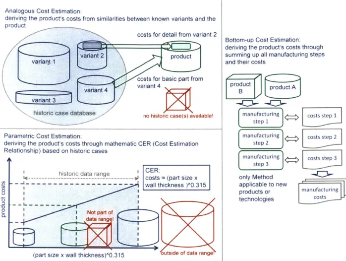
Curran presents a taxonomy for classifying different methods for cost estimation tools into three categories: analogous, parametric, and bottom-up. Hueber et al [2] follow Curran in classifying cost modeling approaches into bottom-up, parametric and analogous. Weustink [1 3] by contrast, makes the point that parametric and analogous just represent the same approach to different fidelity levels: parametric methods are a mathematical fonnalization of analogous methods.

Figure 7 contrasts the different cost modeling approaches as categorized by Hueber et al., based on Curran et al., into analogous, parametric and bottom-up. It can be seen in the figure that analogous and parametric approaches both build on existing product cost information. The analogous methods are some of the easiest to implement and naturally what many designers default to. In a sense, the parametric method is just a mathematical formalization of the analogous method: it simply interpolates between existing products based on important features of the design to arrive at an estimate.

Analogous Cost Estimation:

deriving the product's costs from similarities between known variants and the product

costs for detail from variant 2

variant 2 \product variant 1

costs for basic part from

4vari ant 4

s ca ase no historic case(s) available!

Parametric Cost Estimation:

deriving the product's costs through mathematic

Relationship) based on historic cases CER (Cost Estimation

Ihistoric data range CR

... ... costs - (part size x

n - .i. - - - - wa hikss).35

wall thickness )A 0.315

0

2 1 Not part of

_L rangen odata

(part size x wall thickness)AO.315 outside ofdata range.

Bottom-up Cost Estimation: deriving the product's costs through summing up all manufacturing steps and their costs

roduct

manufacturing A _tepi

manufacturing

manufacturing _{costs step 2} step 2

manufacturing _{costs step 3}

step 3

only Method

applicable to new

r

products or manufacturing

technologies costs

Figure 7. Schematic description of top-down (left) and bottom-up cost estimation approaches. Reproduced from [2]

Whereas the top-down approach of the DAPCA system is easy to apply at the beginning of the design process, when basic extrinsic data about the aircraft design are available, the bottoms-up approach of COSTADE requires specific design details about each individual part in order to estimate the total construction cost. The advantage of the bottom-up approach is that specific cost drivers can be identified and tied back to specific components. Together, the approaches established by DAPCA IV and COSTADE and the models they provide have been implemented within a number of software tools for manufacturing cost forecasting.

/

Figure 8. Classification of estimation models [2]. The division into parametric and suggested by Curran [11], but rejected by Weustink [13], who summarizes parametric models as variant-based (and bottom-up as generative.)

analogous was and analogous

Figure 9 weighs the relative merits of the different approaches according to Curran et al. and Hueber et al., which this thesis will expand upon.

Bottom-up

Analogous

Method

Method

ALPHA

Parametric

Analogous cost estimation

Parametric cost estimation

Bottom-up cost estimation

-Cause and effect understood

-Quick and easily applied

-Based on actual historical data

-Accurate for minor deviations from analog

-Easiest to implement

-Developed CERs are excellent tools for "what-if"analysis

-Non-technical experts can apply method, no reliance on opinion

- 'Statistical' uncertainty of the forecast is generated

" Allows scope for quantifying risk

" Cause and effect understood

-Intuitive and defensible

-Very detailed estimate

- Provides insight into major cost contributors

" Miscalculation of an individual element does not compromise entire estimation

Figure 9. Summary of advantages and disadvantages of the three main cost estimation methods, summarized by Hueber [2] largely from [1 1]

Table 2. Summary of available cost estimation tools

Name Classification Release Availability Scope Summary

Initial/ Latest

DAPCA[7], Top-down 1967/ Public Lifecycle Regression fits to data from

[14] _{previous aircraft programs.}

ACCEM [8] Bottom-up 1976 Public Manufacturing Cost estimating relationships derived from time and motion studies of manufacturing processes.

COSTADE Bottom-up 1996 Public Manufacturing Takes geometries and process

[10]

Processes _{selection as inputs. Bottoms-up} approach looks at the fabrication of every component.

SEER-MFG Top-down and Commercial Manufacturing An easy, off the shelf tool but

[15] bottom-up License the models are not available so solutions can be opaque

Method Advantages Disadvantages

- Appropriate baseline must exist

- Identifying the appropriate analog can be difficult

- Substantial, detailed data are required

- Requires expert knowledge/judgement for adjust-ment factors

-Can be difficult to develop

- Factors might be associative but not causative (i.e. lack of direct cause-and-effect relationships

-Relationship might not be easily understandable

-Selection and adjustment of raw data and devel-opment of equations, statistical findings conclu-sions must all be documented for validation

-Extrapolation of existing data to forecast the future, which include radical technological changes, might not be properly forecast

- Loses predictive credibility outside its relevant data range

- Difficult to develop and Implement Substantial, detailed expert data are required

- Requires expert knowledge

" Significant effort (time and money) required to create an estimation

- Does not provide good Insight Into cost drivers

- Estimate must be "built-up" for each alternative scenario; not responsive for "what-if"analysis

2.2.

_{Conceptual Aircraft Design: Different Approaches}

The challenge of aircraft design is as complex as the machines it produces; modern aircraft like the Boeing 787 have millions of parts2

, each conceived to perform a certain role and tested, first in a computer then in real life, to assure that it can perfectly perform its role. Before reaching detailed design of these parts, the aircraft goes through conceptual design where different design concepts are proposed and evaluated to select the designs which will be fleshed-out in the detailed design phase [16]. Raymer provides specific guidance to the designer about the order in which the designer should iterate through solving design equations in order to find an aircraft design which feasibly (but not optimally) meets the design criteria.[1 6] During the conceptual design phase, designers often will use optimization tools to find the best designs and characterize trade-offs between design decisions. Multidisciplinary design optimization (MDO) is a method to integrate models and simulations of candidate designs and is often used as an optimization tool during conceptual design.

Figure 10 shows the interface of AVID ACS software used to model the physics of an aircraft in the conceptual design phase.

I I OMO~ 9 n W "30 . W~RA O 14 T.. 4

~

00 -..5~-.2 .. 5s, c ,4. S . l Zty Sinllzd:33 *

~ ~

~

f 3 1lM.W u

if 2 A WEm-2 ..KSE.6. IP% 1N4 , rums R.. 2%.s 35GO.O1, T P.0,

87 N6@@.6,AtA.4. . oc oo6T.oFog6.0oo

MAOV4ftuI1' Le..0..0 SEWu~~o

9 PS NFI~OS- fiCA.020 51wT-2 0 luS I

= -Z. m. PSM4.o wu 0. ral 60 3s.

WDOW4 S(.0 gri&Ars

Figure~~~OOTA 10Notaeitraeof VIDAScneta icrfemtydsg.

Modem CAD~~~~~IM tool from Siemen [1] and Dasal S e [1]icuebit-nwrfoso

exera ad-nWhtalwtedsgeNog _{rmpr esg oFAsmlto oeaut tutrlo}

aeoyai pefomace s wel asT anuatrn:rcs eeto n iuainhscnutmtl

leattosfrdsgigtelyuoftefcoytbulthprdc.Tiinerto _isrltvlnw

and~

~

O alow for 7 reeecst 0h*rgnldsg ob aiy anandtruhteetr einpoes

Examples"L nclude _{, Simuayt Composites Modee o Sldokso o frAausCB ISAYwt} ANSYS ProO ENIER or CATIA Anglp Lamnat Tol for f OoDdwrk or for ANY0 and0

CATIA v5/6 Copsie Deig (ht:/w6iiaeg newsde/p6ao6-fr-cmpos esanalsisand simulatiCo. g~r User can' deine ie usn5ondr0uve na ndryn9srae0hetosprvd h

connectivityWq0.6,O bewe thUifrnteautonses0u silrl o h eine4opoid nust

improve the design. These CAD tools, advanced as they may be, support only design development in one direction from aircraft configuration to manufacturing planning.

-

--.. , , --.a

. men1

Irv:

Figure 11. Interactive Ply Table in Grid Design in CATIA Composites from Dassault Systemes [18]

Mikrosam, a manufacturer of automated fiber placement machines used to produce composite aircraft structures, also released a software package that aircraft designers can use to plan and simulate the process. "MikroPlace provides a sophisticated environment for the composite part designer to be able to create composite structures using automated fiber and tape placement (AFP/ATL) techniques, and at the end, to generate the actual program to be executed on AFP or ATL machines. The part designer can perform most of the necessary steps in developing an advanced composite part right in the MikroPlace environment, by being able to draw or import the part's tool, create ply laminates from numerous strategies, export the composite for analysis to popular Finite Element Analysis (FEA) software packages, analyze and fix

ID ~

-Figure

2.3.

_{Composite Aerospace Production Systems}

Modem airframes, be they composite or traditional metallic construction, are assembled from large modules which are in-turn assembled from smaller submodules. Figure 13 shows how a Boeing 787 is assembled from myriad different sub-assemblies made by Boeing and Boeing's partners around the world.

SOMW

Wing tips

Fixed trading edge

Nagoya, Japarn

ol,"asalvi .;

Moveable trailing edge

Melbourne. Australia (Boeing)

Flap suppodt fabbngs

i luaSouh KoPral('AL-AS I

Naaegts

Wing C hot$ Vtta,

%agoya. Japan Cadoma. USA Mtsutsto} (Goo (ich)

Midyfouad %*aws&

Nagoya, Japatn (Ilawasal

Fotward fosafag. Wdaictx. xansos WSA

Cargo access doors

LiOPin .SwOden (SROPh'

S Center fatag" Grottaglie. Italy

Wingibody fairing

L~anding gear doors

Center wing ban .cisa0

Nagoya. Japan (Fuoi

Passenger entry doors

Tolouse France (Latrcore'

A Main anding g(awr s l WON Nagoya. Javan l(awasalul Gkuxxestr. UK tKMeSser-O0Wty)

Evendale, O"o, USA fGEl

Derby U11. (Rolls Royce)

Fixed ad noveable

adi edge

Tulsa Oklahoma USA iSpoiif

Figure 13. The Boeing 787 is assembled from many different large sub-assemblies manufactured by Boeing and its partners from around the world.4

Whereas Boeing's 787 fuselage sections are produced as single-piece "barrels", Airbus' A350 sections are produced as separate pieces that are later assembled into a barrel, as shown in Figure 14.

Aft fuselage usano. South Koea (IIAL-ASD) Nortrontal Foggia. saty Atenait

Crow.n SDUMa

" Oarmotu To$ LsW. han" Wd OMPs40wd Snserfn O6ndS 1*-SW

" TWS* Af~ Wd RTM FiWmss CO-*do S -0

pe compesd and cued to form the lt e Tha r& fber Tere ome s &in genealy w f : dswde

*~TOM T0 P,"~ MU ftrpe W&P~ 0 Skin~

~p~Uw

Figure14.A fuslag s-sembly showin it assmbl from ajor copoit om ponnt and the'

plies andresinare W compressd adecred o for tWihe uliae at

Thge aw cAo fiblae muate comesigra itwo forems:y froadgoodsr(sheetsior wideorolls oarndh

fiber) and spools of tape or tow. Broadgoods and tapes can be comprised of fibers in a single direction (called unidirectional or UD) where the fibers can be oriented across the axis of the tape or along the axis of the tape. Broadgoods and tapes are also made from woven fibers as well. The material width distinguishes tapes from broadgoods; tapes are generally narrower than 450mm.6 Tows are spools of unidirectional fibers along the axis of the tow and are not woven. Usually tows are narrower and contain fewer fibers than tape. Large broadgoods can be cut down into specific shapes and placed (by hand or machine) to molds. Broadgoods can be woven in a number of patterns to obtain different strength properties. Tape products have high strength in the fiber direction. They are stacked up in different orientations ("stacking sequences") to increase overall stability. The layup is a serial process.

Tapes and tows are usually placed by machine onto a mold or tool. These automated pieces of equipment are often known as automated tape laying (ATL) or automatedfiber placement (AFP) machines.

Tapes are often better suited for large, nearly flat parts (like wing skins) whereas tows are better to layup

5 source: http://dfat.gov.au/about-us/publications/trade-investment/trade-at-a-glance/trade-at-a-glance-2014/Pages/performance-08-global-value-chains.aspx

I4

on more contoured surfaces (like fuselages or wing spars). In many cases, the ATL or AFP machine can simultaneously deposit multiple tapes or tows onto the composite tool at a single time.

If the raw materials come pre-impregnated with resin, the production process is known asprepreg. The raw materials must be stored in freezers prior to layup in order to prevent premature curing. After layup, parts are prepared for curing. Most of the resins in commercial production are cured by heating. Some parts are cured in an autoclave which, in addition to heating the part, increases the ambient pressure around the part (like a giant pressure cooker) to compact the plies together and create a stronger part. Once the structure is cured, holes can be drilled (thousands of holes per aircraft), floors and interior can be mounted, etc.

Of course, errors or defects can occur in any of these processes along the way. Correcting such defects has comparatively different effects on overall system performance between metallic and composite construction techniques. With metallic construction, the defect can usually be isolated and work can continue on other components of the assembly. With composite materials where fabrication is highly serial and additive, errors cannot be easily isolated and correcting a defect often interrupts all other work on the part.

In either case, taking time to correct defects add variance to processing times. Timing variance has a more negative impact on the performance of composite production systems than the same variance would have in a metallic production system. The more serial nature of composite fabrication makes it difficult to continue work while addressing a defect. Variation plays a more significant role in composite fabrication than it does when building airframes out of aluminum.

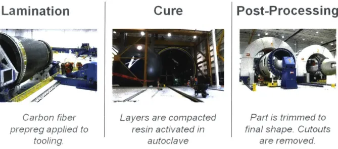
By way of an example, the primary processes for fabricating a fuselage are shown in Figure 15. The fabrication process begins with lamination where the preimpregnated, carbon fiber tows are laid up on the tooling mandrel that forms the inside of the fuselage (or the inner mold line). An automated fiber placement machine (AFP) is used to lay up the composite tows. This machine makes multiple passes for each layer and all of the layers together form a stack. After all of the layers of carbon fiber have been applied, the stack and the tool are prepped and transferred to the autoclave. The autoclave executes a pre-programmed curing recipe that defines required temperature and pressure in time. An example recipe is shown in Figure 16. The high internal pressure in the autoclave compacts all of the layers and the elevated temperature cures the epoxy resin impregnated in the carbon fibers. After curing, the hardened part is removed from the autoclave and placed on a machine for post-processing to make any cutouts and trim the part into its final shape.

Lamination

Carbon fiber

prepreg applied to

tooling.

Cure

Layers are compacted

resin activated in

autoclave

Post-Processing

Part

I

rimed t::

final shape. Cutouts

are removed.

Figure 15. Depiction of the three primary processes in fabricating a composite fuselage.

r4

12OW

40W_:

Mr-Iv t Z2ir r 41 tu 5 r t

Figure 16. A process diagram for a typical autoclave curing cycle for a small composite part. The chart shows the nature of the process beginning with a temperature ramp up to the dwell temperature and pulling a vacuum on the part. The temperature is again ramped up from the dwell temperature to the curing temperature as the atmospheric pressure is increased in the autoclave. As the cure completes, the temperature is returned to ambient, the vacuum on the part is relieved and the atmospheric overpressure in the chamber is released.

rvww~se 61

Ows~n v IU rha

Time

2.4.

Toward Manufacturing Cost Estimation in

Conceptual Aircraft Design

The previous sections have highlighted different approaches to (a) predict the production cost or life cycle cost of an aircraft and (b) facilitate conceptual aircraft design. It was also argued that the important design decisions are made early on and the majority of costs are committed early on in the design process. Thus, there exists a need for cost estimation tools in conceptual aircraft design.

Tools exist (NX and CATIA) for evaluating the structural performance and manufacturability of components during design. They rely on the designer to change the inputs in order to improve design. Multidisciplinary optimization (MDO) seeks to close the loop around the design process to automatically alter the design and evaluate its performance in order to improve given metrics (usually weight).

Usually the performance of the design is evaluated against structural simulations (FEA), aerodynamic simulations (CFD), and other assessments of flight characteristics. Often the objective of the MDO is to minimize the weight of the aircraft. Usually the assumption is that minimizing the weight will minimize the manufacturing and operating costs of the aircraft.

Work done by Karen Willcox and her students at MIT [20]-[22] add models for cost or value to the traditional MDO framework to allow more explicit maximization of value or minimization of cost. In these cases, a weight-based cost estimating relationship (CER) is used to estimate manufacturing cost. Thus, from a manufacturing cost standpoint, these are top-down methods.

Other authors employ bottom-up methods for estimating manufacturing costs. Figure xx below shows the approach by Hueber et al. [2] to combine cost estimation with conceptual design in this MDO framework. They call their tool "ALPHA."

Designi

Weight

4

Feat

Weight Manufact.

Manufact..-Penalty _{Cost Cost Model}

H

E

DoC Process

Direct

Operating

Co ts _Adadule

Objective Function Mdl

e Constraints

Figure 17. Framework for design and manufacturing co-optimiz ures KB Expert PAM) IKnowledgei Finite Failure Element Prediction Analysis

ation outlined by Hueber et al. [2]

Mavris et al. have created an MDO framework they call "Manufacturing Influenced Design (MInD)" shown in Figure 18. [23]-[25] There has been significant follow-on work to include an interface for design space exploration (MInD SET) and a version with integration to Simio design and simulation tools (MInD SET PRO). In addition to the traditional structural and aerodynamic simulations, MInD includes calls to SEER-MFG to obtain manufacturing cost estimates to help drive to a cost-minimizing design. The MInD tool also includes a dashboard to allow designers to evaluate trade-studies to see how different design changes influence the cost of the aircraft Figure 20. The MInD tool takes, as input, a concept airframe design and can provide comparative manufacturing trade-studies between the candidate designs.

Recent work from Georgia Tech has integrated factory dynamic simulation tools with concept-phase models [23], [26]. The "Manufacturing Influenced Design (MInD)" environment takes aircraft geometries as input, evaluates structural and aerodynamic performance of the components, predicts process times using off-the-shelf software (SEER-MFG by Galorath), and discrete event simulations of factory dynamics and supply chain to ultimately predict the production cost of the input design. However, since the MInD approach implicitly relies on Monte Carlo methods (see Chapter 4.1 of this thesis), determining the sensitivities between variables is difficult. Furthermore, the approach thus far implemented, requires a design of an aircraft and a supply chain as inputs. Therefore, it is difficult to quickly investigate many different concepts for the production system or to rapidly explore various design trade-offs, known as the "tradespace."

As Figure 18 and Figure 19 show, MInD and MInD PRO essentially help the designer draw a "black box" around other software packages, such as SEER-MFG, which in itself acts like a "black box".[27] The

great advantage is that these are tools many engineers are familiar with. Obvious limitations are: very slow execution speed due to the great number of numerical operations that have to be performed, limited flexibility for use with breakthrough innovations in materials processing not captured by the proprietary software, and limited scientific merit due to the covet proprietary nature of the utilized software.

1. Design Detailed 2. Generate Detailed Parametric System Geometry Data

6. Abstract Preliminary Level

RSEs from Detailed Data 5. Run Design of Experiments

"Pm peen COW 7. nr

I=

s T rdM m _ThtW MmW 4~m _L~ WOW Was" to 40 Wa

7. Incorporate RSEs Into MinC

Trade-Off Tool

3.S

Sc

etup Performance, Manuf. Cost, heduling, & Cash Flow Models

4. Integrate Parametric Model

Emp

Repeatapproachfor various designs, materials,

and processes to

incorporate RSEs into

MinD Trade-off Tool.

Figure 18. The Manufacturing Influenced Design (MInD) tool from Dimitri Mavris et al. from Georgia Tech. [23]

Parametnc Dstailed Fabrication Cost Model

PrFEMetri pi Structw/

~by

Part + Assembly

M

EM s ai0M u c ri - Cost Modelem

MSI

asr

Data Tranlator

I

SEER

Manufacturing Costs

J

RDT&E and O&S Cost

E

P

aPlanning Chain

(FLOPS)

_

Optimization

optimization

Performance RDT&E / Prod Cycle Supplier & Data O&S Costs Time, Tooling, Logistics

& Capital Cost Cost

MInDSET GUI

Risk Surrogates

A st E om Varables

Key Economic Variables

Figure 19. The software components of the MInD multidisciplinary model. Dr. Dimitri Mavris' group has been working on at Georgia Tech.

aw" mo I.rm _ UUnecdDso I"dcio 0kiwK

rj

I-r

i1

4WA-*b 'a tobH~

=

rv1=

Figure 20. Dashboard interface to the Georgia Tech MiND SET PRO tool.7

7 source: https://www.asdl.gatech.edu/AdvancedConcepts.html

Design Variable

14-3.

GEOMETRIC PROGRAMMING:

F

RAMEWORK

3.1. Background

This section offers an introduction to the Geometric Programming (GP) form of optimization. The primary source for the background information in this section comes from Boyd et al. "Tutorial on Geometric Programming" [28] and is partially summarized in this thesis for completeness. Geometric programming can solve non-linear optimization problems extremely quickly, with the caveat that the objective function and constraints can be represented in a certain mathematical form.

Geometric programming was originally introduced in the 1960s. It has only been with the recent introduction of efficient solvers that the full power of the GP form is beginning to find use. Geometric programming has helped to solve design problems in several engineering disciplines including aerospace

[29], water utility control [30], and communications and electronics [31], among many others.

Recent work from MIT and Berkley has produced new methods for modeling and optimization during the conceptual design phase using Geometric Programming (GP) [20]. Geometric Programs are particularly well-suited for aircraft design optimization because of their ability to handle nonlinear constraints.

3.1.1.

GP Formulation

A geometric program is a convex, non-linear, constrained optimization program of the form

minimize fo(:)

subjectto fi(k) : 1, i =1, ... , p

giG) = 1, i=1.m (

Xi > 0, VXi IE

where : is the vector of decision variables

where g(Y) is a monomial' of the form

g( ) = CXax11 ₂a2 ... Xa",xn c > 0

and where

f(z)

is a posynomial, a positive sum of monomials, and has the form

K

f )= CGx₁ X ... ,

k=1

Ck > 0 Vk,

An example of a monomial as in (3) could be

3

7TX'X₂

and an example of a posynomial as in (4):

2x1x2 + x-0.5 6

Boyd also notes that a posynomial that is less than or equal to a monomial,

CkX alkX azk ... Xank < CX1,x2 ... Xan

(5 )

Ck 1 X2 n'

~

1 2 an(5 k=1

is a valid constraint for a geometric program. By dividing the posynomial on the left hand side by the monomial on the right hand side, one obtains a posynomial inequality in the canonical form shown in (1). This thesis frequently presents posynomial inequalities in the form of (5).

Developing a "GP model" means finding exact or approximate monomial or posynomial constraints to capture the behavior of the underlying problem. Boyd et al., Hoburg, and others show that many, fundamental physical laws, like F = ma, or well-known approximations can be directly relaxed into the form the GP constraints require. Despite the nonlinearities, constraints of this form are very fast to solve

8 Note this is different from the normal, algebraic definition of a monomial. This work will refer to this GP

definition of a monomial.

(3)

with convex optimization methods. This allows for rapid exploration of the aircraft trade-space and gives a wealth of sensitivity data in addition to an optimal solution.

For the models in the context of this thesis, there are three types of variables which are discussed: free and fixed decision variables and parameters. Parameters are values which the user may want to vary but are not part of the geometric program itself. Parameters appear as constants in the GP constraints.

There are many decision variables throughout the GP. Decision variables for which a value is fixed prior to optimization are termed "fixed variables" whereas decision variables that are not fixed and are free to be optimized are appropriately termed "free variable." Not all combinations of free and fixed variables will produce a feasible GP. If there are free variables which are not bounded, the GP is said to be "dual infeasible" and cannot be solved. On the other hand, a GP is "primal infeasible" if there is no solution which can simultaneously satisfy all constraints.

This thesis distinguishes "parameters" from "fixed variables." Though both are inputs to a particular problem, "fixed variables" could be turned into "free variables" and, provided the GP is still feasible, optimized. Variables, both fixed and free, form valid GP constraints. Parameters, on the other hand, must be provided as inputs in order for the problem to be a valid GP. Consider the constraint

1 3x" + x2

The constraint is valid as a GP with x1, x2 as free or fixed variables. However, a,

fl

must be "parameters"

because they cannot be decision variables in a GP.

Selecting which variables should be free and which should be fixed to properly bound all of the free variables is an important step to contextualize the models to answer a specific question. For example, using the models to predict how much a new airplane with certain performance will cost requires a different context than what the best performing aircraft for a particular budget constraint could be.

Inputs to the model are values for all the parameters and any variables to be fixed. Outputs from the model are the value of the objective function at optimality (often a cost in dollars), the optimal values for the free variables and sensitivities to fixed variables.

3.1.2.

Solving GPs

and each side of each constraint are taken. Since xi > 0 as defined in (2), this logarithm is always defined. Note that the right-hand-side of the constraints, both monomial equalities and posynomial inequalities, are replaced with log(1) = 0. After transformation, the optimization takes on the form

minimize logfo(e-)

subject to log

fi(ey)

0, i = 1, .. , p (6)

log g (e) =0, i= 1, .m

where

Y

is a vector (y1, Y2,..., yn) and thus e- is a vector formed by component-wise exponentiation

e = (es', eY2, ... , en) ₍₇₎

The trick here, as Boyd et al. point out, is that the original, untransformed GP is non-convex but that its log-transformed problem is convex. This assumption of the form of geometric programs guarantees that they are "log-convex" (by assumption) and are thus transformed to be solved as convex optimization problems. This assumption holds because a monomial with positive terms is log-convex. A posynomial, which is a positive sum of monomials, is also therefore log-convex. The only other assumption of the form of the model is that the variables and coefficients are positivite.

To demonstrate this transformation, consider a simple monomial function:

3xO5 (8)

Substituting x = ey and taking the log-transformed version of (8) is

log 3(ey)0_.5 _{= log 3 + log(e}0_{osy) = log 3 + 0.5y}

(9)

Figure 21 shows plots of the untransformed function (a) and the log-transformed function (b). The original function (8) is concave (and thus non-convex) but the transformed function (9) is linear and affine (which is convex.)