Computational modeling of simultaneously recorded scalp and depth EEG signals

HAL Id: hal-00331549

https://hal.archives-ouvertes.fr/hal-00331549

Submitted on 17 Oct 2008

HAL is a multi-disciplinary open access

archive for the deposit and dissemination of

sci-entific research documents, whether they are

pub-lished or not. The documents may come from

teaching and research institutions in France or

abroad, or from public or private research centers.

L’archive ouverte pluridisciplinaire HAL, est

destinée au dépôt et à la diffusion de documents

scientifiques de niveau recherche, publiés ou non,

émanant des établissements d’enseignement et de

recherche français ou étrangers, des laboratoires

publics ou privés.

Computational modeling of simultaneously recorded

scalp and depth EEG signals

Delphine Cosandier-Rimélé, Isabelle Merlet, Jean-Michel Badier, Patrick

Chauvel, Fabrice Wendling

To cite this version:

Delphine Cosandier-Rimélé, Isabelle Merlet, Jean-Michel Badier, Patrick Chauvel, Fabrice Wendling.

Computational modeling of simultaneously recorded scalp and depth EEG signals. Deuxième

con-férence française de Neurosciences Computationnelles, ”Neurocomp08”, Oct 2008, Marseille, France.

�hal-00331549�

COMPUTATIONAL MODELING OF SIMULTANEOUSLY RECORDED

SCALP AND DEPTH EEG SIGNALS: INSIGHTS INTO THE

INTERPRETATION OF INTERICTAL EPILEPTIC ACTIVITY

D. Cosandier-Rimélé1,2_{, I. Merlet}1,2_{, J.M. Badier}3,4_{, P. Chauvel}3,4 _{, F. Wendling}1,2 1 _{INSERM, U642, Rennes, F-35000, France}

2 _{Université de Rennes 1, LTSI, Rennes, F-35000, France} 3 _{INSERM, U751, Marseille, F-13000, France}

4 _{Université d’Aix Marseille 2, LNN, Marseille, F-13000, France}

ABSTRACT

In epileptic patients candidate to surgery, the interpretation of electrophysiological signals recorded non-invasively (scalp EEG) and invasively (depth EEG) is a difficult but central question. Indeed, the localization of the epileptogenic zone, the determination of its organization and the definition of subsequent therapeutic strategy are still largely based on the analysis of electrophysiological data. This issue is addressed in the present work through a realistic modeling of both scalp and depth EEG signals. The model is based on an anatomically and physiologically relevant description of the neuronal sources of brain electrical activity that combines a distributed dipole source model with a model of coupled neuronal populations. EEG signals are then simulated by solving the so-called forward problem in the head volume conductor, simultaneously on scalp and depth electrodes. The model allows for the study of the influence, on simulated EEG signals, of source-related parameters (spatial extent, synchronization) leading to the generation of transient epileptic activity (interictal spikes). More generally, this modeling approach helps in the understanding of the relationship between the properties of signals collected by electrodes (scalp and depth) and the underlying spatio-temporal organization of the neuronal sources.

KEY WORDS

Epilepsy, EEG, scalp, depth, modeling, simulation.

1. Introduction

In patients with drug-resistant partial epilepsy, the identification of brain areas responsible for the generation of epileptic activity is required to define subsequent surgical strategy aimed at suppressing seizures. Among the many investigation methods performed during presurgical evaluation, scalp EEG and depth EEG play a key role as they both provide real-time markers of brain electrical activity, in the form of time-series signals with excellent temporal resolution. Scalp EEG and depth EEG are two different modalities which provide information at two different spatial scales. In scalp EEG, a set of electrodes positioned on the scalp is used to record the global brain activity. In depth EEG, multiple contact electrodes directly implanted into target brain structures are used to record the local field activity. In both modalities, the recorded signals reflect the epileptic activity generated

by epileptogenic networks either during ictal (seizure) or interictal (outside seizures) periods. Prior to surgery, the thorough interpretation of these electrophysiological signals is an essential step that must lead to the localization of epileptogenic networks and to the determination of their topology.

However, the interpretation of EEG data remains a difficult problem for two reasons, at least. First, the generation of brain electrical activity is a highly complex process resulting from various coupled nonlinear mechanisms lying at subcellular, cellular and network levels. Second, the relationship between the activity generated at the level of neuronal networks and the signals actually observed at the level of electrodes is not straightforward: scalp and depth EEG signals correspond to the projection, onto spatially distributed sensors, of specific neuronal mechanisms (mainly post-synaptic) taking place into interconnected populations of neurons, themselves distributed on the folded neocortical surface.

In this paper, we propose a computational modeling approach aimed at tackling the complex relationships between neuronal sources at the origin of brain activity and recorded EEG signals [1,2]. This approach is based on the realistic representation of the sources, as well as the computation of the electrical potentials recorded by electrodes (forward problem). The model is then used to study the influence of source-related parameters (spatial extent, synchronization level) on the signals simulated in both modalities.

2. Spatio-temporal extended source model

and generation of EEG signals

The proposed approach is based on i) a spatio-temporal representation of the neuronal sources of activity, and ii) the computation of the EEG signals induced on scalp and depth electrodes.

2.1 Spatio-temporal extended source model

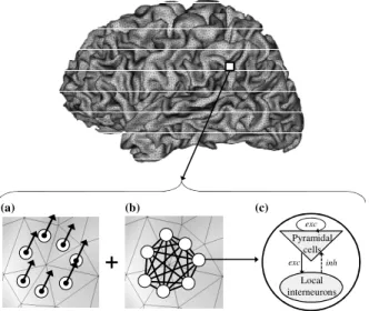
As illustrated in Fig. 1, the developed source model combines a biophysical dipole layer source model (Fig.1-a) with a biomathematical model of coupled neuronal populations (Figs.1-b and 1-c). The former accounts for the geometrical properties of the sources whereas the latter generates realistic time-courses for the activity of current dipoles associated to neuronal populations. In the current version of the model, the sources of EEG are restricted to the pyramidal neurons

of the neocortex, i.e. subcortical structures are not taken into account. Moreover, it is assumed that the neocortex is organized as a network of neuronal populations. The current dipole associated to each neocortical neuronal population provides its electrical contribution. It is characterized by three parameters: its location, its orientation and its intensity. Constrained dipole locations and orientations were obtained from a realistic mesh of the neocortical surface (Fig. 1) built from the segmentation of 3D MRI data (BrainVISA package (http://brainvisa.info/)) [3]. The high resolution of the mesh ensured an accurate description of the circumvolutions of the neocortical surface (about 80000 triangles per hemisphere). The average surface of each triangle, corresponding to a distinct population of neurons, was equal to 1 mm². One dipole was located at the barycenter of each triangle and was oriented normally to its surface.

Fig. 1: The model starts from a realistic mesh of the neocortical surface obtained from MRI data. Description of spatial and temporal features of the neuronal sources was achieved by combining (a) a distributed dipole source model with (b) a model of coupled neuronal populations. (c) Each neuronal population contains two subsets of neurons: the main pyramidal cells and the local interneurons. Pyramidal cells receive excitatory input (exc) from other pyramidal cells (collateral excitation) and inhibitory input (inh) from inter-neurons. These latter cells receive excitatory input only from pyramidal cells.

Each dipole intensity was obtained by multiplying the corresponding triangle surface by the cortical dipole moment surface density (time-invariant). The result was then weighted by a time-varying coefficient that reflects the time-course of the activity of the neuronal population associated to the triangle. This coefficient is provided by the output of a neurophysiologically relevant model, able to produce signals (local field potentials) from networks of coupled neuronal populations [4].

In this model, a set of interconnected populations of neurons is considered. As illustrated in Fig. 1-c, each neuronal population is composed of two subsets of neurons: the main pyramidal cells and the local interneurons. Both subsets mutually interact through excitatory and inhibitory feedback. In each subset, input-output relations are specified by two functions, often referred to as the “pulse-to-wave function” and the “wave-to-pulse function” in the literature. The

former is a linear transfer function that changes presynaptic information (i.e. the average density of afferent action potentials) into postsynaptic information (i.e. an average excitatory or inhibitory postsynaptic potential). The latter is a static nonlinear function that relates the average postsynaptic potential of the subset to an average density of action potentials fired by the neurons. Furthermore, the connection from a population to another is characterized by two parameters, defining the degree of coupling and the time-delay associated to the connection. An appropriate setting of these parameters allows for building specific networks inside which neuronal populations can be unidirectionnally and/or bidirectionnally coupled (see [4] for details). In this model, neuronal populations can be rendered as “epileptic” by adjusting some parameters (excitatory and inhibitory gains in feedback loops, degree and direction of coupling between interconnected populations). Therefore, such settings can be used to simulate the time-courses of “focal epileptic sources” (i.e. neocortical patches generating interictal spikes) with surrounding normal background activity.

2.2 Generation of EEG signals

Electrical potentials induced on scalp and depth electrodes were computed by solving the so-called EEG

forward problem, i.e. by computing the electrical

potential generated by a given source in the brain. In order to solve the forward problem, a model for the head volume conductor is required. This model accounts for the geometrical and physical properties of the different head tissues (shape and conductivity). For depth EEG signals, the head was assimilated to a set of three concentric homogeneous spheres representing the brain, the skull and the scalp. The conductivity of the skull was assumed to be 40 times lower than that of the brain and scalp, which were set to a same value of 0.33 S/m [5]. In the spherical head model, the forward calculations can be performed at any point in the head volume using an analytical expression (see [1] for details).

For scalp EEG signals, a more realistic head model was used, as the locations of scalp electrodes strongly depend on the head shape. This model consisted in three nested homogeneous compartments (brain, skull and scalp). Surface boundaries between the three tissues were extracted from 3D MRI data, using the ASATM software (ANT, Netherlands). Compared to the source model, a lower mesh resolution was used to approximate the shape of volume conductors (2440 triangles per boundary). In the realistic head model, the forward calculations must be performed using a numerical method. In this study, we used the isolated problem approach of the boundary element method [6].

3. Parametric study

The EEG generation model was used to study the influence of some source-related parameters, on simulated scalp and depth EEG signals. To proceed, we defined three simulation scenarios, each one addressing the specific influence of one parameter. These scenarios were motivated by recurring questions in the context of

+

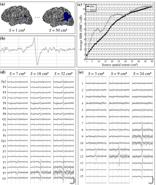
EEG analysis in epileptic patients: 1) the spatial extent of a focal source of epileptic activity, 2) the location of this source and 3) the synchronization degree between neuronal populations within this source. In this paper, we will focus on the spatial extent (scenario 1) and on the synchronization degree (scenario 2) of an epileptic patch positioned in the left temporo-parieto-occipital region (Fig. 2-a). For both scenarios, scalp and depth EEG signals were simulated simultaneously. Scalp EEG signals were computed over 63 electrodes distributed on the scalp according to the standard 10-10 electrode system. Depth EEG signals were computed at the 15 contacts along an intracerebral electrode, orthogonally implanted in the center of the epileptic patch.

The influence of the aforementioned parameters on signals simulated in both modalities was analyzed qualitatively and quantitatively using a criterion based on the spike-to-background ratio (SBR), defined for each sensor as the ratio between the average power of the spike and the average power of the background activity that precedes and follows the spike:

, i = 1,…,M where xi(t) is the electrical potential recorded at discrete time t, at the ith sensor (i=1,…,M), s ( b) and ns (nb) denote for the time support and the number of time samples for the spike (the background) respectively. For both scalp and depth EEG signals, SBR values were then averaged over the M sensors, leading to a “global” criterion (denoted by an asterisk):

! " #$

4. Results

4.1 Scenario 1: spatial extent of the source

We varied the spatial extent of the considered epileptic patch (fixed location) from 1 cm² to 50 cm² (Fig. 2-a). The same time-course was associated to all dipoles within this patch. It corresponded to an epileptic spike (Fig. 2-b) generated by the neuronal population model for an increased excitation-related parameter. The time-course assigned to all other dipoles (outside this patch) corresponded to different realizations of the background activity obtained for a “standard” excitation value in the population model.

Fig. 2-c shows the evolution of the SBR* _{quantity with}

respect to the patch surface, for scalp and depth EEG signals simulated over the same time epoch. Three main remarks can be made on these results. First, for both modalities, the SBR* _{increased as the surface of the}

epileptic patch increased. The obtained curves followed a logarithmic shape, the SBR* _{increase being less}

pronounced for larger patch surfaces. Second, the SBR*

curve was found to be smoother for scalp EEG, compared to depth EEG. Particularly, in this second modality, the curve showed several local minima. Third, for a patch surface inferior to about 30 cm², the

SBR* _{values obtained from simulated depth EEG were}

higher than those obtained for simulated scalp EEG. In particular, the characteristic value of SBR* _{= 3dB (i.e}

spike amplitude equal 1.5 times the amplitude of the surrounding background activity) was obtained for a patch surface of 3 cm² in the case of depth EEG signals, and for a patch surface more than twice as large (7 cm²) in the case of scalp EEG signals.

The simulated scalp and depth EEG signals for three specific SBR* _{values (3, 6 and 9 dB) are illustrated on}

Figs. 2-d and 2-e. As depicted from Fig. 2-c, these values were obtained for S = 7, 18 and 32 cm² (scalp), and for S = 3, 9 and 24 cm² (depth). The visual analysis of scalp EEG signals showed that for S = 7 cm², spikes were observed on electrodes P7 and T7 “facing” the epileptic patch. As the patch surface increased (S = 18 cm²), the spike amplitude was higher on these electrodes (as expected) and a concomitant spike of inverse polarity was clearly visible on parieto-central (Cz, Pz) and contralateral electrodes (F4, C4, T8, P4, P8). For a surface of 32 cm², the spike was visible on almost all scalp electrodes. Simulated depth EEG signals are displayed in Fig. 2-e. For a 3 cm² patch, the spike appears on the most external sensors (11-15) with a maximum on contact 12. When S = 9 cm², the amplitude of the spike increased on contacts 11 to 15 with still a maximum on contact 12. A small amplitude spike could also be detected on several deeper contacts (7-10). For a 24 cm² patch, the spike was visible on ten adjacent contacts (5-15) with a maximum on contact 10.

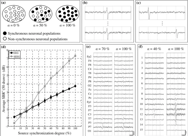
4.2 Scenario 2: synchronization degree of the source

In this scenario, we considered a single patch of 7 cm², located at the temporo-parieto-occipital junction, as in scenario 1. This patch consisted in N populations of neurons. In order to simulate this patch activity, we used a mixing of n synchronous and (N-n) non-synchronous “epileptic” time-courses (Fig. 3-a). Synchronous time-courses corresponded to the exact same realization of the neuronal population model output (Fig. 3-b) while non-synchronous time-courses corresponded to different realizations (with random time-shift between transient spikes at the population level, as shown in Fig. 3-c). The n populations with synchronous activity were randomly chosen according to a uniform distribution. The synchronization degree within the patch was defined as = n/N x 100. For each varying from 0 to 100%, by step of 10%, an average

SBR* _{value was estimated from signals simulated for 50}

different random draws of the n synchronous populations inside the patch, in order to account for the population position variability.

Results are displayed in Fig. 3-d. The average of SBR*

values (over the 50 random draws) increased both for scalp and depth EEG, as the patch synchronization intensified. The slope of the curve was steeper for depth EEG than for scalp EEG and, from a 20% synchronization, average SBR* _{values measured for}

depth EEG signals were found to be higher than those measured on scalp EEG signals. As an example, an average SBR* _{value of 3 dB was reached for = 40% in}

depth EEG signals while this same value was reached for = 78% in scalp EEG signals. It is noteworthy that for a given synchronization degree, the standard deviation of the average SBR* _{value was higher for}

Fig. 2: Scenario 1 – influence of the source spatial extent. (a) The epileptic patch was located in left temporo-parieto-occipital region, with a spatial extent S varying from 1 cm² to 50 cm². (b) The same time-course (interictal spike) was assigned to all dipoles within the epileptic patch. (c) Evolution of the average SBR (SBR*_{) with respect to the source spatial extent, for scalp (black line) and depth (grey line) EEG signals. (d) Simulated scalp EEG}

signals for three spatial extents (7, 18 and 32 cm²). Only 19 from the 63 channels are presented here (10-20 standard system). (e) Simulated depth EEG signals for three spatial extents (3, 9 and 24 cm²).

Figs. 3-e and 3-f present examples of simulated scalp and depth EEG signals, respectively. Epileptic spikes became clearly visible for = 70% (respectively 40%) on scalp EEG signals (respectively depth EEG signals), and their amplitude gradually increased with the patch synchronization degree, in both cases.

5. Discussion

In this study, an attempt was made to quantitatively investigate the relationship between EEG signals (both scalp and depth) and the spatio-temporal configuration of the underlying neuronal sources. This issue was addressed through a realistic model of EEG generation. The proposed model relies on a spatio-temporal representation of the neuronal sources of activity, which combines a distributed dipole source model (anatomically realistic description of the spatial features of the sources) and a model of coupled neuronal populations (physiologically relevant simulation of the time-courses associated to the dipole sources).

The model was used, in the particular context of epileptiform activity (interictal spikes), to establish relations between source-related parameters (spatial extent, synchronization) and the simulated scalp and depth EEG signals (amplitude of the spikes, amplitude gradient along intracerebral electrodes, topography over scalp electrodes).

As far as the influence of the spatial extent of the source is concerned, our results show that the area of cortex involved in the generation of interictal spikes is rather large. Although this result has already been suggested by several studies [7,8,9], we were able to accurately quantify the contribution of a “focal” epileptic source of a given area to the amplitude of resulting spikes observed in EEG signals. Results also illustrate a high sensitivity of depth EEG, which can detect the activity arising from smaller cortical areas as compared to scalp EEG. In addition to the source spatial extent, the influence of the source geometry is also well illustrated in scenario 1, particularly in depth EEG signals. As the area of the epileptic patch was progressively increased, the maximum amplitude of the spike initially observed

…

Source spatial extent (cm²)

A ve ra ge S B R (S B R *) (d B ) (b) Fp2 F4 F8 C4 T8 P4 P8 O2 Fz Cz Pz Fp1 F3 F7 C3 T7 P3 P7 O1 1 2 3 4 5 6 7 8 9 10 11 12 13 14 15 S = 7 cm² S = 18 cm² S = 32 cm² (d) 1 2 3 4 5 6 7 8 9 10 11 12 13 14 15 S = 3 cm² S = 9 cm² S = 24 cm² (e) 1 s 10 0 V 1 s 1 m V

Fig. 3: Scenario 2 – influence of the source synchronization degree. (a) The synchronization degree is defined as the proportion, inside the patch, of neuronal populations with synchronous epileptic activity (black dots, (b)) vs. non-synchronous epileptic activity (white dots, (c)). (d) Evolution of the average SBR* (SBR* averaged over 50 random draws) with respect to the patch synchronization degree, for scalp (black line) and depth (grey line) EEG signals. For each point, the bar indicates the standard deviation obtained for 50 random draws. (e) Simulated scalp EEG signals for two synchronization degrees (70 and 100%). (f) Simulated depth EEG signals for two synchronization degrees (40 and 100%).

on the lateral contact of the electrode moved towards a more mesial contact even if the barycentre of the patch remained the same. In that case, the increase of the spatial extent of the cortical patch most likely implies a modification of its geometry and thus, of its global contribution to the recording contacts. As far as the scalp EEG signals are concerned, results obtained in scenario 1 show a lower sensitivity to the source geometry (as expected). Indeed, since scalp electrodes are relatively far from brain sources, their volume of sensitivity is greater when compared to intracerebral sensors.

We also addressed the issue of the degree of synchronization between neuronal populations within the epileptic source. Results show clear differences in the influence of this parameter on simulated scalp and depth EEG signals. On the one hand, scalp-recordable epileptic spikes (with a SBR* _{higher than 3 dB) were}

obtained for relatively high values of the degree of synchronization (superior to 70%). This result corroborates those already reported and suggesting that only widely synchronized cortical activities are observed on the scalp [10]. On the other hand, results show that epileptic spikes corresponding to low synchronization degree (around 40%) could be observed in simulated depth EEG signals. Modeling results thus indicate that depth EEG signals can reflect epileptic activities corresponding to a weak and partial synchronization between neuronal populations forming the epileptic patch.

6. Conclusion

The model we have developed not only allows for the simultaneous simulation of signals collected on scalp and depth electrodes, but also allows for the analysis of simulated signals with respect to the configuration of underlying sources of activity. However, although our model provided insights into the relationship between EEG data and the configuration of neuronal sources, it still suffers from some limitations. Like most physiological models, it can only approximate natural phenomena because the underlying biophysical and bio-mathematical description is imperfect. In particular, for depth EEG, when the electrode contact is very close to the source, the applicability of the dipole theory can be questioned. In addition, the neuronal population model we used to represent the time-varying intensity of dipoles was reduced to its simpler form (one sub-population of pyramidal cells and one sub-sub-population of local interneurons). In actual neocortex, the cellular organization is obviously more complex. Another drawback is that the model does not account for the contribution of subcortical structures to signals recorded by electrodes. This question, which is still highly debated among the neuroimaging community, is crucial in certain types of epilepsy like temporal lobe epilepsy. We think that progress can still be made in “decoding” the information conveyed by EEG signals, particularly by better understanding the relationship between the properties of signals recorded by electrodes (both scalp and depth) and the spatio-temporal organization of the

= 0 %

(a)

Synchronous neuronal populations Non-synchronous neuronal populations

Source synchronization degree (%)

A ve ra ge S B R * (5 0 dr aw s) ( dB ) Fp2 F4 F8 C4 T8 P4 P8 O2 Fz Cz Pz Fp1 F3 F7 C3 T7 P3 P7 O1 = 70 % = 100 % (d) 1 2 3 4 5 6 7 8 9 10 11 12 13 14 15 = 50 % = 100 %

…

neuronal sources that produce these signals. This work is a first step into this direction. The present study was carried out in the particular context of epilepsy. However, this approach could be adapted to other fields of EEG-based research, in which the relationship between the properties of recorded EEG signals and the spatial extent, geometry, synchronization level and temporal dynamics of the underlying generators is often questioned.

Acknowledgements

This work was supported in part by the French Ministry of Research (ACI Neurosciences Intégratives et Computationnelles 2002-2006).

References

[1] Cosandier-Rimélé D, Badier JM, Chauvel P, Wendling F. A physiologically plausible spatio-temporal model for EEG signals recorded with intracerebral electrodes in human partial epilepsy. IEEE

Trans Biomed Eng, 54(3), 2007, 380-388.

[2] Cosandier-Rimélé D, Merlet I, Badier JM, Chauvel P, Wendling F. The neuronal sources of EEG: Modeling of simultaneous scalp and intracerebral recordings in epilepsy. Neuroimage, 42, 2008, 135-146. [3] Dale AM, Sereno MI. Improved localization of cortical activity by combining EEG and MEG with MRI cortical surface reconstruction: a linear approach. J Cogn Neurosci, 5, 1993, 162-176.

[4] Wendling F, Bellanger JJ, Bartolomei F, Chauvel P. Relevance of nonlinear lumped-parameter models in the analysis of depth-EEG epileptic signals. Biol Cybern, 83(4), 2000, 367-378.

[5] Gonçalves SI, de Munck JC, Verbunt JP, Bijma F, Heethaar RM, Lopes da Silva F. In vivo measurement of the brain and skull resistivities using an EIT-based method and realistic models for the head. IEEE Trans Biomed Eng, 50(6), 2003, 754-767.

[6] Hämäläinen MS, Sarvas J. Realistic conductivity geometry model of the human head for interpretation of neuromagnetic data. IEEE

Trans Biomed Eng, 36(2), 1989, 165-171.

[7] Ebersole JS. Defining epileptogenic foci: past, present, future. J

Clin Neurophysiol, 14(6), 1997, 470-483.

[8] Merlet I, Gotman J. Reliability of dipole models of epileptic spikes. Clin Neurophysiol, 110(6), 1999, 1013-1028.

[9] Alarcón G, Kissani N, Dad M, Elwes RD, Ekanayake J, Hennessy MJ, Koutroumanidis M, Binnie CD, Polkey CE. Lateralizing and localizing values of ictal onset recorded on the scalp: evidence from simultaneous recordings with intracranial foramen ovale electrodes.

Epilepsia, 42(11), 2001, 1426-1437.

[10] Cooper R, Winter AL, Crow HJ, Walter WG. Comparison of subcortical, cortical and scalp activity using chronically indwelling electrodes in man. Electroencephalogr Clin Neurophysiol, 18, 1965, 217-228.