Corrosion modelling of iron for long term prediction in nuclear waste repository

HAL Id: cea-02442344

https://hal-cea.archives-ouvertes.fr/cea-02442344

Submitted on 16 Jan 2020

HAL is a multi-disciplinary open access archive for the deposit and dissemination of

sci-L’archive ouverte pluridisciplinaire HAL, est destinée au dépôt et à la diffusion de documents

Corrosion modelling of iron for long term prediction in

nuclear waste repository

Julia Agullo, Christian Bataillon, Laurent Trenty

To cite this version:

Julia Agullo, Christian Bataillon, Laurent Trenty. Corrosion modelling of iron for long term prediction in nuclear waste repository. EUROCORR 2016 - European Corrosion Congress, Sep 2016, Montpellier, France. �cea-02442344�

Corrosion modelling of iron for long term prediction in

nuclear waste repository

Julia AGULLO1, Christian BATAILLON2, Laurent TRENTY3

1_{Den-Service de la Corrosion et du Comportement des Matériaux dans leur Environnement}

(SCCME), CEA, Université Paris-Saclay, F-91191, Gif-sur-Yvette, France, julia.agullo@cea.fr

2_{Den-Service de la Corrosion et du Comportement des Matériaux dans leur Environnement}

(SCCME), CEA, Université Paris-Saclay, F-91191, Gif-sur-Yvette, France, christian.bataillon@cea.fr

3_{Andra, DRD, EAP, 1-7 rue Jean Monnet 92290 Chatenay-Malabry, France,}

laurent.trenty@andra.fr

Abstract: The long-term behavior of nuclear waste canisters in geological repository depends on metallic materials and geochemical features of the surrounding. In clay, H₂ and metallic cations induce geochemical transformations which change pH and redox potential. So the 1000-years behavior of canisters could be predicted by linking geochemical and corrosion models.

The Diffusion Poisson Coupled Model (DPCM) has been proposed as corrosion model for passive iron. To ensure feedback from geochemistry on corrosion rate, backward reactions were introduced. The DPCM is a mechanistic model involving 40 parameters to solve the Poisson and Fick equations in moving boundaries situation. The purpose of this paper is to present the strategy adopted to set up parameters of the CALIPSO code which solves the equation of the DPCM.

It has been shown that one half of these parameters could be evaluated from equilibrium considerations. Then specific experiments could be simulated to set up some parameters. For instance, dissolution rate of magnetite layer monitored by XANES, layer thickness growth monitored by ellipsometry, potentiostatic and Mott-Schottky experiments have been simulated to set up parameters of: dissolution and release processes, inner oxide growth and electrostatic description of outer interface. This strategy was efficient because the DPCM can simulate a large panel of stationary and non-stationary experiments.

Introduction

The long-term behavior of nuclear waste canisters in geological repository depends on metallic materials and geochemical features of the surrounding. In clay, H₂ and metallic cations induce geochemical transformations which change pH and redox potential. So the 1000-years behavior of canisters could be predicted by linking geochemical and corrosion models.

The Diffusion Poisson Coupled Model (DPCM) has been proposed as corrosion model for passive iron. To ensure feedback from geochemistry on corrosion rate, backward reactions were introduced as shown on figure 1. The DPCM is a mechanistic model involving 40 parameters to solve the Poisson and Fick coupled equations in moving boundaries situation.

This model is explained in detail in reference [1]. In summary, the DPCM model describes an oxide layer which contains mobile charges (electrons and ionic species). The boundary conditions of the oxide layer are described by kinetic equations in order to solve the Fick equations and by equations describing the state of electric charge of adjacent phases of the oxide layer to the resolution of the Poisson equation. Two particular kinetic steps monitor independently the movement of interfaces of the oxide layer (metal ≡ inner and oxide-environment ≡ outer). Thereby, the locations of interfaces are unknown in the DPCM model. The CALIPSO code solves the equations of the Diffusion Poisson Coupled Model. The numerical methods implemented in the CALIPSO code are described in detail in reference [2]. In summary, these methods are based on a fully implicit resolution of coupling between Fick, Poisson and moving interfaces equations. This implementation solves the DPCM model in either steady state or dynamic situation. A finite volume scheme with a discretization of

The purpose of this paper is to present the strategy adopted to set up parameters of the CALIPSO code associated to the DPCM. Some parameters like diffusion coefficients [3] are available in literature. For estimation of others parameters, several ways were considered: thermodynamic equilibrium and some specific experiments dedicated to elementary fluxes like reductive dissolution of magnetite, steady state passive current measurements or oxide layer growth ellipsometry monitoring.

Thermodynamic equilibrium

Description of the system

Considering the equilibrium reaction (1):

Fe3+

+ 3

2 H2 →← Fe + 3 H

+

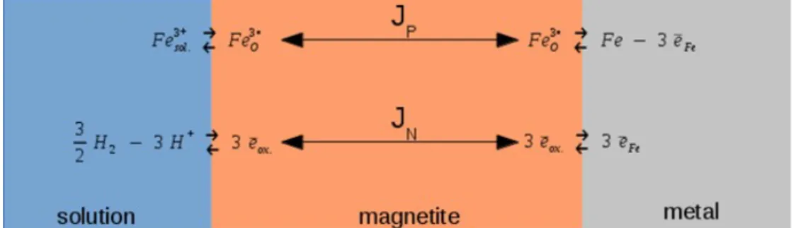
(1) The difference of potential, E, between the metal and the solution corresponds to an equilibrium electrochemical potential. This equilibrium could be divided in 2 parallel reaction paths as depicted in figure 2: one for the cations and another for the electrons. In the framework of kinetic any equilibrium can be considered as a steady state where backward and forward paths run as the same rate.

Each path could be considered as an electrochemical equilibrium which are referenced in the literature as standard potential. In the anodic part:

Fe →_{← Fe}3+ + 3 e (2) In the cathodic part:

3

(

H+ + e →_← 1

2H2

)

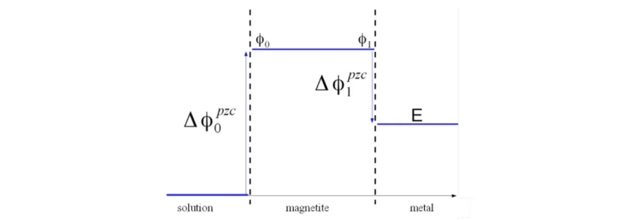
(3)

It must be outlined that for electrochemical equilibrium the potential in all phases are homogeneous. Moreover interfaces are always assumed to be uncharged. Hence the voltage drop between the adjacent phases are the so-called potential of zero charge (PZC). Finally the global potential between the solution and metal is the electrochemical potential from the Pourbaix diagram [4]. The potential profile in the system solution/magnetite/metal of figure 2 at the chemical equilibrium (1) is presented in figure 3.

Electronic equilibrium of solution/magnetite/iron system

In the DPCM model, the kinetic of the electronic exchange between the iron and the oxide is described by the following equation:

Je = me1c1e − ke1cemetal (4)

where ce1 and cemetal are the electron concentrations in the oxide at the inner interface and

in metal, respectively. me1 and k1e are the kinetic constants of Richardson.

me1 =

√

k_BT 2 π m* and ke 1 =

√

kBT 2 π m** (5)

where m* _{et m}** _{are effective masses of electron in the oxide and in metal respectively}

and kB Boltzmann constant.

The equilibrium corresponding at Je = 0. The solution of this equation gives the

concentration of electrons in equilibrium in the oxide at the inner interface. After dimensionless this concentration by N1eq = ce1(eq) Ωox where Ωox is molar volume of the

oxide and from the integration developed in [1], the following relation is obtained:

N1eq = Nmetal ln

[

1+exp

[

−γ

(

E −φ1

)

]

]

(6)

where N_metal = Ω_oxk_BT n_DOSFe

√

m**

m* . In this expression, nDOS

Fe _{is the average density of}

state for iron. Knowing

(

E − φ₁

)

= Δ φ₁pzc (cf. figure 3), the equation (6), it is possible to calculate Δ φ₁pzc :

Δ φ₁pzc = −1_{γ ln}

[

exp

(

N1 eq

N_metal

)

−1

]

(7)

Figure 3: Potential profile in the solution/magnetite/metal system of figure 2 at the chemical equilibrium (1)

As

(

E − φ₁

)

= Δ φ₁pzc and Δ φ0pzc = φ0 = φ1 (cf. figure 3), the following relation is

obtained:

[

E (pH ) − Δ φ₀pzc

]

= Δ φ₁pzc (8)

The system described on figure 2 also corresponds to an electrochemical equilibrium between iron and magnetite:

3 Fe + 4 H2O →_{← Fe}3O4 + 8 H

+

+ 8 ̄e (9)

The potential of this equilibrium is:

E = EFe/ Fe3O4

0

− ln 10_γ pH (10) At 25°C, E0Fe/ Fe₃O₄ = -0.085 V/NHE (Normal Hydrogen Electrode). In equation (8), the

potential E is the electrochemical equilibrium between iron and magnetite in contact of solution (cf. Relation (10)) and depends of pH solution. But Δ φ1

pzc

is a characteristic of iron-magnetite junction which is independent of solution pH. So Δ φ0pzc should be a pH function

and its pH dependence should be the same as potential E(pH).

In the CALIPSO code, the value of Δ φ₀pzc is calculated by the following relation:

Δ φ₀pzc(pH ) = Δ φpzc pH =0

−ln 10_{γ . npH}pzc0. pH (11)

The pH dependence of solution is monitored by the value of npH pzc0

. This dependence should be identical to the one of the Fe/ Fe3O4/H

+

couple equilibrium electrochemical potential (cf. relation (10)). Consequently, npH

pzc0

= 1. Introducing (11) and (10) in (8), the following reaction is obtained:

Δ φ_pzcpH =0 = E_{Fe/ Fe}

3O4

0

− Δ φ₁pzc with npHpzc0 = 1 (12)

It should be noted that the description of the local electronic balance at the inner interface and the fact that the potential profile in the magnetite layer is homogeneous at thermodynamic equilibrium leads to the identification of potential Δ φ1

pzc

for inner interface and Δ φ0 pzc

for outer interface. Moreover, the potential Δ φ0pzc depends on pH solution and is expressed as

an electrochemical potential with reference to the NHE potential. Until now, no data on the kinetic constants ratio values have yet been obtained because Butler-Volmer type reactions have not yet been introduced. The electronic exchange reaction between magnetite and iron does not follow a type of Butler-Volmer law but a law of Richardson. In the following paragraphs, Butler-Volmer type law will be introduced.

The kinetics of the electronic exchange between the oxide and the solution is the kinetic redox of H+_/H 2 couple: J_e = m_e0_a H2 ne H2 exp

₍

b_e0 γ φ₀

)

− k_e0₁₀−ne pH . pH _c e 0 _exp

(

−a_e0 γ φ₀

)

(13)

At the equilibrium, Je = J0 . After rearranging the following relation is obtained: ke 0 m_e0 = Ωox 10 [n_epH_−(a e 0_+b e 0_{)]. pH} exp

[

−

(

a_e 0 +b_e0

₎

γ Δ φ₁pzc

]

N₁eq(Δ φ₁pzc) . exp

[

[

(

ae 0 +b_e0

)

−2 n_eH2

]

_γE Fe/ Fe3O4 0

]

(14)

In this relation, the left part is a kinetic constants ratio and is pH independent. So it implies that:

n_epH

=

(

a_e0

+b0_e

)

(15)

The following relation, which is a constant, is finally, obtained:

ke 0 m_e0 = Ωox exp

[

−n_epH γ Δ φ₁pzc

]

Nmetalln

[

1 + exp

(

Δ φ1 pzc

)

]

exp

[

[

ne pH −2 ne H₂

]

γEFe/ Fe3O4 0

]

(16)

The relation (16) does not define a unique solution since it depends on the choice of the reactions of orders ne

pH

and n_eH2 . In the case of a local electrochemical balance it is useful

to take as orders reactions the values of the stoichiometric coefficients of the reaction (3). A convenient solution would be:

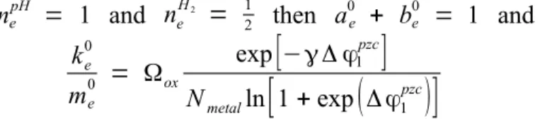
nepH = 1 and ne H2 ₌ 1 2 then a0e + be0 = 1 and k_e0 me 0 = Ωox exp

[

−γ Δ φ1pzc

]

N_metalln

[

1 + exp

(

Δ φ₁pzc

)

]

(17)

The ratio of kinetic constants depends only on the potential of zero charge of the inner interface and the concentration dimension. The sum of the Butler -Volmer coefficients is equal to 1. This is an expected result for the redox process of the H+_/H

2 couple since reactant and

product are species in solution.

The same processing could be applied for the Fe3+_{/Fe couple. And finally the description of}

the thermodynamic equilibrium with the DPCM leads to the following relation listed in the Table 1.

Table 1: Kinetic constants ratio for interfacial reactions for solution/magnetite/iron system described in figure 2.

Mobile charge Outer interface Inner interface

Cations mFe 0 k0Fe = 2 Pm−2 exp

[

3γ

₍

E_Fe/Fe3+ 0 _{− Δ φ} 1 pzc

)

]

a1 0 +b1 0 = 1 mFe 1 kFe 1 =

(

Pm 2 −1

)

exp

[

3

(

a1 L_+b 1 L

)

γ Δ φ₁pzc

]

Electrons ke 0 me0 = Ω_oxexp

[

γ

(

E_H+ /H2 0 _{− Δ φ} 1 pzc

)

]

nepH = ae0+be0 = 1 ke 1 me1 =

√

m ** m*

XANES study of the cathodic reduction of artificial iron oxide passive films [5]

Schmuki et al. have studied the galvanostatic reduction of Fe2O3 and Fe3O4 sputter deposited

thin films by XANES (X-ray Absorption Near Edge Spectroscopy) [5]. Two informations are available in Fig 8 herein [5] that is the thickness and the potential evolution with the charge density. As the current density was constant (-5µA/cm2_{), the charge density could be}

converted in time. In the framework of the DPCM, this experimental set up could be described by the figure 4.

In this figure, the ferric release reduction can be discarded since the potential is very cathodic. As the film has been deposited by sputtering, oxygen vacancies are likely very low and as there is no growth between magnetite and tantalum, therefore the oxygen vacancies flux can be discarded. As consequences the experience is monitoring by 2 independent steps. The Oxide Host Lattice Dissolution which is linked with the thickness decrease and the constant

ke0 which is linked to the potential drop during the reduction. It must be highlighted that the

kinetic constant for electronic exchange must be those of the junction between magnetite and tantalum. The nDOSTa should take into account in the paragraph on the Electronic equilibrium

of solution, magnetite iron system. Both interfacial reactions depend on the pH being that of the pH buffer (8.4).

Oxide Host Lattice Growth reaction

The rate of the oxide growth at the inner interface (cf. figure 1) determines the motion rate of this interface. The motion rate of the outer interface was determined previously. When both motion rate are equal steady state is achieved. In the literature [6], the variation of the steady state thickness as the applied potential is available (figure 9 herein [6]). It has been assumed that the process is irreversible as in the Point Defect Model [6]. As the oxide growth rate depends on the inner interfacial potential this is obvious that this rate depends on the applied

potential through the resolution of the Poisson equation which defines the potential profile in the system. This could be simulated by the CALIPSO code in searching for values of kox

1

(cf. figure 1) and the associated Butler-Volmer coefficient ( aox1 ) in order to fit the

experimental curves available in [6]. This is important to notice that this set up is likely the more difficult to achieve since in practice the thickness range could be easily got but the right slope not due to the potential dependence.

Conclusions

In this paper a strategy of the CALIPSO set up organised step by step allowing to estimate parameters values without using multifitting processing which is often tricky to implement as soon as the number parameters increased over 3 or 4. The first step was based on equilibrium states which allowed to reduce the number of independent parameters since kinetic constant ratio are constant. In the second step, the dissolution rate of the oxide at the outer interface is available from the literature. It is the major parameter linked to the pH of depassivation or Flade potential. Knowing the potential and pH ranges were passive film exist in the third step, the variation of the steady state thickness with applied potential has allowed to estimate the parameter value of the oxide growth. From this point, the last step is to set up the value for k0Fe (figure 1) which controls the level of the anodic passive current. Until now the

parameters set up was based on data and experiments which did not deal with corrosion situation. Then it is possible to check of the parameters values set in simulating a corrosion experiment using the evolution of the free corrosion potential and the final damage.

Acknowledgement

The authors would like to thank Andra for financial support.

References

1. C. Bataillon, F. Bouchon, C. Chainais-Hillairet, C. Desgranges, E. Hoarau, F. Martin, S. Perrin, M. Tupin, J. Talandier, Corrosion modelling of iron based alloy in nuclear waste repository, Electrochimica Acta 55 (2010) 4451-4467.

2. C. Bataillon, F. Bouchon, C. Chainais-Hillairet, J. Fuhrmann, E. Hoarau, R. Touzani, Numerical methods for the simulation of a corrosion model with moving oxide layer, Journal of Computational Physics 231 (2012) 6213-6231.

3. M. Backhaus-Ricoult, R. Dieckmann, Defects and Cation Diffusion in Magnetite (VII): Diffusion Controlled Formation of Magnetite During Reactions in the Iron-Oxygen System, Berichte der Bunsengesellschaft für physikalische Chemie 90 (1986) 690-698.

4. M. Pourbaix, Atlas of Electrochemical Equilibria in Aqueous Solutions, National Association of Corrosion Engineers 1974.

5. P. Schmuki, S. Virtanen, A.J. Davenport, C.M. Vitus, In Situ X‐Ray Absorption Near‐Edge Spectroscopic Study of the Cathodic Reduction of Artificial Iron Oxide Passive Films, Journal of the Electrochemical Society 143 (1996) 574-582.

6. Z. Lu, D.D. Macdonald, Transient growth and thinning of the barrier oxide layer on iron measured by real-time spectroscopic ellipsometry, Electrochimica Acta 53 (2008) 7696-7702.