HAL Id: hal-02180617
https://hal.inria.fr/hal-02180617
Submitted on 11 Jul 2019
HAL is a multi-disciplinary open access
archive for the deposit and dissemination of
sci-entific research documents, whether they are
pub-lished or not. The documents may come from
teaching and research institutions in France or
abroad, or from public or private research centers.
L’archive ouverte pluridisciplinaire HAL, est
destinée au dépôt et à la diffusion de documents
scientifiques de niveau recherche, publiés ou non,
émanant des établissements d’enseignement et de
recherche français ou étrangers, des laboratoires
publics ou privés.
Acoustic Evaluation of Simplifying Hypotheses Used in
Articulatory Synthesis
Ioannis Douros, Yves Laprie, Pierre-André Vuissoz, Benjamin Elie
To cite this version:
Ioannis Douros, Yves Laprie, Pierre-André Vuissoz, Benjamin Elie. Acoustic Evaluation of Simplifying
Hypotheses Used in Articulatory Synthesis. ICA 2019 - 23rd International Congress on Acoustics, Sep
2019, Aachen, Germany. �hal-02180617�
Acoustic Evaluation of Simplifying Hypotheses Used in Articulatory Synthesis
Ioannis Douros(1), Yves Laprie(1), Pierre-André Vuissoz(2), Benjamin Elie(3)
(1)Loria/CNRS/Inria, France, yves.laprie@loria.fr
(2)Université de Lorraine, INSERM U1254, IADI, France, pa.vuissoz@chru-nancy.fr (3)IMSIA, Ensta, France, benjamin.elie@ensta.fr
Abstract
Articulatory synthesis allows the link between the temporal evolution of the Vocal Tract (VT) shape and the acoustic cues of speech sounds to be investigated unlike other approaches of speech synthesis. A number of simplifying assumptions have to be made to enable the speech signal to be generated in a reasonable time. They mainly consist of approximating the propagation of the sound in the vocal tract as a plane wave, approximat-ing the 3D VT shape from the mid-sagittal shape, and simplifyapproximat-ing the vocal tract topology by removapproximat-ing small cavities. This work is dedicated to the evaluation of these assumptions. For this purpose 3D MRI VT shapes for sustained vowels and fricatives were acquired together with the speech sound recorded via an optical mi-crophone. Vocal tract resonances were evaluated from the 3D acoustic simulation computed with the K-wave Matlab package from the complete 3D VT shape and compared to those of real speech, those provided by sim-plified 3D VT shapes (near epiglottis), and those provided by either the electric simulation from the mid-sagittal shape, or the 2D K-wave package from a mid-sagittal VT shape. We will exploit these results to improve the simplified acoustic simulations used in articulatory synthesis.
Keywords: Speech, Acoustics, Simulations, 3D MRI
1
INTRODUCTION
Speech synthesis has reached a high level of naturalness through concatenative approachesand more recently deep learning approaches. Both are based on the use of a large corpus of pre-recorded speech.
The speech corpus has to cover all phenomena that are to be treated. Hence, the more phonetic contexts, speech styles, expressions, speaker postures, etc the corpus covers, the more natural the synthesized speech. All this contributes to increasing the size of the corpus.
On the other hand the weakness of those techniques is tightly connected to their dependence on the corpus. This means that changing the speaker characteristics, adding new expressions, or taking into account speech production disorders is almost impossible. These techniques do not contribute to the understanding of speech production and are unable to link an acoustic cue, for example the evolution of frequencies in the vicinity of a consonant, to their articulatory origin.
Unlike these approaches, which only model the result of speech production, i.e. the acoustic speech signal, articulatory synthesis [1]–[3] explicitly models the link between the vocal tract, vocal folds and aero-acoustic phenomena. This is achieved by solving the equations of aerodynamics and acoustics in the vocal tract and by using its geometry as an input. It should be noted that to facilitate resolution, a plane wave is assumed to propagate from the glottis to the lips. This simplification is widely used from a practical point of view, although its precise scope is partly unknown.
The geometry of the vocal tract results from the position of the speech articulators, and thus from the activity of corresponding muscles. A first solution to model these phenomena is to use biomechanical modeling to compute the shape of all the deformable speech articulators [4], [5]. This involves modeling the behaviour of muscles and the properties of muscle tissues in a realistic way before solving the mechanical equations. Despite
constant progress, this approach is often limited to predicting the position of the jaw and the tongue shape and it is still unimaginable to use a biomechanical approach to calculate the whole shape of the vocal tract. For these reasons we prefer to use an articulatory model [6], [7] to compute the vocal tract geometry. Of course, the articulatory model must provide a geometric description close to reality in order to guarantee a good quality of synthesis. Similarly to the biomechanical approach, one of the challenges consists of collecting and processing data to construct the model. As the delineation of the articulators in the MRI images is a task that requires a certain amount of interpretation of the geometry of the vocal tract and has a very long processing time, it is often preferable to construct a two-dimensional model in the mid-sagittal plane and then calculate the transverse area at each point of the vocal tract from the glottis to the lips [8].
To know the impact of the articulatory model and its use in articulatory synthesis, we therefore studied three questions. The first is the choice of a 2D or 3D model by comparing the synthesis obtained from a 3D volume, from a 2D sagittal slice completed by the approximation of the 3rd dimension, or finally from a 2D plane wave with an electric analogy. The second question is whether it is possible to simplify the mid-sagittal slice at the level of epiglottis and uvula. These approximations are often made because they avoid including additional cavities in the calculations. The last question is related to the speaker’s position in the MRI machine. This question is important because the model and acoustic calculations are related to the position the subject adopted during the recording. This position can change between two sessions and it can also change because another MRI machine may have been used.
2
MATERIALS AND METHODS
2.1 Data acquisition
For the purpose of this study, we used MRI data part of a study approved by an ethics committee and the subject gave written informed consent (ClinicalTrials.gov identifier: NCT02887053). The subject used for the data acquisition is a healthy male French native speaker at the age of 32, without any reported speaking or hearing problems.
The MRI data was acquired on a Siemens Prisma 3T scanner (Siemens, Erlangen, Germany) with gradient of 80mT /m amplitude and 200mT /m/ms slew rate. We used the 3-dimensional cartesian vibe sequence (T R = 3.75 ms, T E = 1.43, FOV = 199 × 220 mm, f lip angle = 9 degrees) for the acquisition. The pixel bandwidth is 445Hz/pixel with an image resolution of 256 × 174. Scan slice thickness is 1.2 mm and the number of slices is 120. The pixel spacing is 0.8597 and the acceleration factor is 3 iPAT . The acquisition time was 7.4 s which allows the subject to maintain phonation easily.
The subject’s vocal tract was imaged while he lay supine in the MRI scanner. The recording time for the subject, including calibration and pauses between phonemes, was 2 hours.
Audio was recorded at a sampling frequency of 16 kHz inside the MRI scanner using FOMRI III (Optoacous-tics, Or Yehuda, Israel) fiber optic microphone. The subject starts producing the phoneme just before the MRI recording starts and sustains phonation until the end of the acquisition. The subject wears ear plugs for pro-tection from the scanner noise, but is still able to communicate orally with the experimenters via an in-scanner intercom system.
Since the sound is recorded at the same session of the MRI acquisition, there is additional noise in the audio signal. In order to de-noise it, we used the de-noising algorithm proposed in [9]. The main idea of the algorithm is based on three steps.
1. Computation of the covariance matrix of the noisy signal.
2. Applying Maximum Likelihood in order to estimate the model parameters from the covariance matrix and a set of pre-computed models.
We apply this algorithm to our data using the FASST toolbox [10]. 2.2 Segmentation
For the purposes of our experiments, we used the ITK-SNAP software [11] to segment the volume of the vocal tract. ITK-SNAP provides a great variety of tools for segmenting images, both automatically and manually. As far as automatic segmentation is concerned, ITK-SNAP implements two active contour segmentation algo-rithms, region competition and geodesic active contours.
ITK-SNAP also provides the option to use some image processing filters like thresholding the image. At the next step, the user should specify the initial surface or "seeds" that will eventually expand to cover the whole segmentation structure. The user can set multiple "seeds" corresponding to the same structure, and as the seeds evolve during the segmentation process, they will eventually unify and form one region. The fourth and last step is to specify the parameters of the equation which control how the "seeds" are stretching. Different selections of parameters will result in changes at the evolution speed or at the behaviour of the contour when it approaches the boundaries. The automatic segmentation algorithms can be applied both to 2D and 3D images.
For manual segmentation, ITK-SNAP offers two types of tools. The first one is some polygon-based tools where the user draws dots and the dots are connected with a line to form the segmentation region. The second one is using a variety of shapes of brushes to paint the segmentation region. The most interesting among them is the adaptive brush that adjusts itself to follow the image boundaries. The brush tool can be used for both to 2D and 3D image segmentation.
2.3 Acoustic simulation
For the acoustic simulations, we employ the k-wave Matlab toolbox [12]. This toolbox has a wide range of applications like photoacoustic tomography, ultrasound wave propagation, and acoustic propagation [13]. Several numerical methods have been developed to solve the partial differential equations of acoustics, like finite differences, finite elements, and boundary element methods [14]. These methods offer significant advantages as they can calculate acoustic characteristics accurately and implement frequency dependent losses at boundaries. However, in many cases these methods are significantly slow. This happens due to the fact that they require a small time step to achieve a good accuracy and a lot of grid points per wave length. In the method used by k-wave these problems are solved by interpolating a Fourier series through all of the grid points in order to get the estimation of the gradient. This approach solves the problems of the previously referred methods as it a) requires fewer grid points (only two) per wave length since the base function of the Fourier series is the sinusoid and b) it can be fast since it employs Fast Fourier Transform (FFT) to calculate the amplitudes of the simulated signals. A problem that arises is that when a wave approaches the computational grid boundaries, it keeps propagating to the medium by entering from the opposite site of the computational grid. This happens because of the usage of the FFT algorithm for the computation. To tackle this issue, k-wave adds a specific type of layer to the boundaries of the computational grid by implementing an absorbing boundary condition, called Perfect Match Layer (PML), which prevents this phenomenon.
Finally, k-wave toolbox has a great number of parameters that can be customised for a simulation, most of them concerning the grid and time sparsity, the properties of the mediums, the sensors, the sources, the number of dimensions (1D/2D/3D), the number of PML, etc.
2.4 Electrical simulation
To perform the electrical simulation we used some of the tools provided from the Xarticul software [15]. Xar-ticul offers multiple tools like an easy way to delineate and process arXar-ticulator contours, semi-automatic artic-ulatory measurements and construction of articartic-ulatory models [16]. Xarticul can perform acoustic simulations from the area function by using the algorithm proposed in [17] which is based on the Transmission Line Circuit Analog (TLCA) method [18].
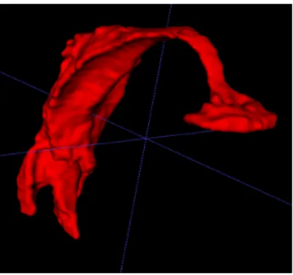
Figure 1. 3D volume of /i/ vowel
3
EXPERIMENTS
We present the way we prepared data for acoustic simulations for the three addressed issues and present results for the comparison between 2D and 3D only due to space constraints.
3.1 Image segmentation for investigating the impact of 2D or 3D simulations
For the purposes of our experiments, we used five of the vowels from the database described in the previous section, /a, œ, i, o, u/. First, we processed the images with 3DSlicer [19] (http://www.slicer.org) to apply lanc-zos interpolation in order to make corrections to the image’s axis. Then, we used the tools provided by the ITK-SNAP software to automatically segment the 3D volume of the vocal tract and afterwards, we manually corrected the result. The area of interest begins at the glottis and extends to the lips, at the point where the lips stop being simultaneously visible at the coronal plane. We used two classes and 10000 points as nearest neighbours in order to assign each point to the appropriate class for the creation of the probabilistic map, and 10 balls on average per vowel as "seeds" with various sizes based on the region of the vocal tract where they were placed. Then we applied the active contour algorithm which required between 300 − 500 iterations to cover the whole vocal tract. The amount of iterations is greatly based on the vowel and the initial number, size and position of the "seeds". For the manual segmentation we used the adaptive brush tool with the default parameters to acquire the vocal tract mesh (see Fig. 1). Finally we used Meshlab [20] to smooth every mesh by applying Laplacian smoothing filter with step 3. For each vowel, about 4 hours of processing was required, with the biggest amount of time spent on the manual segmentation step.
3.2 Image preparation for investigating the impact of the subject’s position in the MRI machine
The data that we used for the experiment is 3D MRI data of the vocal tract of five vowels of French language /a/, /œ/, /i/, /o/, /y/, in three different head positions: up, natural and down. Using tools provided by ITK-SNAP, we manually segmented the vocal tract of the mid-sagital slice. We then used meshlab [20] to apply Laplacian smoothing filtering with a step of 3 to all the images.
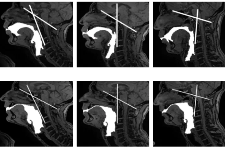
In order to measure the head position, we used the measurement proposed in [21]. The main idea is to use an angle defined by two lines to define the head position. The first line is the one that connects the interior edge of the C2-C3 cervical vertebrae. The second line is the one that connects the posterior tip of the spinous process of C1 and the tuberculum sella. As shown in Fig. 2, number 1 corresponds to the first line, number 2 corresponds to the second line, while number 3 corresponds to the calculated angle. We used imageJ software [22] to manually specify the lines and make the angle computations. The average angle was 144.8 ± 0.6°, 124.7 ± 0.8°, 101.3 ± 1.1°for the up, normal and natural position respectively. Since there is at least 20°of difference between the three positions, we were expecting to notice some difference in phonation [23].
Figure 2. 2D segmentation of /o/ (top row) and /i/ (bottom row) vowels at up, normal and down position from left to right. Lines 1 and 2 are used to define the angle 3 of the head position
3.3 Editing the mid-sagittal geometry at the epiglottis and uvula
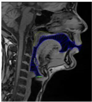
In order to investigate the impact of vocal tract shape simplifications we created three more segmentation ver-sions for every mid-sagittal slice by editing the segmented images (4 images per vowel in total with the orig-inal). In the first version we removed the epiglottis, in the second we used a constant wall approximation at velum (by removing the uvula) and in the third version we combined both simplifications (Fig. 3). These three versions of every vowel along with the original were fed into the simulations.
3.4 Acoustic simulations
For the acoustic simulations, we used k-wave toolbox for Matlab [12]. For every vowel examined, simulations were carried out in both 2D and 3D. First, the mesh was transformed into a volumetric representation using voxels. Then we specified the parameters for the 2D and 3D simulations. Since k-wave uses FFT, the number of grid points was set so as to have low prime factors, ideally a power of 2. For the 3D, we used a grid size of 128 × 128 × 128 grid points (sagittal × coronal × axial) with dx= dy= dz= 1mm. We also used a PML layer of 10 grid points at the boundaries of every side of the grid, to avoid the wave penetrating the opposite side, as explained in the previous section.
As a source we used a ball which emits a delta pulse of pressure, spreading equally in all directions. The source has radius of 5 grid points, amplitude 1 Pa and was placed at input of the vocal tract, which was specified manually for every vowel.
To record the simulated pressure we used a sensor placed at the end of the vocal tract. The medium proper-ties inside the vocal tract were cin= 350m/s, din= 1kg/m3 and the properties outside, i.e. in the tissues that delimit the vocal tract, were cout= 1000m/s, dout = 1000kg/m3, where cin, cout are the speed, and din, dout are the densities inside and outside the vocal tract respectively. The time step is set according to the two medium characteristics (here tissues and air) and the accepted value is 3 ∗ 10−8sec to guarantee a good stability. The amount of time steps computed was 1000001. The maximum allowed frequency of the grid was 175KHz. For the 2D case, we run the simulations on the y − z plane using a disc instead of a ball on the mid-sagittal plane of the vocal tract. All the other parameters remained the same between the two simulations. The amount of time required for the simulation of each vowel is about 75 hours for 3D, while for 2D is approximately 3 hours and 20 minutes. Finally, we calculated the transfer function of every vocal tract and computed their peak frequencies (see Tab. 1), to compare them with the formants computed with the electrical simulation.
Figure 3. The four versions of /i/ phoneme (original (top left), without epiglottis top right), without uvula (bottom left), without uvula and epiglottis (bottom right)
3.5 Electric simulations
For the electric simulations we used the mid-sagittal planes from the 3D MRI acquisition. We used Xarticul to manually delineate the articulator contours of each vowel Afterwards, we use 40 tubes (4) to estimate the area function of the vocal tract in order to compute its formants (Tab. 2.a). Finally, we used selective LPC to compute the formants of the original audio signal (Tab. 2.b).
Table 1. 2D / 3D formants computation from acoustic simulations in Hertz
F1 F2 F3 F4 /a/ 674 / 694 1349 / 1231 3169 / 2545 3642 / 3548 /œ/ 416 / 460 1444 / 1444 2499 / 2544 3471 / 3433 /i/ 337 / 304 2394 / 2207 3136 / 3237 3507 / 3473 /o/ 404 / 440 900 / 787 2728 / 2605 3433 / 2973 /u/ 401 / 422 741 / 850 1980 / 2007 2969 / 3064
Table 2. Comparison between electrical simulation frequencies and values extracted from the speech signal F1 F2 F3 F4 /i/ 280 1684 2927 3395 /o/ 491 905 2185 3448 /a/ 510 1200 2190 3325 /u/ 405 1182 2034 3422 /œ/ 408 1276 2168 3360 a. 2D formants computation from electrical simulations in Hertz
F1 F2 F3 F4 /i/ 380 2306 3193 3518 /o/ 430 732 2619 3052 /a/ 689 1296 2604 3413 /u/ 456 797 2016 3025 /œ/ 443 1335 2436 3405 b. Formant determination from original
Figure 4. Decomposition of the vocal tract into acoustic tubes
4
CONCLUDING REMARKS
The first remark concerns the sounds produced by the speaker in the MRI machine. As shown in Tab. ?? which gives the average values for French speakers, the measured values are a little far from the expected values. This is especially true for the first formant of close vowels /i,o,u/ which is higher in frequency. This would mean that the pharyngeal cavity is smaller due to the subject posture. The visual examination of the images shows a slightly shifted articulation in some cases, especially for /u/. The second remark is that there is a good agreement between the results of 2D/3D simulations and the formants F1 and F2 determined from the speech signal recorded. However, for F3 the 3D simulation turns out to give results closer to those of natural speech than those of the 2D simulation, probably because the 3D volume gives a geometry closer to the real one. The third remark concerns the comparison between the 2D/3D simulations on the one hand, and the electrical simulation on the other hand. It turns out that the electric simulation is not able to reproduce the formants with as good accuracy as the acoustic simulation. Since there is a good agreement between the 2D and 3D acoustic simulation, the most probable hypothesis is that either splitting of the vocal tract into small tubes or the estimation of the area function from the mid-sagittal shape is not completely satisfactory.
ACKNOWLEDGEMENTS
This work is supported by the ANR grant “ArtSpeech” (2015-2019).
REFERENCES
[1] A. Tsukanova, B. Elie, and Y. Laprie, “Articulatory speech synthesis from static context-aware articulatory targets”, in ISSP 2017, 2017.
[2] P. Birkholz, “Modeling consonant-vowel coarticulation for articulatory speech synthesis”, PLOS one, vol. 8, no. 4, 2013.
[3] Y. Laprie, M. Loosvelt, S. Maeda, E. Sock, and F. Hirsch, “Articulatory copy synthesis from cine x-ray films”, in Interspeech 2013 (14th Annual Conference of the International Speech Communication Association), Lyon, France, Aug. 2013.
[4] S. Fels, F. Vogt, K. Van Den Doel, J. Lloyd, I. Stavness, and E. Vatikiotis-Bateson, “Artisynth: A biome-chanical simulation platform for the vocal tract and upper airway”, in ISSP 2006, Citeseer, vol. 138, 2006. [5] P. Perrier, Y. Payan, M. Zandipour, and J. Perkell, “Influences of tongue biomechanics on speech move-ments during the production of velar stop consonants: A modeling study”, JASA, vol. 114, no. 3, pp. 1582– 1599, 2003.
[6] P. Badin, G. Bailly, L. Revéret, M. Baciu, C. Segebarth, and C. Savariaux, “Three-dimensional linear articulatory modeling of tongue, lips and face based on mri and video images”, Journal of Phonetics, vol. 30, no. 3, pp. 533–553, 2002.
[7] Y. Laprie and J. Busset, “A curvilinear tongue articulatory model”, in The Ninth International Seminar on Speech Production - ISSP’11, Canada, Montreal, 2011.
[8] C. Ericsdotter, “Detail in vowel area functions”, in Proc of the 16thICPhS, Saarbrücken, Germany, 2007, pp. 513–516.
[9] A. Ozerov, E. Vincent, and F. Bimbot, “A general flexible framework for the handling of prior informa-tion in audio source separainforma-tion”, IEEE Transacinforma-tions on Audio, Speech, and Language Processing, vol. 20, no. 4, pp. 1118–1133, 2012.
[10] Y. Salaün, E. Vincent, N. Bertin, N. Souviraa-Labastie, X. Jaureguiberry, D. T. Tran, and F. Bimbot, “The flexible audio source separation toolbox version 2.0”, in ICASSP, 2014.
[11] P. A. Yushkevich, J. Piven, H. C. Hazlett, R. G. Smith, S. Ho, J. C. Gee, and G. Gerig, “User-guided 3d active contour segmentation of anatomical structures: Significantly improved efficiency and reliability”, Neuroimage, vol. 31, no. 3, pp. 1116–1128, 2006.
[12] B. E. Treeby and B. T. Cox, “K-wave: Matlab toolbox for the simulation and reconstruction of photoa-coustic wave fields”, Journal of biomedical optics, vol. 15, no. 2, p. 021 314, 2010.
[13] B. E. Treeby and B. Cox, “Modeling power law absorption and dispersion for acoustic propagation using the fractional laplacian”, JASA, vol. 127, no. 5, pp. 2741–2748, 2010.
[14] H. Takemoto, P. Mokhtari, and T. Kitamura, “Acoustic analysis of the vocal tract during vowel production by finite-difference time-domain method”, JASA, vol. 128, no. 6, pp. 3724–3738, 2010.
[15] R. Sock, F. Hirsch, Y. Laprie, P. Perrier, B. Vaxelaire, G. Brock, F. Bouarourou, C. Fauth, V. Hecker, L. Ma, J. Busset, and J. Sturm, “DOCVACIM an X-ray database and tools for the study of coarticulation, inversion and evaluation of physical models”, in The Ninth International Seminar on Speech Production -ISSP’11, Canada, Montreal, 2011.
[16] Y. Laprie and J. Busset, “Construction and evaluation of an articulatory model of the vocal tract”, in EUSIPCO 2011, IEEE, 2011, pp. 466–470.
[17] B. Elie and Y. Laprie, “Extension of the single-matrix formulation of the vocal tract: Consideration of bi-lateral channels and connection of self-oscillating models of the vocal folds with a glottal chink”, Speech Communication, vol. 82, pp. 85–96, 2016.
[18] S. Maeda, “A digital simulation method of the vocal-tract system”, Speech communication, vol. 1, no. 3-4, pp. 199–229, 1982.
[19] A. Fedorov, R. Beichel, J. Kalpathy-Cramer, J. Finet, J.-C. Fillion-Robin, S. Pujol, C. Bauer, D. Jennings, F. Fennessy, M. Sonka, et al., “3d slicer as an image computing platform for the quantitative imaging network”, Magnetic resonance imaging, vol. 30, no. 9, pp. 1323–1341, 2012.
[20] P. Cignoni, M. Callieri, M. Corsini, M. Dellepiane, F. Ganovelli, and G. Ranzuglia, “Meshlab: An open-source mesh processing tool.”, in Eurographics Italian Chapter Conference, vol. 2008, 2008, pp. 129–136. [21] J. L. Perry, D. P. Kuehn, B. P. Sutton, and X. Fang, “Velopharyngeal structural and functional assessment of speech in young children using dynamic magnetic resonance imaging”, The Cleft Palate-Craniofacial Journal, vol. 54, no. 4, pp. 408–422, 2017.
[22] C. A. Schneider, W. S. Rasband, and K. W. Eliceiri, “Nih image to imagej: 25 years of image analysis”, Nature methods, vol. 9, no. 7, p. 671, 2012.
[23] M. A. Jan, I. Marshall, and N. J. Douglas, “Effect of posture on upper airway dimensions in normal human.”, American Journal of Respiratory and Critical Care Medicine, vol. 149, no. 1, pp. 145–148, 1994.