Tracking a sphere with six degrees of freedom

Publisher’s version / Version de l'éditeur:

Vous avez des questions? Nous pouvons vous aider. Pour communiquer directement avec un auteur, consultez la Questions? Contact the NRC Publications Archive team at

PublicationsArchive-ArchivesPublications@nrc-cnrc.gc.ca. If you wish to email the authors directly, please see the first page of the publication for their contact information.

https://publications-cnrc.canada.ca/fra/droits

L’accès à ce site Web et l’utilisation de son contenu sont assujettis aux conditions présentées dans le site

LISEZ CES CONDITIONS ATTENTIVEMENT AVANT D’UTILISER CE SITE WEB.

Report (National Research Council of Canada. Radio and Electrical Engineering Division : ERB), 2004-10-28

READ THESE TERMS AND CONDITIONS CAREFULLY BEFORE USING THIS WEBSITE. https://nrc-publications.canada.ca/eng/copyright

NRC Publications Archive Record / Notice des Archives des publications du CNRC : https://nrc-publications.canada.ca/eng/view/object/?id=02a62e4f-fe04-4708-a555-30f0dd3b2310 https://publications-cnrc.canada.ca/fra/voir/objet/?id=02a62e4f-fe04-4708-a555-30f0dd3b2310

NRC Publications Archive

Archives des publications du CNRC

For the publisher’s version, please access the DOI link below./ Pour consulter la version de l’éditeur, utilisez le lien DOI ci-dessous.

https://doi.org/10.4224/8913575

Access and use of this website and the material on it are subject to the Terms and Conditions set forth at

Tracking a sphere with six degrees of freedom

National Research Council Canada Institute for Information Technology Conseil national de recherches Canada Institut de technologie de l'information

Tracking a Sphere with Six Degrees of Freedom *

Bradley, D., Roth, G. October 2004

* published as NRC/ERB-1115. October 28, 2004. 23 Pages. NRC 47397.

Copyright 2004 by

National Research Council of Canada

Permission is granted to quote short excerpts and to reproduce figures and tables from this report, provided that the source of such material is fully acknowledged.

National Research Council Canada Institute for Information Technology Conseil national de recherches Canada Institut de technologie de l’information

T ra c k ing a Sphe re w it h

Six De gre e s of Fre e dom

Bradley, D., Roth, G. October 2004

Copyright 2004 by

National Research Council of Canada

Permission is granted to quote short excerpts and to reproduce figures and tables from this report, provided that the source of such material is fully acknowledged.

TECHNICAL REPORT

NRC 47397/ERB 1115 Printed October 2004

Tracking a sphere with six degrees of

freedom

Derek Bradley Gerhard Roth

Computational Video Group

Institute for Information Technology National Research Council Canada Montreal Road, Building M-50 Ottawa, Ontario, Canada K1A 0R6

NRC 47397/ERB 1115 Printed October 2004

Tracking a sphere with six degrees of

freedom

Derek Bradley

Gerhard Roth

Computational Video Group

Institute for Information Technology

National Research Council Canada

Abstract

One of the main problems in computer vision is to locate known objects in an image and track the objects in a video sequence. In this paper we present a real-time algorithm to resolve the 6 degree-of-freedom pose of a sphere from monocular vision. Our method uses a specially-marked ball as the sphere to be tracked, and is based on standard computer vision techniques followed by appli-cations of 3D geometry. The proposed sphere tracking method is robust under partial occlusions, allowing the sphere to be manipulated by hand. Applica-tions of our work include augmented reality, as an input device for interactive 3d systems, and other computer vision problems that require knowledge of the pose of objects in the scene.

Contents

List of Figures

2 First steps in locating the perspective sphere projection. a) input im-age; b) binary imim-age; c) set of all contours. . . 7

3 Final steps in locating the perspective sphere projection. a) filtered contours; b) minimum enclosing circles; c) most circular contour (cho-sen to be the projection of the sphere). . . 8

4 Perspective projection of a 3D point . . . 9

5 Weak perspective projection of a sphere . . . 10

6 Locating the projections of the dots on the sphere. a) input image; b) restricted input; c) ellipses found for the red (filled) and green (un-filled) dots; d) exact green dot locations; e) exact red dot locations. . 11

7 Computing relative polar coordinates . . . 12

8 Rotation to align the first point. a) standard view; b) with sphere removed for visualization; c) rotated view for clarity. . . 20

9 Rotation to align the second point . . . 21

10 Screenshot of the sphere with a matched virtual orientation . . . 21

11 Handling partial occlusions. a) un-occluded input; b) un-occluded tracking; c) occluded input; d) occluded tracking. . . 22

12 Analysis of error on quaternion axis . . . 23

13 Analysis of error on quaternion angle . . . 23

1

Introduction

Resolving the 6 degree-of-freedom (DOF) pose of a sphere in a real-time video stream is a computer vision problem with some interesting applications. For example, ma-nipulating a 3D object in CAD systems, augmented reality, and other interactive 3D applications can be accomplished by tracking the movements of a sphere in the video stream.

Sphere tracking consists of locating the perspective projection of the sphere on the image plane and then determining the 3D position and orientation of the sphere from that projection. The projection of a sphere is always an exact circle, so one of the main problems is to locate the circle in the input image. The concept of finding circular objects and curves in images has been studied for many years. In general, there are two different types of algorithms for curve detection (typically circles and ellipses) in images, those that are based on the Hough transform [4, 12, 13], and those that aren’t [3, 7, 8, 9, 10, 11]. The first Hough-based method to detect curves in pictures was developed by Duda and Hart [4]. Yuen et al. [13] provide an implementation for the detection of ellipses, and Xu et al. [12] developed a Randomized Hough Transform algorithm for detecting circles. As for the non-Hough-based methods, Shiu and Ahmad [11] discuss the mathematics of locating the 3D position and orientation of circles in a scene using simple 3D geometry. Safaee-Rad et al. [10] estimate the 3D position and orientation of circles for both cases where the radius is known and where the radius is not known. Roth and Levine [9] extract primitives such as circles and ellipses from images based on minimal subsets and random sampling, where extraction is equivalent to finding the minimum value of a cost function which has potentially local minima. McLaughlin and Alder [8] compare their method, called “The UpWrite”, with the Hough-based methods. The UpWrite method segments the image and computes local models of pixels to identify geometric features for detection of lines, circles and ellipses. Chen and Chung [3] present an efficient randomized algorithm for circle detection that works by randomly selecting four edge pixels and defining a distance criterion to determine if a circle exists. And finally, Kim et al. [7] present an algorithm that is capable of extracting circles from highly complex images using a least-squares fitting algorithm for arc segments.

For the case of actually detecting a sphere there has been less previous work. The first research on sphere detection was performed by Shiu and Ahmad [11]. In their work, the authors were able to find the 3D position (3 DOF) of a spherical model in the scene. Later, Safaee-Rad et al. [10] also provided a solution to the problem of 3D position estimation of spherical features in images for computer vision. Most recently, Greenspan and Fraser [6] developed a method to obtain the 5 DOF pose of two spheres connected by a fixed-distance rod, called a dipole. Their method resolves the 3D position of the spheres in the form of 3 translations, and partial orientation

in the form of 2 rotations in real-time.

We present a sphere tracking method that resolves the full 6 DOF location and orientation of the sphere from the video input of a single camera in real-time. We use a specially marked ball as the sphere to be tracked, and we determine the 3D location and orientation using standard computer vision techniques and applications of 3D geometry. Our method correctly determines the pose of the sphere even when it is partially occluded, allowing the sphere to be manipulated by hand without a tracking failure. Section 2 describes the tracking process in detail. Section 3 explains how our method is robust under partial occlusions. Some analysis of the tracking error is provided in section 4, and areas of future research are mentioned in section 5. Final results and some possible applications of our research are described in section 6.

2

Tracking method

The proposed method to track a sphere consists of a number of standard computer vision techniques, followed by several applications of mathematics and 3D geometry. While solving the computer vision problems, we make use of an open source computer vision library written in C by Intel called Open CV [2]. The sphere used for tracking is a simple blue ball. In order to determine the orientation of the sphere, special dots were added to the surface of the ball for detection. The dots were made from circular green and red stickers, distributed over the surface of the ball at random. 16 green, and 16 red point locations were generated in polar coordinates, such that no two points were closer (along the ball surface) than twice the diameter of the stickers used for the dots. This restriction prevents two dots from falsely merging into one dot in the projection of the sphere from the video stream. To determine the arc distance between two dots, first the angle, θ, between the two dot locations and the center of the sphere was computed as;

θ = cos−1_(sin(lat

1)sin(lat2) + cos(lat1)cos(lat2)cos(|lon1− lon2|)) (1) where (lat1, lon1) is the first dot location, and (lat2, lon2) is the second dot location in polar coordinates, and then the arc length, α, was calculated as;

α = θM (2)

where M is the number of millimeters per degree along the circumference of the sphere. A valid point location is one where α is larger than twice the sticker diameter (26 millimeters to be exact) when compared to each of the other points.

Once the 32 latitude and longitude locations were generated, the next step was to measure out the locations of the dots on the physical ball and place the stickers accordingly. This was a time-consuming task that required special care since small

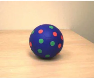
human errors could cause incorrect matches in the tracking process. Figure 1 shows the ball with the stickers applied to the random dot locations.

Figure 1: Marked sphere to be tracked

In addition to the dot locations, the tracking process also requires knowledge of the angle between each unique pair of points (through the center of the sphere). Equation 1 was used to compute the angle for each of the 496 pairs, and the angles were stored in a sorted list.

2.1

Sphere location

Locating the sphere in a scene from the real-time video stream is a two step process. First, the location of the perspective sphere projection on the image plane is found in the current frame. Then, from the projection in pixel coordinates, the 3D location of the sphere in world coordinates is computed using the intrinsic parameters of the camera. We now describe this process in more detail.

Every projection of a sphere onto a plane is an exact circle. This fact, along with the fact that the ball was chosen to be completely one color are the important factors in locating the sphere projection on the image plane. Specifically, the problem is to find a blue circle in the input image. To solve this problem we use the Hue-Saturation-Value (HSV) color space. The hue is the type of color (such as ’red’ or ’blue’), ranging from 0 to 360. The saturation is the vibrancy or purity of the color, ranging from 0 to 100 percent. The lower the saturation of a color, the closer it will appear to be gray. The value refers to the brightness of the color, ranging from 0 to 100 percent. The input image is converted from RGB space to HSV space as follows;

S= ( (V − min(R, G, B))(255 V ) if V > 0 0 otherwise H=      (G − B)(60 S) if V = R 180 + (B − R)(60 S) if V = G 240 + (R − G)(60 S) if V = B (3) The use of HSV space instead of RGB space allows the sphere tracking to work under varying illumination conditions. The image is then binarized using the pre-computed hue value of the blue ball as a target value. The binary image is computed as follows;

Bi=      0 if Ii < T − ǫ 0 if Ii > T + ǫ 1 otherwise (4)

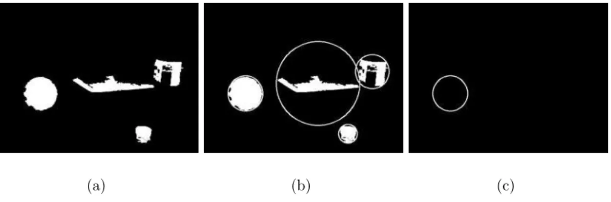
where T is the target hue, and ǫ is a small value to generate an acceptable hue window. In the special case that T − ǫ < 0, the computation for the binary image takes into account the fact that hue values form a circle that wraps around at zero. From the computed binary image, the set of all contours are computed. These first steps are illustrated in Figure 2.

(a) (b) (c)

Figure 2: First steps in locating the perspective sphere projection. a) input image; b) binary image; c) set of all contours.

Since there are many contours found, the next step is to filter out the ones that are not likely to be a projection of a sphere. The process searches for the contour that most closely approximates a circle; so all contours are tested for size and number of vertices. Testing the size of the contours, computed as the pixel area, Ai, occupied by contour i, removes unwanted noise in the image. We decided that a contour must occupy 1500 pixels in order to be processed further. It is then assumed that any circle will contain a minimum number of vertices, in this case, 8. For each contour that

passes the above tests, the minimum enclosing circle with radius ri is found, and then the following ratio is computed;

Ri = Ai

ri

(5) For a circle this ratio Ri is a maximum, therefore the contour that maximizes Ri is chosen as the projection of the sphere onto the image plane, since that contour most closely represents a circle. Figure 3 illustrates the remaining steps to find this projection, continuing from Figure 2.

(a) (b) (c)

Figure 3: Final steps in locating the perspective sphere projection. a) filtered con-tours; b) minimum enclosing circles; c) most circular contour (chosen to be the pro-jection of the sphere).

If the perspective projection of the sphere was found in the input image, processing continues to the second step in locating the sphere, which is to calculate its 3D location in the scene. The scene is a 3D coordinate system with the camera at the origin. Assuming that the intrinsic parameters of the camera are known in advance, namely the focal length and principal point, the location of the sphere is computed from its perspective projection using the method of [6]. Consider the top-down view of the scene in Figure 4, where the focal length of the camera is f and the principal point is (px, py). If the perspective projection of a point P = (X, Y, Z) in space lies at pixel (u, v) on the image plane then;

u− px fx = X −Z X = −Z(u − px) f (6) Similarly; Y = −Z(v − py) f (7)

Figure 4: Perspective projection of a 3D point

So we have X and Y expressed in terms of the single unknown value Z. For the case of the sphere, the point P can be taken as the center in world coordinates, and then the problem is to find the value of Z for this point. In [6], a new method to solve for Zwas developed based on weak perspective projection, which assumes that the sphere will always be moderately far from the image plane. In this case, the projection of the sphere with radius R is a circle centered on (ui, vi) with radius r. Figure 5 illustrates the scenario. Let Pj be a point on the surface of the sphere that projects to (uj, vj) on the circumference of the projected circle. Now, directly from [6], the radius of the circle on the image plane can be expressed as;

r2 = (uj− ui) 2

+ (vj− vi) 2

(8) Similarly for the sphere;

R2 = (Xj− X) 2 + (Yj− Y) 2 + (Zj − Z) 2 (9) Substituting Equation 6 and Equation 7 into Equation 9 and taking into account that X and Y are both zero, we have;

R2 = (−Zj(uj− ui) f ) 2 + (−Zj(vj− vi) f ) 2 + (Zj− Z) 2 (10) Now, from the weak perspective assumption, Zj = Z. This, and Equation 8 gives;

R2 = (−Z f ) 2 ((uj− ui) 2 + (vj − vi) 2 ) = (−Zr f ) 2 (11)

Figure 5: Weak perspective projection of a sphere And finally;

Z= −Rf

r (12)

Now Equation 12 can be used in conjunction with Equation 6 and Equation 7 to find the 3D location of the sphere in the scene, given the current center, (u, v), and the radius, r, of the perspective projection.

2.2

Sphere orientation

Computing the 3 DOF orientation of the sphere in the scene is a geometric problem that makes use of the green and red dots on the surface of the sphere. The process to compute the orientation is outlined as follows:

1. Locate the projections of the red and green dots on the image plane.

2. Compute the relative polar coordinates of the dots, assuming that the center of projection is the north pole.

3. Choose the two dots that are closest to the center of projection and compute the angle between them (through the center of the sphere).

4. Use the sorted list of pairs to find a set of candidate matches to the two chosen dots.

5. For each pair, orient the virtual sphere to align the two chosen dots and compute a score based on how well all the dots align.

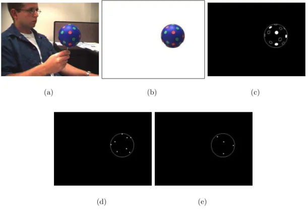
The projections of the green and red dots are located using hue segmentation to binarize the input image. The difference here is that we can restrict the search space to only the part of the input image that is inside the projection of the sphere. Another difference is that the contours retrieved are not expected to be circles but rather ellipses. Using OpenCV, an ellipse is fit to each contour found and its center location in screen coordinates is computed. Figure 6 illustrates the process of locating the dots on the ball surface.

(a) (b) (c)

(d) (e)

Figure 6: Locating the projections of the dots on the sphere. a) input image; b) restricted input; c) ellipses found for the red (filled) and green (un-filled) dots; d) exact green dot locations; e) exact red dot locations.

Once the dots are located, the center of the sphere projection is considered to be the north pole of the sphere, with a latitude value of π/2 radians and longitude value of zero. Then the relative polar coordinates of the projected dots are computed. Let the center of the sphere projection be (uc, vc), the projection of dot i be (ui, vi), the point on the circumference of the sphere projection directly below (uc, vc) be

(ub, vb). Notice that uc = ub. Figure 7 illustrates the situation. The distance, A, between (ui, vi) and (uc, vc), and the distance, B, between (ui, vi) and (ub, vb) are computed easily. The distance between (uc, vc) and (ub, vb) is simply the radius of the circle, r. Since we assume the projection is a top down view of the sphere with

Figure 7: Computing relative polar coordinates

the north pole at the center of the circle, the relative longitude, loni, of dot i is the angle b, which can be computed by a direct application of the cosine rule;

loni = b = cos−1( A2

+ r2 − B2

2Ar ) (13)

Note that if ui < uc, then loni is negative. The calculation for the relative latitude, lati, is simply;

lati= −cos−1( A

r ) (14)

Each dot that was found in the input image (whether red or green) now contains polar coordinates relative to an imaginary north pole at the center of the projection. The next step is to choose the two dots that are closest to the center (i.e. the two that contain latitude values closest to π/2 radians) and compute the angle, θ, between them using Equation 1. This angle is then used to find a set of pairs from the pre-computed sorted list of all possible pairs of dots. The set of possible pairs is the set S, such that the angle between each pair P ∈ S is within a small constant value, ǫ, of θ, and also such that the dot colors match up to the two chosen dots. Each candidate pair is then tested to see how well that pair supports the two chosen dots. The pair with the most support is chosen as the matching pair. The original set of dot locations in polar coordinates can be thought of as a virtual sphere in a standard orientation. The process to test a candidate pair rotates the virtual sphere in order to line up the two points of the pair with the two chosen points in the projection on the image plane. Remember that the two chosen points are on an imaginary sphere with

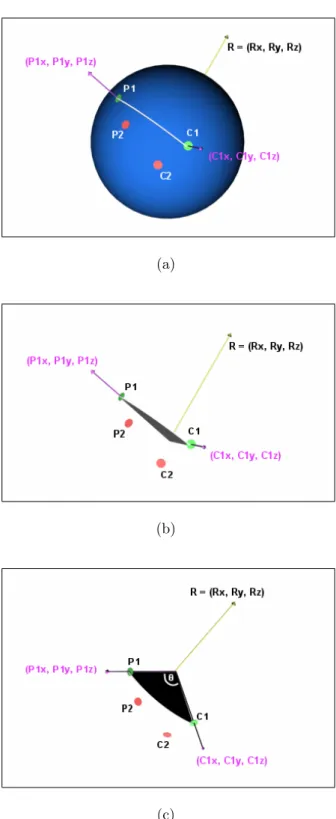
the north pole at the center of projection. The rotation is accomplished in two steps. First, the virtual sphere is rotated about an axis perpendicular to the plane formed by the first point in the pair, the first chosen point and the center of the sphere. This rotation, illustrated in Figure 8, aligns the first point. Then, the virtual sphere is rotated about the vector connecting the center of the sphere to the first point in order to align the second point, as illustrated in Figure 9. Note that in Figure 8 and Figure 9, the first point is shown in green and the second point is shown in red to facilitate distinction. However, any combination of green-red, red-green, green-green or red-red is possible for the two chosen points. In the case of green-green and red-red, the rotation and testing process is repeated a second time after switching the first point and the second point. To explain Figure 8 in more detail, assume the chosen points are C1 and C2, and the points of the stored pair are P1 and P2. Unit vectors (P1x, P1y, P1z) through P1 and (C1x, C1y, C1z) through C1 are computed, using the following conversion from polar to Cartesian coordinates;

X = cos(lat)sin(lon) Y = sin(lat)

Z = cos(lat)cos(lon)

(15)

The axis of rotation, R, to align P1 and C1 is computed from the cross product of the two unit vectors. The angle of rotation is θ, which is the known angle between the two dots. To explain Figure 9 in more detail, P1 and P2 have been rotated to become P1′ _{and P2}′_{, respectively. Now, P1}′ _{and C1 are aligned, and the new axis} of rotation, R, to align P2′ _{and C2 is the unit vector (C1}

x, C1y, C1z) through P1′ and C1. Unit vectors through C2 and P2′ _{are computed using Equation 15. To} compute the angle of rotation, θ, let the vector u = (ux, uy, uz) be the projection of (C2x, C2y, C2z) onto R, and the vector v = (vx, vy, vz) be the projection of (P2x′, P2y′, P2z′) onto R. Then, manipulating the dot product we have;

|u||v|cos(θ) = (uxvx) + (uyvy) + (uzvz) θ = cos−1₍(uxvx) + (uyvy) + (uzvz)

|u||v| ) (16)

This rotation aligns the second point. The one item that has yet to be described is how the virtual sphere is actually rotated by an arbitrary angle, θ, about an arbitrary axis, R = (Rx, Ry, Rz). The sphere is rotated by rotating the unit vectors that correspond to each of the dots on the sphere surface, one at a time. To rotate a unit vector vi = (x, y, z), the entire space is first rotated about the X-axis to put R in the XZ plane. Then the space is rotated about the Y-axis to align R with the Z-axis. Then the rotation of vi by θ is performed about the Z-axis, and then the inverse

of the previous rotations are performed to return to normal space. This can all be accomplished by multiplying each unit vector vi by the following rotation matrix;



 

cos(θ) + (1 − cos(θ))Rx 2

(1 − cos(θ))RxRy− Rzsin(θ) (1 − cos(θ))RxRz+ Rysin(θ) (1 − cos(θ))RxRy + Rzsin(θ) cos(θ) + (1 − cos(θ))Ry

2

(1 − cos(θ))RyRz− Rxsin(θ) (1 − cos(θ))RxRz− Rysin(θ) (1 − cos(θ))RyRz+ Rxsin(θ) cos(θ) + (1 − cos(θ))Rz

2



 

Once the virtual sphere is aligned to the two chosen points, a score is computed for this possible orientation. The validity of a given orientation is evaluated based on the number of visible dots in the perspective projection that align to real dots of the correct color on the virtual sphere, as well as how closely the dots align. Visible dots that do not align to real dots decrease the score, as do real dots that were not matched to visible dots. All points are compared using their polar coordinates, and scores are computed differently based on the latitude values of the points, since points that are closer to the center of the sphere projection should contain a smaller error than those that are farther from the center. Two points, P1 and C1, are said to match if the angle, θ, between them satisfies the following inequality;

θ < (1 + latc1· 2

π)(α − β) + β (17)

where α is a high angle threshold for points that are farthest from the center of pro-jection, and β is a low angle threshold for points that are at the center of projection. In our experiments, values of α = 0.4 radians and β = 0.2 radians produces good results. Using Equation 17, the number of matched dots is calculated as Nm for a given orientation. Let Nv be the number of visible dots that are not aligned to real dots, let Nr be the number of real dots that are not matched with visible dots (and yet should have been), and let θi be the angle between the matching pair, i. Then the score, σ, is computed as follows;

σ = PNm i=1 h (1 + lati· 2 π)(α − β) + β − θi i − PNv i=1 h (1 + lati· 2 π)(α − β) + β i − PNr i=1 h α − (1 + lati· 2 π)(α − β) i (18)

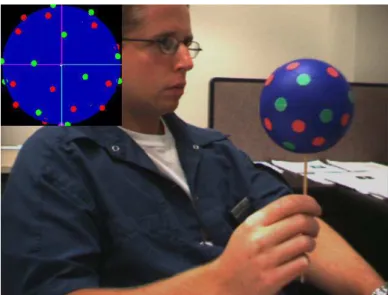
The orientation that yields the highest score is chosen as the matching orientation for the sphere in the scene. Figure 10 shows a screenshot of the sphere in an arbitrary orientation with the matching orientation of the virtual sphere shown in the upper left corner.

3

Occlusion handling

One of the main benefits of our sphere tracking method is that the tracking does not fail during partial occlusions. Occlusion is when an object cannot be completely

seen by the camera. This normally results from another object coming in between that object and the camera, blocking the view. Section 2.1 explains that the tracking method chooses the best-fit circle of the correct hue in the projection of the scene as the location of the sphere. This means that objects can partially occlude the sphere and yet it may still be chosen as the best-approximated circle. Also, since the minimum enclosing circle is computed from the contour, only the pixels representing 180 degrees of the circumference plus one pixel are required in order to determine the location of the sphere with the correct radius. For this reason, up to half of the sphere projection may be occluded and yet its 3D location will still be computed correctly. Furthermore, the tracking process does not require that all of the dots on the surface of the sphere be visible in order to determine the orientation of the sphere. Since the matched orientation with the best score is chosen, it is possible to occlude a small number of the dots and yet still track the orientation correctly. The ability to correctly handle partial occlusions is very beneficial in a sphere tracking process because it allows a person to pick up the sphere and manipulate it with their hands. Figure 11 shows how the sphere tracking does not fail under partial occlusion. In this screenshot, the sphere is used in an augmented reality application where a red teapot is being augmented at the location and orientation of the sphere in the scene.

4

Error analysis

The purpose of this section is to determine the accuracy of the sphere tracking method that we present. Locating the 3D position of the sphere is not a new technique, however the novelty of this paper lies in the algorithm to determine the 3D orientation of the sphere. Therefore, we will only analyze the performance of that algorithm.

In order to compute an error on the resulting 3D orientation calculation of our tracking method, the sphere must be manually placed in the scene with a known orientation. This is a very difficult task because the sphere is a physical object and it is nearly impossible to determine its actual orientation in the scene before performing the tracking. For this reason, a virtual 3D model of the sphere was built with exact precision. Then the virtual sphere model was rendered into the scene at a chosen orientation, and the tracking procedure was applied. The actual orientation and the tracked orientation were then compared to determine a tracking error. Specifically, 100000 video frames were captured with the virtual sphere inserted at random orien-tations. To avoid additional error due to the weak perspective projection computation described in section 2.1, the virtual sphere was constrained to X and Y values of zero, such that the perspective projection was always in the center of the image plane. The Z value of the sphere was chosen randomly to simulate different distances from the camera. The question that remains is how can one 3D orientation be compared to

another? It was decided that a particular orientation of the sphere would be defined by the quaternion rotation that transformed the sphere from its standard orientation. A quaternion is a 3D rotation about a unit vector by a specific angle, defined by four parameters (three for the vector and one for the angle). The two orientations were compared by analyzing the two quaternions. This produced two errors, one error on the quaternion axis and one in the angle. The axis error was computed as the distance between the end points of the two unit vectors which define the quaternions. The angle error was simply the difference between the two scalar angle values. So for each of the 100000 chosen orientations we have a 6-dimensional vector (4 dimensions for the quaternion and 2 for the errors) to describe the tracking error. Visualizing the error for analysis is a non-trivial task. Even if the errors are analyzed separately, it is still difficult to visualize two 5 dimensional vectors. However, we realize that the results of the error analysis will indicate how well the tracking method is able to determine the best match to the perspective projection of the dots on the surface of the sphere. This, in turn, will give some feedback on how well the dots were placed on the sphere and could indicate locations (in polar coordinates) where the dots were not placed well. So instead of visualizing all four dimensions of a quaternion, the polar coordinates of the center of the perspective projection were computed for each orientation. This assumes that a perspective projection of the sphere under any 2D rotation will yield similar errors, which is a reasonable assumption. Now the errors can be analyzed separately as two 3 dimensional vectors (2 dimensions for the polar coordinates and one for the error). Figure 12 is a graph of the average error in the quaternion axis over all the polar coordinates, and Figure 13 is a similar graph of the average error in quaternion angle. In both graphs, darker points indicate greater error and white points indicate virtually no error. It is clear to see from Figure 12 that the greatest error in quaternion axis is concentrated around the latitude value of −π radians, that is to say, the north pole of the sphere. Figure 13 indicates that the error in quaternion angle is relatively uniform across the surface of the sphere. Addition-ally, the overall average error in quaternion axis is 0.034, and in quaternion angle is 0.021 radians. This analysis shows that the sphere tracking method presented in this paper has excellent accuracy. These results were obtained on a Pentium 3 processor at 800Mhz using a color Point Grey Dragonfly camera with a resolution of 640x480 pixels.

5

Future work

There are a few drawbacks with our sphere tracking method that could benefit from future research. The first problem is with locating the perspective projection of the sphere on the image plane. Segmenting the input image by hue value allows

continuous tracking under variable lighting conditions. However, if the projection of another object with the same hue as the blue ball overlaps the projection of the ball then the contours of the two objects will merge into a single connected component. This produces an awkward shape in the binary image and tracking will fail. One solution to this problem is to segment the input image using standard edge detection techniques and then decide which contour most closely represents the sphere, even under partial occlusions.

Another problem with the method presented in this paper is that the locations of the dots on the surface of the sphere were generated randomly and then measured out and placed on the ball by hand. This technique is prone to human error which would lead to errors in the tracking process. A better solution would be to place the dots on the ball first, such that one can visually decide on the locations in order to maximize the tracking robustness, and then have the system learn the dot locations from the input video.

The final drawback presents the most interesting problem to be solved by future research. The problem is that since the dot locations were generated randomly there is no way to guarantee that the perspective projection of two different sphere orien-tations are significantly different. If the projection of two different orienorien-tations are similar then tracking errors will occur. So the question becomes, how can N locations be chosen on the surface of a unit sphere such that the perspective projection of the sphere is maximally unique from every viewpoint? However, in practice this situation is rare.

6

Results and applications

We have presented a method to track the 3d position and orientation of a sphere from a real-time video stream. The sphere is a simple blue ball with 32 randomly placed green and red dots. Tracking consists of locating the perspective projection of the sphere on the image plane using standard computer vision techniques, and then using the projections of the dots to determine the sphere orientation using 3D geometry.

Resolving the 6 DOF pose of a sphere in a real-time video sequence can lead to many interactive applications. One application that was hinted at in section 3 is in the field of augmented reality. Augmented reality is the concept of adding virtual objects to the real world. In order to do this, the virtual objects must be properly aligned with the real world from the perspective of the camera. The aligning process typically requires the use of specific markers in the scene that can be tracked in the video, for instance, a 2d pattern on a rigid planar object [1]. An alternate way to align the real world and the virtual objects is to use the marked sphere and tracking method described in this paper. Once the location and orientation of the sphere is

calculated, a virtual object can be augmented into the scene at that position. The equivalent planar pattern method would be to use a marked cube [5]. Figure 14 shows an augmented reality application using both a marked cube and the proposed sphere to augment a virtual sword for an augmented reality video game. The advantage of tracking the sphere over tracking the cube is that the sphere is more robust under partial occlusions, as described in section 3.

A similar application of our sphere tracking method is to use the sphere as an input device for an interactive 3D application. In many fields such as biology, chemistry, architecture, and medicine, users must interactively control 3D objects on a computer screen for visualization purposes. Some systems require a combination of key presses and mouse movements to rotate and translate the objects. This is often a complicated task that requires a learning period for the users. An interactive input device, such as the sphere described in this paper, could aid in these HCI applications. If the pose of the sphere is mapped directly to the orientation of a virtual object on the screen, then the natural handling and rotating of the device would translate into expected handling and rotating of the virtual object.

There is no limit to the number of applications where sphere tracking could provide a benefit. Any computer vision problem that requires knowledge of the pose of real objects from video images could make use of our sphere tracking method.

References

[1] ARToolKit. http://www.hitl.washington.edu/artoolkit.

[2] Gary Bradski. The OpenCV library. Dr. Dobb’s Journal of Software Tools, 25(11):120, 122–125, nov 2000.

[3] Teh-Chuan Chen and Kuo-Liang Chung. An efficient randomized algorithm for detecting circles. Comput. Vis. Image Underst., 83(2):172–191, 2001.

[4] Richard O. Duda and Peter E. Hart. Use of the hough transformation to detect lines and curves in pictures. Commun. ACM, 15(1):11–15, 1972.

[5] Morten Fjeld and Benedikt M. Voegtli. Augmented chemistry: An interactive educational workbench. In IEEE and ACM International Symposium on Mixed

and Augmented Reality (ISMAR 2002), pages 259–260, September 2002.

Darm-stadt, Germany.

[6] Michael Greenspan and Ian Fraser. Tracking a sphere dipole. In 16th

[7] Euijin Kim, Miki Haseyame, and Hideo Kitajima. A new fast and robust circle extraction algorithm. In 15th International Conference on Vision Interface, May 2002. Calgary, Canada.

[8] Robert A. McLaughlin and Michael D. Alder. The hough transform versus the upwrite. IEEE Trans. Pattern Anal. Mach. Intell., 20(4):396–400, 1998.

[9] Gerhard Roth and Martin D. Levine. Extracting geometric primitives. CVGIP:

Image Underst., 58(1):1–22, 1993.

[10] Reza Safaee-Rad, Ivo Tchoukanov, Kenneth Carless Smith, and Bensiyon Ben-habib. Three-dimensional location estimation of circular features for machine vision. Transactions on Robotics and Automation, 8(5):624–640, 1992.

[11] Y.C. Shiu and Shaheen Ahmad. 3d location of circular and spherical features by monocular model-based vision. In IEEE Intl. Conf. Systems, Man, and

Cyber-netics, pages 567–581, 1989.

[12] L. Xu, E. Oja, and P. Kultanen. A new curve detection method: randomized hough transform (rht). Pattern Recogn. Lett., 11(5):331–338, 1990.

[13] H. K. Yuen, J. Illingworth, and J. Kittler. Detecting partially occluded ellipses using the hough transform. Image Vision Comput., 7(1):31–37, 1989.

(a)

(b)

(c)

Figure 8: Rotation to align the first point. a) standard view; b) with sphere removed for visualization; c) rotated view for clarity.

Figure 9: Rotation to align the second point

(a) (b)

(c) (d)

Figure 11: Handling partial occlusions. a) un-occluded input; b) un-occluded track-ing; c) occluded input; d) occluded tracking.

Figure 12: Analysis of error on quaternion axis