Analyzing and Creating Forms: Rapid Generation
of Graphic Statics Solutions through RhinoScript
by
Michael S. Shearer
B.S. Civil and Environmental Engineering
Cornell University, 2009
THE DEPARTMENT OF CIVIL AND ENVIRONMENTAL
PARTIAL FULFILLMENT OF THE REQUIREMENTS FOR
THE DEGREE OF
MASTER OF ENGINEERING IN CIVIL AND ENVIRONMENTAL
ENGINEERING
AT THE
MASSACHUSETTS INSTITUTE OF TECHNOLOGY
JUNE 2010
@2010 Michael S. Shearer. All rights reserved.
The author hereby grants to MIT permission to reproduce
_
and to distribute publicly paper and electronic
copies of this thesis document in whole or in part
in any medium now known or hereafter created.
ARCHNES
ASSACHUSETTS INSTUJTE OF TECHNOLOGYJUL 15 2010
LIBRARIES
Signature of Author ...
....
...
Department of Civil and Environmental Engineering
May 7, 2010
Certified by...
Joh sendorf
Associate Professor of Civil and Environmen al Engineering and Architecture
Thesis Super
r
A ccepted by ...
Daniele Veneziano
Chairman, Departmental Committee for Graduate Students
SUBMITTED TO
Analyzing and Creating Forms: Rapid Generation of
Graphic Statics Solutions through RhinoScript
by
Michael S. Shearer
Submitted to the Department of Civil and Environmental Engineering on May 7, 2010, in partial fulfillment of the
requirements for the degree of
Master of Engineering in Civil and Environmental Engineering
ABSTRACT
Graphic statics is a method of structural analysis which relies solely on geometric constructions to determine axial forces within members. Accordingly, any computer-aided drafting (CAD) program may be utilized in the pursuit of a graphic statics solution. This thesis presents a methodology which employs Rhinoceros 4.0 (Rhino) in its capacity as such a program. Using RhinoScript, which provides access to Visual Basic Scripting, or VBScript, within Rhino, the basic steps of graphic statics are automated as scripts. The scripts are then compiled into RhinoStatics, a plug-in module which facilitates graphic statics analyses.
The thesis focuses on three applications of graphic statics: determination of simply supported reaction forces, funicular form-finding given restraints on the axial capacity of the material being used, and determination of axial forces within a pin-jointed truss loaded at its nodes. While only these three applications are explored in detail, the developed scripts may be used in the pursuit of a wide range of graphical equilibrium solutions, transforming Rhino into a highly specialized tool in the hands of a user with knowledge of graphic statics techniques. Such users will be able to easily analyze a host of two-dimensional cross-sections and forms, as well as generate new shapes given loading and geometric constraints. Users familiar with VBScript could easily expand on the documented script files to add functionality to suit their own needs.
In addition to providing worked examples of how to utilize the RhinoStatics plug-in module, this thesis provides a brief overview of graphic statics plug-in general. The developed scripts are explained in detail, with fully documented RhinoScript code provided in the appendices.
Thesis Supervisor: John Ochsendorf
Acknowledgments
It goes without saying that any major project such as a thesis is not completed in a vacuum, nor solely through the efforts of the author. With that in mind, I would like to thank the following individuals for their contributions to the successful completion of this thesis:
John Ochsendorf for his support, guidance, and encouragement through the entire thesis process. Perhaps most importantly, he introduced me to the concept of graphic statics, a true "twenty-fifth century method" which just happened to be first developed in the eighteenth century. Throughout the development of the RhinoStatics plug-in, he was an invaluable sounding board, always looking to possible future applications and trying to push the project as far as it would go. It has been a privilege to have him as my advisor, and I look forward to future collaborations.
Patrick McCafferty (Arup) for recommending John as a thesis advisor and for challenging me to develop my project into something truly original. Pat first suggested expanding the thesis from a series of case studies into a full-fledged program capable of performing graphic statics. Without his influence, this whole project would have looked very different, and with his continued influence, it may evolve even further.
Tom Chatt (Cornell University, ECE MEng 2010) for helping me though my largest programming endeavor to date and for providing support even after the scripting was complete. From I4TEX assistance to proofreading of the final draft, I am indebted to Tommy for the high quality of my finished thesis, both its content and its visual appeal.
My family and friends for their constant love and unflagging support through what have been a grueling nine months. The constant workload and long hours were made easier by having people in my life with whom I could share both the highs and the lows.
The Schoettler Scholarship Fund for providing me with the full tuition scholar-ship which allowed me the freedom to pursue this Master of Engineering degree. Though rigorous and demanding, obtaining this degree has been immensely re-warding.
In pursuing the Master of Engineering degree, I sought to improve myself as an engineer by broadening the tools at my disposal. At the beginning of this program, I had never even heard of graphic statics; however, as my time at MIT draws to a close, I believe learning to harness it may have been the most important skill I gained. For that, I am immensely grateful to everyone who assisted in this endeavor.
This thesis was typeset using the MiKTEX 2.8 implementation of LATEX for Windows and the mitthesis template provided on Athena. TEXnicCenter served as the text editor and compiler.
Contents
1 Introduction
1.1 Problem Statement . . . . 1.2 Literature Review . . . . 1.3 RhinoStatics . . . . 2 Review of Graphic Statics Methodology
2.1 Definitions . . . . 2.2 Bow's Notation . . . . 2.3 Load Line Construction . . . . 2.4 Simply Supported Reactions . . . . 2.5 Force and Funicular Polygons . . . .
2.5.1 Funicular Shapes 2.5.2 Truss Analysis . 3 RhinoScript Programming 3.1 Why Rhinoceros? . . . . 3.2 Script-Level Routines 3.2.1 GetLoadScale 3.2.2 GetPlane . . . . 3.2.3 GetBowsSize 3.2.4 GetForceScale 3.2.5 GetForceSize 3.2.6 GetAxialSize 3.2.7 MakePoint . . . . 3.2.8 MakeLabel . . . . 3.2.9 LabelOverlap 3.2.10 IntersectLines 3.2.11 SlopeVector . . . 3.2.12 MakeParallelLine 3.2.13 DrawPin . . . . . 3.2.14 DrawRoller . . . 3.3 User-Level Routines . . . 3.3.1 AddSupports . . 3.3.2 ApplyLoads . . . 3.3.3 MakeLineOfAction . . . Methodology . . . . . . . . . . . . .
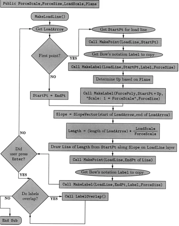
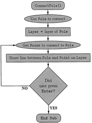
3.3.4 AddBows . . . . . 3.3.5 MakeLoadLine 3.3.6 MakePole . . . . . 3.3.7 ConnectPole . . . . 3.3.8 MakeFunicular 3.3.9 MakeClosingString 3.3.10 CloseLoadLine 3.3.11 MakeForce . . . . . 3.3.12 LabelForcePoly . . 3.3.13 GetForceLabel . . . 3.3.14 ViewGlobals . . . . 3.4 Concluding Thoughts . . . 4 Implementation Examples 4.1 4.2 4.3 4.4
Simply Supported Reaction Forces . . . . . Analysis of Ideal Truss Loaded at Joints . . Form-Finding with Material Restraints . . . Optimization of Truss Under Vertical Loads 5 Conclusion
5.1 Discussion . . . . 5.2 Recommendations for Further Development
5.2.1 Functionality in Any 2D Plane . . . . 5.2.2 Parametric Linkages . . . . 5.2.3 Automated Structural Optimization . 5.2.4 Increased Robustness . . . . 5.2.5 Improved Graphic Interface . . . . . A RhinoScript Code for
A.1 DrawPin . . . . A.2 DrawRoller . . . . A.3 GetAxialSize . . . A.4 GetBowsSize . . . . A.5 GetForceScale . . . A.6 GetForceSize . . . A.7 GetLoadScale . . . A.8 GetPlane . . . . A.9 IntersectLines . . . A.10 LabelOverlap . . . A.11 MakeLabel . . . . . A.12 MakePoint . . . . . A.13 MakeParallelLine . A.14 SlopeVector . . . . Script-Level Routines . . . . . . . . . . . . . . . . . . . . . . . . . . . . . . . . 103 . . . . 104 . . . . 106 . . . . 108 . . . . 109 . . . . 110 . . . . 111 . . . . 112 . . . . 113 . . . . 114 .. .... 118 . . . . 120 . . . . 121 . . . . 122 . . . . 124 . . . 52 . . . 52 52 55 . . . 55 . . . 58 . . . 58 . . . 61 64 . . . 64
B RhinoScript Code for User-Level Routines 125 B.1 AddBows ... . 126 B.2 AddSupports ... ... 130 B.3 ApplyLoads . . . . 137 B.4 CloseLoadLine . . . . 140 B.5 ConnectPole . . . . 146 B.6 GetForceLabel . . . . 147 B.7 LabelForcePoly . . . . 152 B.8 MakeClosingString . . . . 156 B.9 MakeForce . . . . 159 B.10 MakeFunicular . . . . 167 B.11 MakeLineOfAction . . . . 173 B.12 MakeLoadLine . . . . 179 B.13 MakePole . . . . 186 B.14 ViewGlobals . . . . 188
List of Figures
2-1 Sample Bow's notation and associated load line . . . . 2-2 Sample determination of simple support reactions using graphic statics 2-3 Sample determination of funicular arch using graphic statics . . . . . 2-4 Sample determination of axial truss forces using graphic statics . . . . 2-5 Completed determination of axial truss forces using graphic statics . . 3-1 3-2 3-3 3-4 3-5 3-6 3-7 3-8 3-9 3-10 3-11 3-12 3-13 3-14 3-15 3-16 3-17 3-18 3-19 3-20 3-21 3-22 3-23 3-24 3-25 3-26 3-27 3-28 3-29
Identification of elements used in pseudocode flowcharts . Typical control loop for global variables and layers . . . . Script-Level Subroutine - GetLoadScale . . . . Script-Level Subroutine - GetPlane . . . . Script-Level Subroutine - GetBowsSize . . . . Script-Level Subroutine - GetForceScale . . . . Script-Level Subroutine - GetForceSize . . . . Script-Level Subroutine - GetAxialSize . . . . Script-Level Subroutine - MakePoint . . . . Script-Level Subroutine - MakeLabel . . . . Script-Level Subroutine - LabelOverlap. . . . . Script-Level Function - IntersectLines . . . . Script-Level Function - SlopeVector . . . . Script-Level Subroutine - MakeParallelLine . . . . Script-Level Function - DrawPin . . . . Script-Level Function - DrawRoller . . . . User-Level Subroutine - AddSupports . . . . User-Level Subroutine - ApplyLoads . . . . User-Level Subroutine - MakeLineOfAction . . . . User-Level Subroutine - AddBows . . . . User-Level Subroutine - MakeLoadLine . . . . User-Level Subroutine - MakePole . . . . User-Level Subroutine - ConnectPole . . . . User-Level Subroutine - MakeFunicular . . . . User-Level Subroutine - MakeClosingString . . . . User-Level Subroutine - CloseLoadLine . . . . User-Level Subroutine - MakeForce . . . . User-Level Subroutine - LabelForcePoly . . . . User-Level Subroutine - GetForceLabel . . . .
. . . . 32 . . . . 32 . . . . 35 . . . . 35 . . . . 35 . . . . 37 . . . . 37 . . . . 39 . . . . 39 . . . . 39 . . . . 40 . . . . 41 . . . . 43 . . . . 43 . . . . 44 . . . . 44 . . . . 46 . . . . 48 . . . . 49 . . . . 51 . . . . 53 . . . . 54 . . . . 54 . . . . 56 . . . . 57 . . . . 59 . . . . 60 . . . . 62 . . . . 63 3-30 Graphic representation of interdependencies between routines .
4-1 RhinoStatics plug-in implemented into Rhinoceros 4.0 . . . . 67
4-2 Layers resulting from use of RhinoStatics plug-in . . . . 68
4-3 Conceptual sketch for Example 4.1 . . . . 69
4-4 Step-by-step depiction of Example 4.1 . . . . 70
4-5 Completed RhinoStatics solution for Example 4.1 . . . . 75
4-6 Conceptual sketch for Example 4.2 . . . . 76
4-7 Geometry, load arrows, Bow's notation, and completed load line for Exam ple 4.2 . . . . 77
4-8 Completed force polygon for Example 4.2 . . . . 78
4-9 Completed RhinoStatics solution for Example 4.2. . . . .. 79
4-10 Conceptual sketch for Example 4.3 . . . . 80
4-11 Geometry, load arrows, Bow's notation and preliminary load line for Exam ple 4.3 . . . . 81
4-12 Completed Bow's notation and load line for Example 4.3 . . . . 83
4-13 50 kip limiting circle and resulting force polygon for Example 4.3 . . 84
4-14 Funicular shape based on 50 kip tensile limit for Example 4.3 . . . . . 86
4-15 25 kip compressive limit imposed for Example 4.3 . . . . 86
4-16 Funicular shape based on 25 kip compressive limit for Example 4.3 87 4-17 Original truss shape with loads and simple supports shown . . . . 88
4-18 Original truss shape with Bow's notation and load line . . . . 89
4-19 Original truss shape with axial forces shown on both force polygon and shape... ... 90
4-20 Limiting line determined for first iteration of truss shape . . . . 91
4-21 First iteration of force polygon based on limiting line established in Figure 4-20 . . . . 92
4-22 First iteration of truss shape with axial forces shown on both force polygon and funicular shape . . . . 93
4-23 Partial force polygon for second iteration showing determination of limiting line... . . . . . . . . . . . . 94
4-24 Completed second iteration of truss shape with axial forces shown on both force polygon and funicular shape . . . . 94
4-25 Comparison of three truss forms . . . . 94 5-1 Thrust line for existing masonry arch under asymmetrical live loading 96
List of Tables
4.1 Table of menu descriptions and corresponding user-level routines . . . 68 4.2 Table of axial forces for each iteration of truss shape . . . . 90
Chapter 1
Introduction
1.1
Problem Statement
Referring to British engineering practices in the mid-1800s, W. J. Macquorn Rankine, a professor of civil engineering and mechanics at the University of Glasgow, wrote:
... of that scientifically practical skill which produces the greatest effect with the least possible expenditure of material and work, the instances are comparatively rare. In too many cases we see the strength and the stability, which ought to be given by the skilful[sic] arrangement of the parts of a structure, supplied by means of clumsy massiveness, and of lavish expenditure of material, labour, and money...
- A Manual of Applied Mechanics[9] (1858)
Though written over 150 years ago, Rankine's sentiment still applies today. There is virtually no end to the powerful computer analysis programs currently available to structural engineers, allowing for the rapid determination of member forces under a multitude of loading combinations. By harnessing this analytical power, member sizes may be optimized and stiffnesses perfected to bring to fruition almost any ge-ometric configuration with relatively little effort. In doing so, this computational power is harnessed towards what Rankine called "clumsy massiveness, and... lavish expenditure of material, labour, and money," rather than the generation of a form which "produces the greatest effect with the least possible expenditure of material
and work."
Structural engineers are quick to defend their profession as more than just sizing beams and columns, so one must wonder why the bulk of their computational effort is expended toward this end. In many cases, a more appropriate expenditure of computational effort and time would be assisting in the creation of a more efficient form, rather than enabling inefficient forms through excessive material usage. The problem, then, becomes one of developing a computational tool which allows engineers to assist architects in developing shapes which derive strength and stiffness from the geometric configuration of their elements, rather than simply the geometric and
material properties of those elements. Ideally, such a tool would also be accessible directly to the architects so that they might become equal partners in this design approach.
Fundamentally, such a method already exists: graphic statics. Graphic statics allows for the solution of statics problems through purely geometrical constructions, relying on scale drawings and parallel lines to determine the forces within members. The method is not a new one; originally executed on drafting tables by engineers wielding t-squares and triangles, it arguably predates the first numerical methods of structural analysis.1 Given the age of the technique, it becomes obvious that the goal in de-veloping an appropriate computational tool lies not in perfecting a method, but in making that method readily available to designers in a format which is compatible with the computerized state of the profession.
1.2
Literature Review
ActiveStatics
Developed by Simon Greenwold at the Massachusetts Institute of Technology, Act-iveStatics[6] represents the first computer implementation of graphic statics. The program provides a number of dynamically linked examples of graphic statics so-lutions. Axial forces within members are represented by colors, indicating either tension, compression, or zero force, and by lines drawn with width proportional to magnitude. A very powerful teaching tool, ActiveStatics does not provide meaningful design capabilities, unless the user happens to be designing one of the provided forms under an identical load case.
StaticsPad
As a follow-up to ActiveStatics, Greenwold is currently developing StaticsPad[7], which extends the concept of ActiveStatics to allow users to generate their own shapes. A work in progress, StaticsPad will ultimately allow the creation of parametrically linked funicular and force polygons - moving a node on either polygon will affect both. As with ActiveStatics, axial forces' sense and magnitude will be represented by color and line thickness, respectively, on both polygons. Where ActiveStatics is only a tool for understanding graphic statics, StaticsPad will be a tool for harnessing the ability of graphic statics to generate and optimize axial structures. The positions of nodes are readily accessible on a x-y coordinate system, but the functionality of
'The concept of paired force and funicular polygons, the cornerstone of graphic statics, was first published by Varignon in 1725. Poleni used graphical methods to analyze St. Peter's Basilica in 1748. Louis Navier first laid the groundwork for modern numerical methods in a text published in 1826, some 78 years later. While others published graphical methods of truss analysis in the mid-1800s, the generally acknowledged father of graphic statics is Karl Culmann, who published Die graphische Statik in 1866.[1]
exporting whole models directly has not appeared at this point in the development process.
InteractiveTHRUST
Developed by Philippe Block as part of his Master of Architecture thesis[2] at the Massachusetts Institute of Technology, InteractiveTHRUST[3] provides an analysis tool which examines the thrust lines of vaulted masonry structures through graphic statics. Connected parametrically to a force polygon, these thrust lines can be used to determine forces and potential collapse modes for the masonry structures. The geometry of individual arch segments provide self-weight loading, allowing for quick and accurate modeling of self-weight conditions for existing and proposed masonry structures. While InteractiveTHRUST provides a very powerful tool for masonry design, by the nature of its limited scope, it is a limited design tool for general practice.
CADenary
Developed by Axel Kilian at the Massachusetts Institute of Techonology, CADenary[8] uses a particle and spring system, rather than graphic statics, to model hanging chains and meshes. Funicular forms under self-weight can be determined using this program, which allows users to specify the number and length of links in the chains. While it promotes the creation of funicular forms, CADenary lacks the ability to analyze the forces within these shapes, and is limited to strictly cable-based forms. Once created, CADenary does allows shapes to be output as .dxf files, allowing a level of interaction with "traditional" programs such as AutoCAD. This functionality is lacking in the programs of Greenwold and Block.
1.3
RhinoStatics
RhinoStatics, the plug-in created for this thesis project, approaches the problem of computerizing graphic statics with a slightly different focus than the previously dis-cussed endeavors. While not parametric like Greenwold's programs, RhinoStatics, by virtue of being a plug-in to the widely used Rhinoceros 3D modeling/drafting software, is directly accessible to both architects and engineers involved in the de-sign process. While certainly suitable as a teaching tool for learning graphic statics, RhinoStatics also has merit as a tool to be used in practice by engineers perform-ing back-of-the-envelope type calculations on forms drawn in Rhino by an architect. In addition to simply analyzing forms, RhinoStatics allows for the rapid generation of funicular forms, be they arches, cable structures, or other statically-determinant forms such as trusses. In addition to promoting efficient design by making available the graphic statics method, by virtue of functioning within Rhino, RhinoStatics al-lows such designs to be easily incorporated into an existing model, exported to other
drafting software, or sent directly to analysis packages for more rigorous testing and refining of the generated form.
Chapter 2
Review of Graphic Statics
Methodology
As general conditions of determining either forms or forces through graphic statics, it is important to remember that solutions are only valid if the structure in question is statically determinant and carries forces in a purely axial manner. Statically in-determinant structures cannot be analyzed because graphic statics does not model the relative stiffnesses of elements, which must be considered to solve problems which are statically indeterminant in nature. Similarly, bending within members is not represented in this method, so only purely axial solutions are possible. A final re-quirement is that all forces and members must be co-planar; graphic statics produces two-dimensional results only. The most common applications of graphic statics are fu-nicular shapes (§2.5.1) and ideal trusses (§2.5.2). Graphic statics can also be utilized to determine the support reactions for simply supported structures (§2.4).
2.1
Definitions
To facilitate clear discussion of the mechanics of graphic statics, it is useful to establish working definitions of a few terms which represent characteristics of vectors.
Direction - The angle which describes a vector's orientation in space, taken coun-terclockwise relative to the horizontal.
Line of action - An infinite line which passes through a vector's point of applica-tion and shares its direcapplica-tion.
Magnitude - The length of a vector.
Point of application - The point at which the load or force represented by a vector is said to act.
Sense - An indicator of the starting and ending points of the vector. May be shown by arrowhead or the notation used to describe the vector. When referring to an axial force, indicates either tension or compression.
AB BC C
B
b ca
A C
CA a
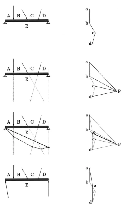
Figure 2-1: Sample Bow's notation and associated load line
2.2
Bow's Notation
Successful execution of graphic statics relies on two basic actions: careful creation of parallel lines and consistent application of Bow's notation. The construction of parallel lines is assumed to be trivial for this discussion. When attempting graphic statics by hand, the task may be accomplished using a ruler and drafting triangle, and when utilizing the plug-in presented later in this paper, the task is fully auto-mated. Bow's notation, however, requires active attention from the user, particularly when determining the sense of axial forces. For that reason, a brief discussion of the mechanics of Bow's notation is prudent.
First published in 18731, Bow's notation is a method of labeling free-body diagrams. Starting at any arbitrary point, one applies a capital letter between each line of action, working clockwise from the starting notation. Bow's notation beings at A, and by convention does not use the letter P, which is reserved for labeling poles. Vectors are then named by the two letters between which their lines of action lie. By convention, capital letters are used for labeling the free-body diagram and lowercase letters are used for the force polygon. For a simple example of Bow's notation applied to a free-body diagram, refer to the left-hand portion of Figure 2-1.
2.3
Load Line Construction
The load line is a particular type of force polygon which includes only forces which are external to the structure being analyzed. Since only applied loads and support reactions are included, the load line may be built without any knowledge of the structural form, requiring only the geometry of the loading and supports. The load line is constructed by placing the load vectors such that they intersect at points corresponding to shared Bow's notation. It is important to note both the line of action and sense of the load vectors when creating the load line. The load line element corresponding to a given load arrow should start at the point labeled with the Bow's notation found counterclockwise from the arrow and end at the point labeled with the clockwise notation.
1Robert Bow,
The following example refers to Figure 2-1. In constructing the load line, the first load vector to be considered is AB, found in the upper left of the free-body diagram. The point a is placed arbitrarily to begin the load line. Next, a line parallel to AB's line of action is drawn such that point b is the same direction relative to point a as the head of the arrow is from the tail. One must establish a scale for the load line (for example, 1 inch = 100 pounds of force). This scale is used in determining the length of the line in the load vector, which must match the scaled magnitude of the force being represented. The next vector to be considered is BC, found in the upper right of the free-body diagram. Its corresponding load line element starts at point b and similarly follows the line of action and direction for a scaled distance, terminating at point c. The final component of the free-body diagram is vector CA. One will observe that both points c and a already appear on the load line. One will also observe that a line from c to a falls along the line of action of vector CA. The length of this line gives the magnitude of vector CA required to place the free-body diagram in equilibrium.
Equilibrium is defined in statics as the simultaneous solution of three equations: EF = 0, EFy = 0, and EM = 0. These equations represent the condition wherein all vector components in the x direction sum to zero, all vector components in the y direction sum to zero, and all moments about a given point sum to zero. In graphic statics, these three conditions are proven to be satisfied if the load line starts and ends at the same point, or "closes." In addition to providing a simple method of confirming equilibrium, this property can be used to determine unknown support reactions, but only in the simply supported case (one pin and one roller). If a system has more supports than these two, graphic statics can still be used to analyze it, but support reactions must be solved using another method, such as the equations above or through analysis software.
Further examples of load lines can be found in Figures 2-2, 2-3, and 2-4.
2.4
Simply Supported Reactions
Though presented as a solution to the particular example found in Figure 2-2, the following methodology can be used to determine simply supported reactions in the general case.
Given a beam which is simply supported (one roller and one pin) with loading of known lines of action, magnitude, and sense, the unknown support reactions may be found. Figure 2-2 shows an example of such a beam. In the first row, Bow's notation has already been applied, and a partial load line has been constructed. Note that the load line does not close, indicating that the system is not in equilibrium based on the forces currently applied. This lack of equilibrium makes sense, given that the support reactions are not represented. The reader will notice the letter E is shown as part of Bow's notation, but not reflected in the load line. This E is anticipating that there will be force vectors at each support, so there must be a notation made to separate
~AB\C/D(
E
*A
B\
c/D
a
b
Cd
E
Ag B
CD
V.
b
E
e
d~
a.
A
B
C
D
E
b
E
d
the lines of action for these two forces (see §2.2).
In the second row, the lines of action for the applied loads have been extended (shown as dashed lines). The line of action for the roller has also been drawn, since it is known to act only up and down in the plane of the image, by the definition of a roller. These lines of action will aid in the creation of a funicular polygon. The second step in preparing to create this funicular polygon is the selection of an arbitrary point on the force polygon, of which the load line is part. This arbitrary pole is labeled with the letter p in the figure. It should be stressed that the location of this pole has no influence on the outcome, as long as it does not lie on the load line itself.
In the third row, the funicular polygon has been drawn and closed with the closing string, which is then used to determine the magnitude and direction of the support reactions. To construct the funicular polygon, one begins at the location of the pin support, since the only thing known about the force at that support is that its point of application lies at the pin. Next, a line parallel to the line ap (from the force polygon) is drawn from the pin until it intersects the line of action for force AB. This intersection point is shown in the figure as a circle. Working clockwise, the next Bow's notation is B, so one draws a line parallel to bp until intersecting the line of action for BC. This process is continued until the last line connecting the load line to the arbitrary pole has been incorporated. This last line (in this case, dp) is terminated at its intersection with the roller's line of action. Once the funicular polygon has been created, a line is drawn from the ending point (the intersection of the last line and the roller's line of action) back to the starting point (the point of application of the pin). This line is called the "closing string." A line parallel to the closing string is then drawn on the force polygon, starting at the arbitrary pole, p. In the figure, the closing string is shown as a bold line.
To determine the support reactions, recall that the line of action of the roller is strictly vertical. Based on Bow's notation, the name of this reaction force will be DE. From this naming convention, it follows that the representation of the roller's reaction in the load line must have one end at the point labeled d. Further, since the load vector for the roller will fall along its line of action, one can trace a line parallel to the line of action (i.e. vertical) from point d until it intersects the closing string. This intersection is labeled with a lowercase e, again based on Bow's notation. Referring once again to Bow's notation, the reaction force at the pin is named EA. Given that points e and a both exist on the load line, it is trivial to connect the two points and find the line of action for the pin's force. Both lines of action are shown in the figure as dashed lines on the force polygon.
In the fourth row, the pole, associated lines, and funicular polygon, having served their purpose, have been removed. On the load line, points d and e have been connected, as have points e and a. From the length and orientation of these points, the reaction forces have been found. Though the senses of these forces seem trivial, it is worth explaining the methodology used in determining them, as it is based on Bow's notation and useful in interpreting all graphic statics results. At the roller, the force
DE has the letter D as its counterclockwise notation, and E as its clockwise notation. Referring to the force polygon, one reads the vector as starting at the counterclockwise notation (in this case, d) and ending at the clockwise notation (e). As such, one can determine that the sense of the roller's reaction is upward, as represented by the arrowhead. Similarly, reading the load line from e to a shows the sense of the pin's reaction, again represented by the arrowhead.
2.5
Force and Funicular Polygons
The force and funicular polygons are related by Bow's notation and lines of action, and represent the axial force and geometry of the structure in question, respectively. Though always related in this way, which polygon "leads" depends on what task is being accomplished. When determining funicular shapes or reaction forces, the force polygon leads; the funicular polygon follows, drawn on the sketch containing the uppercase Bow's notation. In the case of existing structures, such as trusses, the existing geometry serves as the funicular polygon. The force polygon follows this funicular polygon and is labeled with lowercase Bow's notation. The two polygons are related by the fact that lines labeled with corresponding Bow's notation (e.g. AB on the funicular polygon and ab on the force polygon) must have the same line of action. The load line, discussed in §2.3, is a particular subset of the force polygon, and serves as the basis for constructing a full force polygon. Drawn to a particular scale, the force polygon determines axial forces within elements which correspond to the shape set out by the funicular polygon.
The following examples will demonstrate basic techniques of graphic statics which may be used in the pursuit of a wide range of other solutions.2
2.5.1
Funicular Shapes
As a worked example, the case of an arch developed for non-symmetrical loading is considered. The geometry, loading, and material strength are provided, and the funicular shape will be determined. Figure 2-3 displays the graphical steps taken as part of this example.
The arch is to be simply supported, with a pin on the left and a roller four units to the right. Evenly spaced between these two supports are three forces: the first two are one unit of force and the third is two units of force. The reaction forces could be found graphically, or through another numerical method: 1.75 units of force at the pin and 2.25 units of force at the roller. In the first row of the figure, all external forces are represented on the geometry sketch, Bow's notation has been applied, and a load line is constructed at 1:1 scale.
2
For many more applications of graphic statics, the reader is directed to Sondericker's Graphic
Statics[11] (1903), Wolfe's Graphical Analysis[12] (1921), or, more recently published, Allen and
A
B
C
D
A
B
C
D
E....
a
p e.dz
Cl.To establish a funicular shape for the given loading, one must first specify material constraints on the elements which will comprise the shape. Typically, such material constraints are expressed in terms of a maximum allowable stress in the cross section. Such a constraint can easily be converted into a maximum allowable axial force. For this example, such a conversion is assumed to have been performed, resulting in a maximum axial compressive force of three units. Recalling that the length of the lines of the force polygon relate to the axial forces within corresponding members, this constraint is realized graphically as circles with a radius of three units of force, with their centers at each point corresponding to a funicular element (in this case, a, b, c, and d). Such circles are shown shaded on the second row of the figure. The area in which all these circles overlap (outlined with a solid line) represents the area in which a pole could be placed such that all lines from the origin points to that pole would result in axial forces less than or equal to the constraint. If no such overlap exists, then the material constraints cannot be satisfied, and the material strength must be increased.
To ensure that geometric constraints are also met, this solution space must be further refined. To do so, one can envision that a member will be placed between the two supports. The line of action of this member would be labeled with E in the funicular polygon, and thus must pass through the point e on the force polygon. This line of action is shown as dashed in the second row of the figure. To satisfy both material and geometric constraints, any pole which is to provide a funicular shape must lie both within the overlapping layer and on the dashed line of action. By locating the pole p at the intersection of the boundary line and the line of action, it is ensured that at least one of the elements will be stressed to the material limit, providing efficient use of the structural capacity. If the pole were located inside of the boundary line, all elements would be stressed to less than the maximum force. By locating the pole to the left of the load line, an arch shape is created. For example, if the pole labeled p' were selected, the shape generated would represent a cable in which the axial force in all members was less than three units of force. The rationale used to determine pole placement for arches versus cables will become evident shortly.
Having established an appropriate pole for the force polygon, lines are drawn between the pole and points on the load line representing applied forces, shown in the third row. The lines of action for the forces have also been extended on the geometry sketch (shown as dashed lines). As with creating the funicular polygon for determining sup-port reactions, a line parallel to line pa is drawn starting at the pin and terminating at the intersection of the line of action for force AB. The process is continued for all lines on the force polygon. The last line ends at the point of application for the roller, demonstrating geometric compatibility with the placement of the loads and supports, as ensured by the line of action used in the second row of the figure. The reader will notice that had the pole p' been used, line ap' would result in a funicular shape directed down (a cable) rather than the upward direction (an arch) which is demonstrated here.
In the fourth row, the length of each line in the force polygon has been determined, indicating the amount of axial force within each segment. The loads in all segments are equal to or less than the prescribed material strength, indicating a successful design. The reader is directed in particular to the last element, with an axial force of 3.00 units, which resulted from placing the pole on the boundary line. The reader will also notice that the arch "leans" toward the larger force, a good indication that a funicular shape has been derived, rather than the typical arch shape which would result from an even load distribution.
2.5.2
Truss Analysis
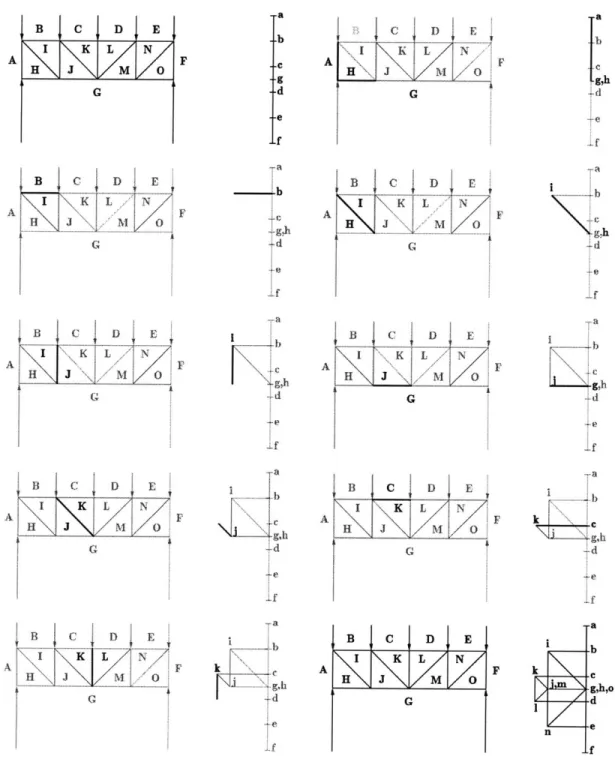
As a worked example, the case of a Pratt truss under symmetrical loading is consid-ered. The truss is considered to be ideal, with all joints pinned and all internal forces purely axial. The truss shape, support conditions, and loading are provided; the force polygon and, consequently, axial forces will be determined. The reader is referred to Figures 2-4 and 2-5, which display the graphical steps taken as part of this example and the final axial forces, respectively. Figure 2-4 is read from right to left, top to bottom.
From symmetric loading of equally spaced unit forces, the reaction forces may be trivially found to be 2.5 units of force each. Once all external forces have been determined, Bow's notation is applied and the load line constructed. The reader will notice that Bow's notation is applied clockwise around the exterior of the truss, then clockwise again through the interior of the truss. This approach ensures that the load line is created with the beginning letters of the notation. Notation in the interior of the truss is such that each member has its own unique identifying combination of Bow's notation.
As mentioned previously, in the case where structural geometry is provided and axial forces are the only unknown, the geometry sketch is taken as the funicular polygon. To fully populate the force polygon, lines parallel to the elements of the funicular polygon are drawn beginning at points which are already labeled on the force polygon. Often, a line of action and point of origin can be determined from one member, but the terminating point cannot be determined without considering another element's line of action. Figure 2-4 graphically demonstrates this process, which will also be explained step-by-step.
The process of building the force polygon begins with identifying a member with one known and one unknown notation. In this case, member AH is chosen because the point a is known on the force polygon, but h is not. A line parallel to the line of action for AH is drawn on the force polygon starting at a. This line conceptually continues infinitely in both directions. The next step is to identify another member with the same unknown (h) and a different known notation, in this case, the member GH. Starting at point g, a line parallel to the member GH is added to the force polygon. At the point where this new line intersects the line drawn for AH, the point h must exist to satisfy both lines ah and gh. In this case, the reader will observe that
B IC I D 11 E \ \K LN H J M 0 a b C g~h -d -e If -d i f F 0 B C DIE \H H J
~M
A [ g,h (-A f B C D E \I K L N I 0F G -d +eB8
Ce
DI K KL N' \TY.i F k H4 3<I1" .... ... ... ... ... .... ... ... ... ... .... ... ... .. ... ... .... . .... ... ... ... C D E H 0 B C D E AF G B C D E I \K L N F H C M 0 GFigure
2-4:
Sample determination of axial truss forces using graphic statics
-a -b g,h Lb ,h d if g,h If k h4 g.h -d
the points g and h must coincide to satisfy this condition. This result indicates that the member GH is a zero-force member, which one could also conclude by inspection of the truss geometry and loading conditions.
Next, the member BI is considered. Since point b is known, a line parallel to BI is drawn starting at b on the force polygon. Point i is not known, so the line is left without an intersection, and one looks for another member whose notation contains both the letter i and a letter whose point is on the force polygon. HI is such a member. Drawing a line parallel to member HI starting at point h, one will intersect the previously drawn line. This intersection is labeled with the letter i, thus generating lines bi and hi on the force polygon. Figure 2-4 shows the continuation of this process until such a point is reached that the remaining force polygon may be generated through symmetry.
Once the force polygon has been completed, it can be used to determine the magnitude and sense of the axial forces within the truss. The reader is referred to Figure 2-5 for the following discussion. Recalling that the force polygon is drawn to the scale of 1 unit of length = 1 unit of force, the length of lines can easily be converted into magnitudes of force. As an example, member HI will be considered. The length of the line hi on the force polygon is 2.12 units long. Thus, the axial force within member HI is 2.12 units. In addition to the size of the force, the sense is also useful. To determine the sense, it is first important to recall the mechanics convention that a force leading into a joint represents compression, while a force pointing away from a joint represents tension. To determine the sense of the force within member HI, the joint ABIH is selected. As the name suggests, a clockwise reading about this joint labels the member IH. Referring to the force polygon, one takes i as the starting point (the joint in question) and h as the ending point. Taken in this way, the resulting force points away from joint ABIH, indicating tension, as shown with the notation
-a
B
C
D
E
1.50(c) 2.00(C) 2.00(C) I1.50(c)b
\
13
u
K
a
L
:uN
a
0.00 1.50(T) 1.50(T) 0.00mgho
G
1-d
Re
r
IS,
f
Figure 2-5:
Completed determination of axial truss forces using graphic statics(T) after the force magnitude. Had the joint HIJG been chosen, the same sense would have been determined. It is left as an exercise to the reader to confirm this result. As mentioned earlier, because the point g, h, and o are coincident, HG and OG are shown to be zero-force members.
Chapter 3
RhinoScript Programming
Methodology
Due to the repetitive nature of the tasks associated with graphic statics, the technique is particularly suitable to being written as small routines which are then combined and looped by higher-level routines. Accordingly, the routines in this project are grouped into two levels: script-level and user-level. User-level routines are accessible to the user through the pull-down menu which appears in Rhino once the RhinoS-tatics plug-in has been installed (see Figure 4-1), while script-level routines serve as building blocks for the user-level tasks. The following discussion will assist the reader in understanding the purpose of each of these routines, through both a narrative explanation of functions and a flowchart.
Before discussing individual scripts, it is useful to explain a few terms as they are used in Visual Basic vernacular. Both subroutines and functions, when run, execute a list of operations. Upon finishing these operations, a function stores information to its return value, while a subroutine does not store any data. A return value is a variable with the same name as the script which is passed back after the routine has been successfully run. In the flowcharts, subroutines end with End Sub, while functions end with End Function. The second term which needs to be explained
is global variable. Global variables exist outside of any particular routine and, once
defined, can be accessed by all routines. When global variables are referenced by a routine, they appear in a box at the top of that routine's flowchart, prefaced by Public, the Visual Basic identifier for global variables. In the following discussion, portions of code, including names of routines and variables, are shown in a different f ont when referenced within the body of the text. Names of layers are shown in a
separate font within the
body of the text.With the exception of ViewGlobals, scripts party to the functioning of the RhinoSta-tics plug-in are represented as flowcharts in the following discussion. The flowcharts use different symbols to indicate various types of actions; Figure 3-1 identifies these symbols and their corresponding code actions. The flowcharts represent pseudocode and are meant to express the logical flow and intent of the various routines. Steps
Figure 3-1: Identification of elements used in pseudocode flowcharts
YS
Figure 3-2: Typical control loop for global variables and layers
which may equate to many lines of code are expressed as simple phrases to demon-strate the desired result, rather than every step of the process. Similarly, input checking is implied whenever the user input shape is shown, though not explicitly diagrammed in the flowcharts. Wherever global variables or layers are referenced in flowcharts, it should be understood that the code checks for the existence of such ob-jects, and creates them if they do not already exist. See Figure 3-2 for a pseudocode example of such a control loop. In the case of layers, "create object" refers to sim-ply creating the appropriate layer. For global variables, the appropriate script-level routine is called. For example, if object referred to the global variable BowsSize,
"create object" would represent calling GetBowsSizeO.
3.1
Why Rhinoceros?
Rhinoceros, a 3D modeling software, fundamentally consists of a collection of libraries containing objects and procedures which are then accessed by a graphical interface. These code libraries allow Rhino to perform its wide array of graphical processes. One of the largest libraries is openNURBS, which contains, among other things, the basic geometry library for Rhino. RhinoScript is a plug-in which allows access to Rhino's geometric library, procedures, and graphical user interface (GUI) through the Visual Basic scripting language.[10] The ability to write scripts which have access to the full host of Rhino's geometric capabilities and are fully integrated into Rhino's native interface makes RhinoScript an ideal language for this type of project.
In theory, graphic statics is an exactly accurate method. Historically, high degrees of accuracy could only be achieved through careful control of drafting precision. So important was accuracy in drafting that Sondericker felt compelled to address the issue in exacting detail in his book on the method of graphic statics:
The diagrams should be constructed with such care and in such a manner as to leave no question as to their accuracy at any stage of construction. The wooden edges of the ordinary drawing-board and T square are unreliable. A steel straightedge with lead weights to hold it in position is preferable. The edges of the triangles must be straight and the 900 angle true. The usual hard-rubber and celluloid triangles are not sufficiently accurate in these respects and should be tested before using. The best quality dividers and compasses, a metal scale graduated to hundredths of an inch, and a hard pencil kept sharpened to a fine chisel edge, complete the list of necessary instruments. All intersections to be preserved are located by a fine prick-point enclosed in a circle.
- Graphic Statics[11] (1903) With a few functionalities added through scripting, Rhino may be used to easily achieve levels of accuracy beyond even those possible when adhering to Sondericker's drafting specifications. As seen in Chapter 2, one of the primary concerns of graphic statics is accurately generating parallel lines. Where this concern led Sondericker to obsess over the straightness of edges and accuracy of right angles, it leads the scripter to write a function which returns the exact slope of a given line. That slope can then be used to draw a parallel line with a slope identical up to the precision of the processor in the computer being used. Another common concern with graphic statics is rounding errors which arise from the application of scale factors. In this regard, Sondericker's finely graduated metal scale is replaced by global RhinoScript variables which can be used to multiply and divide exact line lengths, providing results calculated to thirteen decimals and eliminating the concern of rounding errors.1 In the same vein as rounding errors due to scale, rounding errors due to incorrectly identifying intersection points may also occur. Sondericker prescribes a pencil with chiseled edge and a fine "prick-point," where Rhino already contains a geometric object called a point which identifies an exact location in space, and, being infinitely small, does not interfere with the reading of line lengths.
Based on the discussion above, the geometric capabilities of Rhino clearly recommend it for the task of performing computerized graphic statics. From a developer's point of view, Rhino already possesses a richly developed GUI, saving the programmer the time and effort of creating an engine to represent lines and points, differently colored layers, text labels, command lines, and the like. Being an established commercial program also means that Rhino provides the capability to save and export files,
'Obviously, any practicing engineer knows that such high levels of decimal accuracy are unrealisti-cally precise. Values for loading and geometry can never be determined to these levels of accuracy, so neither can practical results. However, when speaking to the ability to achieve the same theoretical results as classical mechanics, the point of numerical precision is important to note.
interact with a printer to provide paper copies of work, and other similar capabilities that users have come to expect from a computer program. RhinoScript offers the ability to focus on adding graphic statics-specific functionality, such as the concept of slopes and parallel lines, without concern for the GUI and overall program operability. Rhino's graphic engine makes it an ideal program for graphic statics because of the available precision, and RhinoScript's ability to add functionality while retaining all the benefits and features of a commercial software package make Rhino an obvious choice for this type of project in the abstract programming sense. Using Rhino for this endeavor also makes sense when the end users are considered. Rhino is already a widely popular program in the architecture community, and is often used to create sketches and renderings of projects in development. Many engineers have also begun to learn the program as a means of communicating more easily with these architects. By making RhinoStatics a plug-in which integrates with the Rhino environment, it becomes instantly available to users already familiar with Rhino. Because the plug-in operates by taking advantage of the existing Rhino GUI, using RhinoStatics is very similar to using Rhino in general, making the transition virtually seamless. Given that the target audience of graphic statics is architects and engineers, the same group of users already familiar with Rhino, this seamless transition is a very attractive benefit to using RhinoScript to extend Rhino's capabilities.
3.2
Script-Level Routines
Script-level routines represent actions which are commonly taken in the pursuit of more complex tasks. Simple enough to achieve by hand, these routines represent the foundation of the thesis endeavor; they make these simple tasks available in a coded format which can then be referenced at higher levels. Accordingly, script-level routines are not directly available to the end user. These routines are first explained in full, and subsequently referenced by name only in documentation for user-level routines. When appropriate, inputs are shown in parentheses after the routine's name.
3.2.1
GetLoadScale
GetLoadScale () obtains user input for the global variable LoadScale, which sets the scale for the length of load arrows (e.g. ift = 1001b). GetLoadScale is a sub-routine, and does not return any value. The source code for this script is found in Appendix A.7. The pseudocode flowchart is found in Figure 3-3.
3.2.2
GetPlane
GetPlane 0 obtains user input for the global variable Plane, which sets the active plane on which the graphic statics analysis will be performed (e.g. x-y). GetPlane is a subroutine, and does not return any value. The source code for this script is found in Appendix A.8. The pseudocode flowchart is found in Figure 3-4.
Figure 3-3: Script-Level Subroutine - GetLoadScale
Figure 3-4: Script-Level Subroutine - GetPlane
3.2.3
GetBowsSize
GetBowsSize 0 obtains user input for the global variable BowsSize, which sets the height of Bow's notation labels. GetBowsSize is a subroutine, and does not return any value. The source code for this script is found in Appendix A.4. The pseudocode flowchart is found in Figure 3-5.
3.2.4
GetForceScale
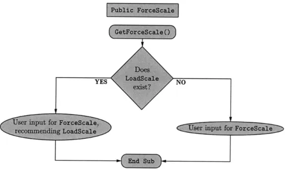
GetForceScale 0 obtains user input for the global variable ForceScale, which sets the scale for the load line and force polygon (e.g. ift = 1001b). If the global variable LoadScale exists, which it typically does because the force polygon follows from load arrows, the script recommends that ForceScale be set to the same value as LoadScale, but will accept any user input. If ForceScale does not exist for some reason, this recommendation is not made, and any input is accepted. GetForceScale is a subroutine, and does not return any value. The source code for this script is found in Appendix A.5. The pseudocode flowchart is found in Figure 3-6.
3.2.5
GetForceSize
GetForceSize () obtains user input for the global variable ForceSize, which sets the height of text notations on the force polygon. If the global variable BowsSize exists, which it typically does because the force polygon is labeled based on Bow's notation, the script recommends that ForceSize be set equal to BowsSize, but will accept any user input. If BowsSize does not exist for some reason, this recommendation is not made, and any input is accepted. GetForceSize is a subroutine, and does not return any value. The source code for this script is found in Appendix A.6. The pseudocode flowchart is found in Figure 3-7.
3.2.6
GetAxialSize
GetAxialSize () obtains user input for the global variable AxialSize, which sets the height of the axial force labels used at the completion of a graphic statics analysis. If the global variable ForceSize exists, which it typically does because the axial forces are derived from the force polygon, which is itself labeled, the script recommends that AxialSize be set to half of ForceSize, but will accept any user input. If ForceSize does not exist for some reason, this recommendation is not made, and any input is accepted. GetAxialSize is a subroutine, and does not return any value. The source code for this script is found in Appendix A.3. The pseudocode flowchart is found in Figure 3-8.
3.2.7
MakePoint
MakePoint (Layer, Location) takes inputs for layer and location and creates a point object with those characteristics. MakePoint is a subroutine, and does not return any
YES
Figure 3-6: Script-Level Subroutine - GetForceScale
YES
any value. The source code for this script is found in Appendix A.12. The pseudocode flowchart is found in Figure 3-9.
3.2.8
MakeLabel
MakeLabel (Layer, Location, Label, Size) takes inputs for layer, location, label text, and label size and creates a text object with those characteristics. MakeLabel is a subroutine, and does not return any value. The source code for this script is found in Appendix A.11. The pseudocode flowchart is found in Figure 3-10.
3.2.9
LabelOverlap
LabelOverlap() takes no inputs, but queries the user to select all labels on the force polygon which represent the same point. LabelOverlap deletes the overlapping labels and replaces them with a single text object containing the selected labels separated by commas. The text height and layer of this hybrid label are based on the height and layer of the first label selected. LabelOverlap is a subroutine, and does not return any value. The source code for this script is found in Appendix A.10. The pseudocode flowchart is found in Figure 3-11.
3.2.10
IntersectLines
IntersectLines (TrimOption) takes a boolean input of Trim0ption, and queries the user for two lines. If those lines, or their extensions, do not intersect, an error message is printed and the user is asked for two new lines. If the lines or their extensions do intersect, a point is generated at the intersection on the same layer as the first line selected. This point is generated by calling another script-level routine, MakePoint. If TrimOption is true and either or both of these lines extend beyond the intersection point, the user is given the option to trim such lines. The option to trim is not offered for any line on which the intersection point does not lie, nor for any curves which are not straight lines (for example, circles used as limiting lines). The trimming of appropriate lines is accomplished by selecting a point on the line beyond the intersection point. IntersectLines is a function, and returns the object ID for the generated intersection point, or returns a null value if no such point was created. The source code for this script is found in Appendix A.9. The pseudocode flowchart is found in Figure 3-12.
3.2.11
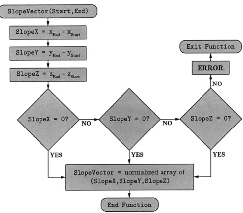
SlopeVector
SlopeVector (Start , End) returns the vector components of the slope of a line which passes between the points Start and End, presuming that said line lies on one of the cardinal planes. This is tested by confirming that at least one of the components of the resulting directional vector is zero. SlopeVector is a function, and returns a nor-malized directional vector of two points which are coplanar on a cardinal coordinate