HAL Id: hal-00659458
https://hal-mines-paristech.archives-ouvertes.fr/hal-00659458
Preprint submitted on 12 Jan 2012HAL is a multi-disciplinary open access archive for the deposit and dissemination of sci-entific research documents, whether they are pub-lished or not. The documents may come from teaching and research institutions in France or abroad, or from public or private research centers.
L’archive ouverte pluridisciplinaire HAL, est destinée au dépôt et à la diffusion de documents scientifiques de niveau recherche, publiés ou non, émanant des établissements d’enseignement et de recherche français ou étrangers, des laboratoires publics ou privés.
Spatial price homogeneity as a mechanism to reduce the
threat of regulatory intervention in locally monopolistic
sectors
Magnus Söderberg, Makoto Tanaka
To cite this version:
Magnus Söderberg, Makoto Tanaka. Spatial price homogeneity as a mechanism to reduce the threat of regulatory intervention in locally monopolistic sectors. 2012. �hal-00659458�
CERNA WORKING PAPER SERIES
Spatial price homogeneity as a mechanism to reduce the threat of
regulatory intervention in locally monopolistic sectors
Magnus Söderberg and Makoto Tanaka
Working Paper 2012-02
Cerna, Centre d’économie industrielle
MINES ParisTech
60, boulevard Saint Michel
75272 Paris Cedex 06 – France
Tél. : 33 (1) 40 51 90 00
January 2012
1
Spatial price homogeneity as a mechanism to reduce the threat of
regulatory intervention in locally monopolistic sectors
Magnus Söderberg a and Makoto Tanaka b
a CERNA, Mines ParisTech, 60 Boulevard St Michel, 75006 Paris, France; E-mail:
magnus.soderberg@mines-paristech.fr, Tel: +33 (0)1 4051 9091; Fax: +33 (0)1 4051 9145.
b National Graduate Institute for Policy Studies (GRIPS), 7-22-1 Roppongi, Minato-ku, Tokyo 106-8677, Japan; E-mail: mtanaka@grips.ac.jp, Phone: +81 (0)3 6439 6000, Fax: +81 (0)3 6439 6010
12 January 2012
Abstract
We claim that a reason for why unregulated investor-owned local monopolies do not always charge the monopoly price is that they are threatened by customer complaints that may lead to retaliations from local elected officials. When investor-owned monopolies are exposed to this threat they will mimic the price(s) of their neighbour(s); the stronger the threat, the higher the spatial price correlation. The threat increases when elected officials have pro-consumer preferences and
neighbours are geographically close. The empirical analysis, based on a complete cross-sectional data set from the Swedish district heating sector in 2007, confirms the theoretical predictions.
Keywords: regulatory threat, district heating, Sweden JEL Classification: L12, L21, L51, L97
2 1. INTRODUCTION
It has been noted that local monopolies owned by private investors do not always charge prices that are significantly higher than those charged by publicly owned monopolies, and/or that the
introduction of formal price regulations does not always reduce prices (Edwards and Waverman, 2006; Stigler and Friedland, 1962; Wallsten, 2001). One may ask, therefore, why local monopolies owned by private investors (IOMs) do not always set their prices at a higher level. Some
commentators have suggested that the explanation may be that local monopolies owned by public bodies (POMs) are not relevant benchmarks since they might not maximise social welfare,1 and others have pointed at the difficulty of designing regulatory models that appropriately incentivise price reductions (e.g. Joskow, 2008). These explanations assume that the price-setting incentives are primarily homogenous within sectors, whereas empirical studies have pointed at substantial price-setting heterogeneity within monopolistic (network) sectors (Altissimo et al., 2006; White, 1996). In the present paper, we propose a new explanation to why IOMs depart from the textbook behaviour, an explanation that is based on heterogeneous threat of regulatory intervention.
Our claim is that locally, unregulated IOMs voluntarily hold back their prices when they are threatened by complaints from customers that are likely to result in retaliations from local elected officials. The probability of a customer complaint is positively correlated with the heterogeneity in pricing behaviour that the customer observes when comparing the price in her/his jurisdiction with the price(s) in neighbouring jurisdiction(s). Vote-maximising elected officials typically have an arsenal of different responses to choose from in this situation, ranging from relatively soft interventions such as more restrictive building/location permit processes and use of fuel types to more extreme
interventions such as receivership (i.e. that the local public administration takes over the responsibility of the utility’s operative work) and expropriation (i.e. that ownership is legally transferred to the local council).2 However, elected officials are either pro-consumer or pro-firm, which affects their
probability to intervene. IOMs respond to this threat by mimicking the prices set by their neighbours, with the level of threat being positively correlated with the spatial price correlation.
Our claim is related to the literature on regulatory threat, which says that firms self-regulate their present profits to gain higher profits in the future (Brunekreeft, 2004; Leidy, 1994; Block and Feinstein, 1986). Firms’ incentive to react to threat has been justified from their desire to reduce the
1 Two established arguments are Niskanen’s (1968) budget-maximising principle and Stigler’s (1971) suggestion about industry capture.
2 Both receivership and expropriation have been used in the locally monopolized electricity distribution sector in Sweden, and re-municipalisation (not renewal of concession contracts) has occurred in the German electricity distribution sector and the French water sector in recent years in response to high consumer prices.
3 overall degree of scrutiny from outside agents, transfer scrutiny to other firms (Decker, 1998) and/or prevent more stringent regulatory activity in the future (Lutz et al., 1998). In previous studies it has been taken as given that a firm’s exposure to threat is positively correlated with its price level, or price cost margin (Glazer and McMillan, 1992; Brunekreeft, 2004; Bawa and Sibley, 1980).3 The validity of this claim hinges on the assumption that an isolated price level is informative to policy makers. However, even if one imposes the weaker assumption that policy makers can react to price changes, this can be an unrealistically strong assumption when outside agents suffer from a lack of cost information.4 As an alternative, it has been suggested that monitoring agents can compare conditions set simultaneously by (many) firms and that this can explain firms’ behaviour relatively well
(Gilpatric et al., 2011).5 In an unregulated market where customers cannot rely on policy makers to effectively monitor monopolies, they can themselves form expectations about the monopolies’ degree of ‘abusiveness’. If customers compare conditions set simultaneously by different monopolies, they can compare their own conditions with those set in neighbouring jurisdictions. The preference for closer neighbours follows from Dixit’s (2003) random matching model, which postulates that individuals are more likely to ‘match’ the closer (according to physical distance or some
socioeconomic criteria) they are located. The presence of strategic interaction between neighbouring jurisdictions has been confirmed empirically in studies on a broad range of local policy setting (e.g. Bordignon et al., 2003; Buettner, 2001; Brueckner, 1998). Customers’ tendency to use conditions in neighbouring jurisdictions as a basis for why they complain about monopolistic conditions was also observed by Söderberg (2008) in his review of a large number of customer complaints in the regulated Swedish electricity distribution sector.
Several studies in the marketing literature suggest that when a price is perceived as unfair, it provokes anger and increases the likelihood of customer responses, e.g. switching of supplier (Antón et al., 2007; Athanassopoulos, 2000; Campbell, 1999).6 Similar arguments have been used to build theoretical models in the economic literature (Di Tella and Durba, 2009; Rotemberg, forthcoming,
3 More recent theoretical studies have extended the earlier models of regulatory threat in different directions, e.g. the pricing decision under the threat of potential divestiture of firms (Tanaka, 2011) and the pricing of a utility with an expanding network facing a threat of regulatory intervention (Chisari and Kessides, 2009).
4 For example, it has been claimed that the lack of relevant (cost) information is the primary complication involved in regulating locally monopolistic utility sectors (Joskow, 2005).
5 Gilpatric et al. (2011) compare two regulatory evaluation mechanisms – one where firms’ present conditions are evaluated based on their previous conditions and one where several firms are compared with each other based on conditions set simultaneously.
6 In the context of local monopoly services, it has been demonstrated that demand is positively related to regulatory compliance (Stafford, 2007).
4 2005). In Rotemberg’s (2005) model, firms internalise that customers react negatively when they become convinced that a price is unfair. Di Tella and Dubra (2009) reach a similar conclusion and show that equilibria exist where customers are not angry.7 Rotemberg (forthcoming) introduces the notion of a reference price that the current price is compared with to form an opinion about whether a price is fair or not. He suggests that this reference price can be a price charged previously by the firm. As pointed out above, the present paper takes an alternative position as it uses prices set
simultaneously by neighbours as reference price(s).
Lastly, we also draw on the literature that focuses on the influence of local political ideology on regulatory decisions. These studies have suggested that left-wing governments tend to be relatively more pro-consumer (Holburn and Spiller, 2002; Holburn and Vanden Bergh, 2006, Besley and Coate, 2003; Cambini and Rondi, 2010). Similar to Biggar and Söderberg (2011), we highlight the influence of local political ideology on the pricing strategies of district heating utilities, even in the absence of any formal regulatory mechanism.
The claim that spatial price heterogeneity is a source of regulatory threat in local monopolistic sectors has not yet been modelled theoretically, and it has only received sporadic empirical attention. The purpose of this paper is to provide a theoretical foundation for this mechanism and to evaluate its existence empirically based on the Swedish district heating sector. This sector consists of a mixture of unregulated IOMs and POMs that are confined by municipal borders. The Swedish district heating sector provides a unique setting for studying monopolies’ price incentives since, contrary to most network sectors, the IOMs are not subject to formal price control mechanisms. Also, the Swedish electoral system can be characterised as bi-partisan where the ruling party/coalition is either left- or right-wing. There is empirical evidence that left-wing local councils in Sweden generally intervene more in markets (Pettersson-Lidbom, 2008), and Biggar and Söderberg (2011) find that the Swedish district heating utilities adopt a more pro-consumer pricing behaviour under left-wing local councils. We utilise a complete cross-sectional data set from 2007 that has not been used before in published work.
Our theoretical model, which can be viewed as a new variant of the Bertrand model, complements existing theoretical explanations for regulatory threat by showing that local monopolists, under certain conditions, have incentives to mimic the prices set by their neighbours. Similar ‘neighbouring’ effects have been observed previously in the context of regulatory threat. For example, Block and Feinstein
7 This is confirmed empirically by Arora and Cason (1996) as they show that firms are more inclined to voluntarily comply with regulatory conditions when they have relatively more customer contacts.
5 (1986) show that the cost of highway construction is reduced after antitrust enforcement in
neighbouring jurisdictions, and Eckert and Eckert (2010) find that firms are more likely to comply with environmental regulations when neighbours have recently been found in violation.
Several empirical studies have looked at firms’ pricing behaviour in response to policy makers’ (likely) actions (Olmstead and Rhode, 1985; Erfle and McMillan, 1990; Driffield and Ioannidis, 2000). The study that is most similar to ours is Ellison and Wolfram’s (2006) investigation of pharmaceutical prices in the U.S. during a period of a relatively intense scrutiny from policy makers. Similar to our study, they suggest that firms voluntarily hold back prices to reduce the threat of regulatory intervention and that firms’ responses are positively correlated with their degree of regulatory vulnerability. However, our study differs from Ellison and Wolfram’s (2006) in terms of both market structure and source of threat since they consider a market subject to competition and when the level of threat is related to the firms’ own price levels.
The paper proceeds with a section that lays the foundation of our theoretical model. Our propositions are presented in Section 3. A background on the Swedish district heating sector is given in Section 4, and the empirical analysis is presented in Section 5. Section 6 concludes.
2. THE MODEL
Consider a set of unregulated locally monopolistic firms i where each firm faces its own demand for heat, qi(pi), and p denotes the price. We assume that i qi′ <0 and limp→∞ qi(pi)=0
i . The cost of
providing the heat is denoted ci(qi(pi)). If the firm is an IOM, its profit is expressed as )) ( ( ) ( ) ( i i i i i i i i p = p q p −c q p
π , where πi(pi) is strictly concave, i.e. πi′′(pi)<0. The monopoly price is denoted m argmax i( i)
i p
p = π , where ′( m)=0.
i i p
π The relevant price range for the firm is
m i i p
p ≤ since raising the price beyond the monopoly price decreases its profit. Note that πi′(pi)>0 holds for m
i i p
p < . Consumer surplus in each district is expressed as =
∫
∞ ′ ′i p i i i i i p q p dp cs ( ) ( ) , where 0 ) ( ) ( =− < ′ i i i i p q p s
c and csi′′(pi)=−qi′(pi)>0for the relevant price range. Thus, csi(pi) is strictly convex. Social surplus in each district is then represented by the sum of the profit and consumer surplus: swi(pi)=πi(pi)+csi(pi). The welfare-maximising price is denoted
) ( max
arg i i
i sw p
p = , where swi′(pi)=0. Maximised social surplus is denoted
i i i i i i i sw p cs p cs w
s ≡ ( )+ ( )≡π + . As the price increases beyond p , the social surplus decreases i
6 assume that swi(pi) is strictly concave, i.e. swi′′(pi)=πi′′(pi)+csi′′(pi)<0. Lastly, we mention some relevant facts that we will come back to later: m
i i i p p p < < , πi(pi)>πi, csi(pi)<csi and i i i p sw
sw( )< hold, since π′i >0, cs′i <0 and sw′i <0, respectively.
2.1 Structure of firms
A fully privately owned firm is only concerned with its own profit. A public firm, on the other hand, is concerned with consumer surplus as well as its own profit. Considering the private and public structures of firms, we define the surplus of firm i as follows:
) ( ) ( ) ( i i i i i i i p p cs p S =π +α , (1) where αi∈
[ )
0,1 .8 When =0 iα , the firm is fully private and only seeks to maximise its profit. When i
α
<
0 , the firm is a public firm that maximises the weighted sum of its profit and consumer surplus. A larger αi implies that the firm has a more public character, putting more emphasis on consumer surplus.9 When
i
α approaches 1, the firm becomes the (local) council itself and seeks to maximise full social surplus. We will discuss this extreme case later.
Noting that csi′′(pi)>0 and αi∈
[ )
0,1 , αicsi′′(pi)<csi′′(pi) holds. After adding πi(pi) on both sides, we obtain ) ( ) ( ) ( i i i i i i i p p cs p S′′ =π′′ +α ′′ ) ( ) ( i i i′′ p +cs′′ p <π , 0 < (2)where the last inequality comes from the strict concavity of swi(pi). Thus, Si(pi) is strictly concave. The maximiser of the firm’s surplus is denoted s argmax i( i)
i S p p = . s i p is unique since ) ( i i p
S is strictly concave. Obviously, the maximiser p for the firm is greater than the full welfare-is
maximising price p for the council, and less than or equal to the full profit-maximising price i m i p for
the fully private firm, i.e. pi < pis ≤ pim. p coincides with is p when im αi is 0.
8 This type of formulation is usually employed in the literature on mixed markets involving private and public firms (e.g. De Fraja and Delbono 1989; Matsumura 1998).
9
i
7 Note that ′( s)=0
i i p
S . It follows from the strict concavity of Si(pi) that Si(pi) is increasing for s i i p p < , i.e. 0 ) ( ) ( ) ( = ′ + ′ > ′ i i i i i i i p p cs p S π α (3)
for pi < pis. Furthermore, Si(pi)>Si holds for pi < pi < pis since Si′(pi)>0 for this price range.
2.2 Expected surplus of firms
Next we introduce a functional relationship between the probability of regulatory intervention and the prices set by the firms. The probability of regulatory intervention is assumed to be a function of the price difference between two neighbouring firms, i.e. θi(pi −p−i). The regulatory authority observes prices as well as introduces price regulation in district i with probability θi(pi −p−i) where θi(⋅) is increasing, i.e. θi′>0. pi −p−i can be both positive and negative. We consider the range of
probability, 0<θi<1, for the relevant price range.10 It should be noted that the probability of intervention is positive even when firm i charges a price below the neighbour’s price. Furthermore, we assume that θi(⋅) is strictly convex, i.e. θi′′>0 for the relevant range.
Once the regulatory authority decides to intervene in district i, price regulation is introduced. We consider that the price will be regulated at p . At this level, the firm obtains a constant surplus, i
i i i i i i i i i i i S p p cs p cs
S ≡ ( )=π ( )+α ( )≡π +α . Considering a risk-neutral firm, we can now express its expected surplus as
i i i i i i i i i i i i p p p p S p p p S ES ( , − )=(1−θ ( − − )) ( )+θ ( − − ) ) ) ( )( ( ) ( i i i i i i i i p p p S p S S − − − = θ − . (4)
The second term on the second line of (4) can be interpreted as a form of expected penalty. When firm
i chooses some price level p given i p−i, its surplus Si(pi) is reduced by Si(pi)−Si with probability θi(pi−p−i). This highlights that the expected surplus of firm i depends not only on its
10 We rule out the extreme cases when the regulatory authority intervenes with 100 percent certainty (θ
i=1), and when there is no risk of intervention (θi=0).
8 own price p , but also on i p−i in the neighbouring district –i. Using the terms of profit and consumer surplus, expected surplus can be written as
)) ( ( i i i i i i i i i i cs cs cs ES=π +α −θ π +α − π +α . (5)
Firm i maximises its expected surplus given the price of neighbouring firm –i. The first-order condition for firm i can be written as
0 ) ( ) 1 ( − ′ − ′ − = = ∂ ∂ i i i i i i i S S S p ES θ θ . (6)
Recall that Si(pi)>Si for pi < pi < pis, Si′>0 for pi < pis, and S′′<0, as discussed in
subsection 2.1. Moreover, note that 0<θi <1, 0θi′> , and θi′′>0, as discussed here. We then have
0 ) ( 2 ) 1 ( 2 2 < − ′′ − ′ ′ − ′′ − = ∂ ∂ ≡ i i i i i i i i i i S S S S p ES θ θ θ φ (7)
for pi < pi < pis regarding the second-order condition.
2.3 The council
Before turning to the analysis of regulatory threat, we explore the decision of the council in relation to the model of the firm. As discussed in the introduction of this section, the council wants to set the price at p to maximise the social surplus i swi(pi) in district i. This coincides with the decision of the firm, which wants to maximise its expected surplus ESi(pi,p−i) when αi approaches 1.
When αi approaches 1, we have ESi =swi −θi(swi −swi)=πi +csi −θi(πi +csi −(πi +csi)) and ESp (1 i)swi i(swi swi) i i = − ′− ′ − ∂ ∂ θ θ . Noting that ′( )=0 i i p w
s and swi ≡swi(pi), we can easily
verify that p satisfies the first-order condition of firm i, i.e. i ∂∂ =0
i i
p ES
, when αi approaches 1. Here we assume that ES with i αi =1 is strictly concave for the relevant range, i.e.
0 ) ( 2 ) 1 ( −θi swi′′− θi′swi′ −θi′′ swi −swi < . (8)
9 3. EFFECTS OF REGULATORY THREAT
We investigate the effects of regulatory threat in detail. As discussed in the previous section, the expected surplus of the firm is affected by the neighbouring price through the probability of regulatory intervention. Thus, even though the firm is a local monopolist, each firm strategically chooses its price in each jurisdiction, taking into account the price(s) of neighbouring jurisdiction(s). This can be regarded as a new variation of the Bertrand model where spatial price competition is driven by regulatory threat.
Technically, we can obtain the Nash equilibrium by solving the first-order conditions (6)
simultaneously. Let us characterise the equilibrium prices (pi*,p−*i) in the following proposition:
Proposition 1. The equilibrium price p is such that *i pi < pi*<pis.
Proof. Noting that ′( s)=0 i i p S , Si(pis)>Si and θi′>0, we have 0 ) ) ( ( * < − ′ − = ∂ ∂ − −= = i s i i i p p p p i i S p S p ES i i s i i θ .
Thus, firm i can make more profit by choosing a price less than pis for any given p*−i. Next, noting that 0<θi <1 and Si′(pi)>0, we have
0 ) ( ) 1 ( * > ′ − = ∂ ∂ − − − = = i i i p p p p i i S p p ES i i i i θ .
This implies that firm i can make more profit by choosing a price greater than pi for any given p*−i. Therefore, p is such that *i pi< pi*< pis. ■
Without any regulatory threat, the firm would have chosen pis. However, once the firm faces some regulatory threat, it strategically charges a price lower than p , even though it is a local monopolist. is
10 In what follows, our analysis is concerned with the relevant price range of pi< pi <pis unless otherwise stated.
We further examine the strategic reaction of the firm under regulatory threat. The first-order condition (6) for firm i yields the best response function pi =BRi(p−i). When the decisions of the firms are ‘strategic complements’, the slope of the best response curve is positive. In contrast, when the decisions of the firms are ‘strategic substitutes’, the slope of the best response curve is negative.11 In the next proposition we show that pi and p−i are strategic complements.
Proposition 2. Prices are strategic complements, i.e. ∂∂2 ∂ >0 −i i i p p ES .
Proof. Noting that Si(pi)>Si, Si′>0, 0θi′> and θi′′>0, we have
0 ) ( 2 > − ′′ + ′ ′ = ∂ ∂ ∂ ≡ −i i i i i i i i i p ESp θ S θ S S ψ . (9) ■
This proposition implies that the slope of the best response curve is positive:
0 ) ( 2 2 2 > − = − = ′ ∂ ∂ ∂ ∂∂ − − i i i i i p ES p p ES i i i i p R B φ ψ . (10)
The current model is different from the standard Bertrand model. Each firm is a local monopolist that faces its own demand. Despite this fact, regulatory threat induces each local monopolist to react strategically, taking into account the price(s) of neighbouring jurisdiction(s). As a result, regulatory threat leads to a positive price correlation among jurisdictions. An interesting question is how the structure of the firm affects its strategic reaction. Thus, we next examine the effects of changing αi on the slope of the best response curve, BRi′(p−i). We obtain the following results:
Proposition 3. When αi increases, the slope of the best response curve decreases, i.e. ∂∂ ′ <0
i i R B α . 11 See e.g. Tirole (1988).
11 Proof. See Appendix 1. ■
If a firm is fully private with αi =0, the slope of the best response curve is the steepest. If a firm gains a more public character with a larger αi, the slope of the best response curve becomes flatter. These results follow from the publicly owned firm’s incentive to restrain its price, taking account of the consumer surplus in its district. Therefore, when αi increases, the slope of the best response curve decreases, and hence the positive correlation of prices among districts becomes weaker.
As discussed in Section 2, when αi approaches 1, the firm becomes the council itself, and the price it chooses approaches p . i p is determined irrespective of the neighbouring price since i p is the i
maximiser of full social surplus swi(pi). Consequently,
i i R B α ∂ ′ ∂
approaches 0 when αi approaches 1.
Lastly, we extend and refine our model by introducing a proxy parameter μi∈(0,1) that represents the strength of regulatory threat. We assume that a higher value of μi corresponds to a situation where the regulatory threat is stronger. Specifically, two situations are worth noting, based on
descriptive statistics presented in Section 4. First, utilities operating under pro-consumer councils will face more severe downward pressure on prices than those operating under pro-firm councils. Thus, it is assumed that μi takes a higher value when elected officials have more consumer-friendly
preferences. Second, neighbours located relatively close to each other are subject to more serious price comparison than distant neighbours. Hence, it is assumed that μi takes a higher value when neighbouring jurisdictions are geographically closer.
Given some observed level of price difference between two districts, the probability of regulatory intervention should be higher when μi is larger. Thus, it is straightforward to rewrite the probability of intervention as μ θi i(pi−p−i).12 The expected surplus of firm i can now be rewritten as
( , ) ( ) ( )( ( ) )
i i i i i i i i i i i i
ES p p− =S p −μ θ p −p− S p −S . (11)
12 We can also assume multiple parameters for the strength of the regulatory threat: for example, a (0,1) i
μ ∈ for the preferences of elected officials and b (0,1)
i
μ ∈ for the geographical proximity of neighbouring districts. Then the probability of intervention can be expressed as a b ( )
i i i pi pi
μ μ θ − − . However, this alteration does not change the main results of the model.
12 In the following, the double bars are used to express all corresponding terms that include μi. We then obtain the following results regarding the effects of changing μi on the slope of the best response curve, BR′i(p−i):
Proposition 4. When μi increases, the slope of the best response curve increases, i.e. i 0
i
BR
μ′ ∂
∂ > .
Proof. See Appendix 1. ■
This proposition implies that the response of a firm to the neighbouring price is positively related to the strength of the regulatory threat. Firms are exposed to stronger regulatory threat when elected officials are more pro-consumer and neighbouring jurisdictions are geographically closer. When μi increases, the slope of the best response curve increases and hence the positive correlation of prices among districts becomes stronger.
4. THE SWEDISH DISTRICT HEATING SECTOR
The district heating technology builds on the principle of centralised heat production where the heat is distributed under high pressure to customers’ properties through a network of underground pipelines carrying hot water or steam. At the customer’s property, a heat exchanger extracts heat energy and the cooler water is returned to the heat centre to be re-heated and re-distributed. District heating meets approximately 50% (or 47 TWh) of the total heat demand in Sweden and it is the most common heating alternative for multi-dwelling houses in 234 of the total 290 municipalities (SCA, 2009; SCB, 2009). Networks only exist in densely populated areas over a certain size and it is rare that networks are connected over municipal borders.
In 2007, 30 % of the utilities were IOM and 36% operated in municipalities with a right-wing dominated council. 13 While ideological composition of the local council must be treated as endogenous in the subsequent analysis, we will argue that IOMs and POMs are structurally similar and can be considered as random samples. This argument is based on the high degree of similarity
13 In our empirical investigation, an investor-owned district heating utility is defined as a utility where private investors control any share > 0 of the utility. Söderberg (2011) shows that private investors tend to determine the economic behaviour of Swedish energy utilities irrespective of whether they are minority or majority owners.
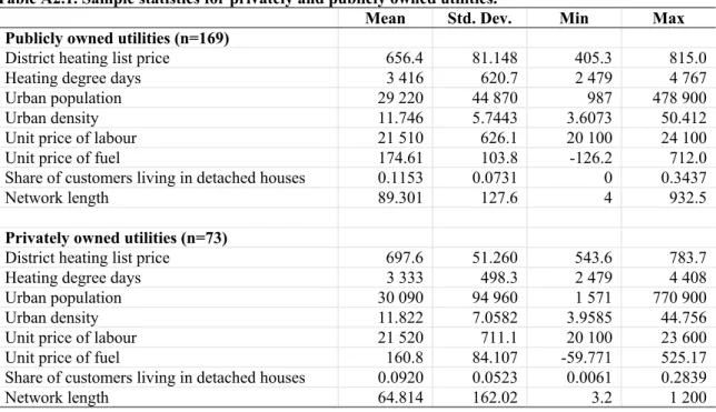
13 between the two sub-samples in terms of climate conditions, population characteristics, input price levels and network characteristics (detailed statistics are provided in Table A2.1 in Appendix 2).
Municipal-level data from 2007 shows that the average price per MWh for a multi-dwelling property that consumes 193 MWh of heat is 653 SEK and 663 SEK when the utility is a POM and operating under left- and right-wing councils, respectively.14 When the utility is IOM, the price is 688 SEK when the council is left-wing and 710 SEK when the council is right-wing. Although these prices are not statistically different, they do indicate that utilities under left-wing councils charge lower prices than those under right-wing councils, and that POMs charge lower prices than IOMs.
Pair-wise correlations between prices in municipality i and its neighbours i− , where i is IOM and
{
1,2,..., −1}
=
−i i is ordered in distance between i and i− , show that the correlation is 0.44 between
i and − i=1 and 0.28 between i and − i=2 (the results are similar when i operates under left- and right-wing councils). The correlations for higher values of i− are insignificant. Similar calculations for when i is POM show that the correlation is 0.31 when − i=1 and the council is left-wing. Correlations for higher values of i− , and when the local council is right-wing, are insignificantly different from 0. The picture that emerges from these descriptive figures is that (i) neighbouring prices are significantly correlated, yet the correlation is generally confined to the closest neighbour, (ii) IOMs are substantially more affected by neighbours’ prices than are their POM counterparts, and (iii) utilities operating under left-wing (rather than right-wing) councils attach more weight to the price of their closest neighbour.
There is no statistics available on complaints about district heating prices, but a recent study on the characteristics of district heating coverage in local and national Swedish newspapers shows that prices are the most frequently covered topic and that the tone is more critical when the utility is an IOM (Palm and Magnusson, 2009). This shows that customers have an effective channel to reach out with their complaints to elected officials. Anecdotal evidence from utility representatives and media reporting also indicates that municipalities can (and do) make decisions that have a substantial impact on utilities’ financial performance.
14 These prices represent the price paid by a multi-dwelling property that is considered to be a ‘national average property’. See Section 5.1 for further details.
14 5. EMPIRICAL EVALUATION
Based on the insights from Section 4, we want to empirically investigate whether p is influenced by i
1 = −i
p , i.e. the price charged by i’s closest neighbour. Propositions 3 and 4 postulate that the relationship between p and i p−i=1 is stronger when i is an IOM and when i faces a stronger regulatory threat. This translates into a functional form that can be written as pi =γWp− 1i= +xiβ, where γ is the parameter denoting the spatial association between p and i p−i=1. W is a weight matrix consisting of predetermined proxies for the level of threat between i and all i− .
To allow public and private utilities to have different values of γ, and for private utilities to respond differently to left- and right-wing dominated local councils, it is necessary to add two additional spatial terms where the elements in the second and third weight matrixes are multiplied with the type of ownership and ownership/political majority, respectively. The measures of ownership and political orientation can be continuous, as in the theoretical model, yet here we use two binary variables where
b takes the value 1 if the utility is classified as an IOM and r takes the value 1 if the local council has
a right-wing majority.15 To increase flexibility, we allow the price variables to be transformed by λ, where λ=
[
−1,1]
and where λ=0 represents the natural logarithm. Hence, the general model that we want to estimate is formulated asi i i i i i p p p pλ =γ1W1 −λ=1+γ2W2 −λ=1+γ3W3 −λ=1+x β+ε , (12)
where the elements in W1, W2, and W3 are calculated as
⎪⎩ ⎪ ⎨ ⎧ − = = −− − otherwise 0 1 for 1 , , , 1 d i w i i i i , ⎪⎩ ⎪ ⎨ ⎧ − = = −− − otherwise 0 1 for 1 , , , 2 bd i w i i i i i and ⎪⎩ ⎪ ⎨ ⎧ − = = −− − otherwise 0 1 for 1 , , , 3 rbd i w i i i i i i . i i
d,− is the Euclidian distance between the centres of the largest urban communities in i and –i. The
inversed distance reduces the weight for more distant neighbours. Similar weighting structures are common in the applied spatial literature (e.g. Lambert et al., 2010; Zhou and Kockelman, 2009; Lee and Yu, 2009).16 However, when only –i=1 is included on the RHS, it is possible that distance is already internalised in the model, and hence the value of including the distance will be investigated more closely.
15
Note that α used in Sections 2 and 3 is related to b as b=1-α.
15 The x vector consists of b, r and cost characteristics. Cost is assumed to be influenced by the unit costs of fuel (p ) and labour (if p ).il 17 In addition, firms that rely on physical networks typically have a cost structure that depends on network characteristics. We include the amount of energy produced (qi) to account for economies of scale in the production, and total network length (A ) to account for i
scale effects in the distribution. Also, two strategic behaviours can influence the pricing behaviour when networks are subject to expansion. First, Chisari and Kessides (2009) point out that a utility can have incentives to keep its price low to attract customers during the initial phase of the expansion, and then raise the price as the network approaches its optimum size. This suggests that price and market share are positively related. However, non-adopters of district heating would prefer a high price to increase public revenue, yet this group will only dominate as long as district heating has a market share below 50% in the heating market. Once the market share exceeds 50%, adopters will be in majority and will lobby for lower prices. This line of argument suggests that the relation between market share and price is negative. To control for these potential effects, we add a variable mi for the
district heating’s market share in the local residential energy market. Utilities’ mix of customer types is accounted for by including share of detached houses, si. Nine firm dummies are also included to
control for instances when a particular utility is responsible for the district heating operation in more than one municipality.
5.1 Data
Data is collected from the Swedish Energy Markets Inspectorate, The Swedish District Heating Association, Statistics Sweden, the ‘Nils Holgersson’s annual price comparisons’, and the
utilities/municipalities directly. The data set is cross-sectional for the year 2007 and represents all 242 municipalities where district heating is a significant source of heating in the largest urban area, excluding Gotland, which is an island. Descriptive statistics and further details about the variables in (12) are provided in Table A2.2 in Appendix 2.
The price p is the average price (fixed plus variable) paid per MWh for a multi-dwelling property i
that consumes 193 MWh of heat and requires 3 860 m3 of water pass-through per year. The
correlations with prices for other standardised customer types (80MWh, 500 MWh and 1 000 MWh) are high (between 0.94 and 0.96), which means that p can be viewed as the average price for all i
multi-dwelling properties.
16 Fuel price is total costs of fuels divided by total amount of kWh produced. This price can be negative since utilities are paid to dispose of public waste, which sometimes is a substantial fuel type. Labour price is average municipal salary (net local taxes) in the public sector. This is preferred to figures based on utilities’ own accounting statements since it eliminates the risk of including rents captured by strong unions and self-rewards by executives.
5.2 Estimation
The derivation of an estimable spatial autoregressive model is not covered here since it has been thoroughly dealt with elsewhere (e.g. Mobley, 2003; Revelli, 2006; Zhou and Kockelman, 2009). Estimating (12) with the non-linear least square estimator, i.e. assuming strict exogeneity, shows that the specification suffers from over-parameterisation. A grid search approach starting with λ=−1 and increasing in steps of 0.1 until λ=1 is therefore applied, showing that the residual sum of squared (RSS) for λ=1 is not significantly higher than the RSS for any other value of λ. This confirms previous findings that linear price models perform well in comparison with unconstrained transformations when firm heterogeneity is unobserved (Cropper et al., 1988).
As we proceed, two problems can be noted. First, the three terms containing p−i are endogenous by construction (LeSage and Pace, 2009) and, second, the residuals εi are likely to be heteroscedastic.18
Instrumental variable approaches with heteroscedasticity-consistent standard errors are offered by both 2SLS and two-stage, or ‘optimal’, GMM (OGMM),19 yet Lin and Lee (2010) note that OGMM is more efficient and potentially more robust. Kelejian and Prucha (1998) argue that a subset of
neighbours’ covariates can be used as instruments to arrive at consistent spatial parameters. We chose this strategy and use neighbours’ fuel and labour prices as instruments for p-i. Further endogeneity
problems can occur if qi is correlated with εi. Such correlation can occur from unobserved property
characteristics. We use share of energy delivered to industrial customers (indi) and population in
urban areas (popi) to control for this potential endogeneity. Although utilities determine the size of the
network themselves, A is treated as exogenous since decisions to extend the network are typically i made several years prior to the actual construction. In Section 4 we showed that public and private utilities are similar when comparing fundamental supply and demand conditions. bi is therefore
treated as exogenous. Ideological composition of the local council can be endogenous to local
18 For example, heteroscedasticity can occur from unobserved variation in network age since some recently established utilities might want to use revenues to finance network expansions. Utilities operating mature networks can therefore be expected to have lower price variability.
19 Kelejian and Prucha (2010) report that the maximum likelihood estimator is significantly biased in the presence of heteroscedasticity.
17 government tariffs.20 The indicator variable for right-wing majority (ri) is instrumented with ri,t-2,
which refers to the situation in the previous electoral period.
An OLS estimation is displayed in Column (a) in Table 1. Column (b) shows the output for when p-i, qi and ri are treated as endogenous, using the OGMM estimator. The results are consistent in terms of
signs and significance levels, but γ2 (γ3) increases (decreases) in magnitude as the exogeneity
assumptions are relaxed. Column (c) shows (12) when di,−i is excluded from the weight matrices. Comparing the RSS values for Column (b) and (c) shows that including di,−i reduces RSS by over 6 %. One can also observe that (c) is not as well-behaved as (a) and (b), which shows that it is important to incorporate the distance between neighbours in order to arrive at reasonable estimates. This finding supports Proposition 4.
Based on estimates in Column (b), the average predicted price charged by POMs (669.2 SEK/MWh) is lower than the price set by IOM under left-wing councils (670.4 SEK/MWh), which in turn is lower than the price set by IOMs under right-wing councils (713.4 SEK/MWh). Although these prices are not statistically different, they point in the same direction as Proposition 1. As expected, there is no evidence that POMs take the prices of their closest neighbours into consideration. IOMs operating under left-wing councils (
γ
1+γ
2), i.e. when the councils are relatively pro-consumer, internalise 50% of the price adjustments made by their closest neighbours. The positive sign ofγ
1+γ
2 lends support to Proposition 2 and the fact thatγ
1<γ
1+γ
2 is consistent with Proposition 3. We have already established thatd
i−,−i1=1 has a substantial role in identifying the relation betweenp
i and1 = −i
p
and that this supports Proposition 4. Further support for Proposition 4 is provided by the fact thatγ
1+
γ
2>
γ
1+
γ
2+
γ
3, i.e. that pro-consumer preferences of elected officials increase the threat. The combination of private ownership and the pro-firm preferences of right-wing councils (γ
1+
γ
2+
γ
3) is apparently strong enough to statistically eliminate the threat of intervention.
20 A strategically behaving council can increase the price when income goes up, and Leigh (2005) shows that income (among several other socio-economics factors) influences voting behaviour.
18
Table 1. Estimation output.
OLS
(a) OGMM
a
(b) OGMM (c)
Variable Mean SE Mean SE Mean SE
1 1 1 , − = − = −i i i p d 0.0245 0.0239 0.0161 0.0235 1 1 1 , −= − = −i i i id p b 0.3275 ** 0.1450 0.4843** 0.2059 1 1 1 , −= − = −i i i i ibd p r -0.0227 0.2672 -0.6252 0.4779 1 = −i p 0.2707 0.2502 1 = −i ip b 0.6741 0.5182 1 = −i i ibp r -0.9566 * 0.4921 bi 12.011 16.161 1.1954 21.248 -453.87 354.52 i ib r 14.697 19.346 50.794 34.914 687.66 ** 341.47 qi 0.0464 ** 0.0194 0.0576*** 0.0203 0.0647 *** 0.0218 i A -0.2552 ** 0.0886 -0.2763*** 0.0876 -0.2863 *** 0.0901 f i p 0.1065 ** 0.0528 0.0994** 0.0479 0.1073 * 0.0556 l i p 0.0114 * 0.0067 0.0121* 0.0063 0.0053 0.0080 mi -49.450 30.854 -34.654 30.775 -31.138 29.391 si -207.85 *** 70.907 -219.44*** 68.247 -185.68 ** 79.268 Constant 437.38 *** 142.44 421.10*** 133.01 382.11 *** 166.92 Ownership
dummies Yes Yes Yes
Hansen’s J 8.245 5.522
Hansen’s P>J 0.221 0.238
R2 0.453 0.446 0.375
No. obs. 242 242 242
Notes: * p < 0.10, ** p < 0.05, *** p < 0.01. SE are robust to arbitrary heteroscedasticity. a Instruments: f i i i p d−,−1=1 −=1, bidi−,−1i=1p−fi=1, ri,t−2bidi−,−1i=1p−fi=1, di−,−1i=1p−li=1, bidi−,−1i=1pl−i=1, l i i i i t i bd p r,−2 −,−1=1 −=1, indi, popi, ri,t−2bi.
Other coefficients reveal that p increases for higher qi i and decreases for higher A which is i
consistent with the view held by industry representatives and the results by Biggar and Söderberg (2011). Input prices are positively correlated with pi. The tests of Hansen’s J show that instruments
are correctly excluded from the main equation and uncorrelated with εi in both Columns (b) and (c).
6. CONCLUSIONS
In this paper we claim that a plausible explanation for why unregulated investor-owned local monopolies do not always charge the monopoly price is that doing so may lead to customer
19 prices with those in neighbouring jurisdictions, and the probability of a complaint is positively
correlated with the degree of spatial price heterogeneity. Elected officials have incentives to intervene when customers (i.e. voters) complain, yet the probability of intervention is reduced when elected officials have pro-firm preferences. We show that when utilities are subject to regulatory threat that originates from spatial price comparisons, the equilibrium price is located between the efficient and monopoly prices. Also, prices charged by neighbouring utilities are strategic complements, meaning that their prices are positively correlated. The spatial price correlation between neighbours increases when IOMs are exposed to relatively strong threat, i.e. when elected officials have pro-consumer preferences and neighbours are geographically close.
The empirical analysis is based on a complete cross-sectional data set from the Swedish district heating sector in 2007. This sector is unique in that it consists of local monopolies that are owned by both private investors (IOM) and municipalities (POM), yet the monopolies are not subject to any formal price regulation. The analysis supports the theoretical predictions by showing that 1) POMs tend to set lower prices than IOMs; 2) IOMs that operate under left-wing councils (i.e. councils that are relatively pro-consumer) have lower prices than IOMs under right-wing councils; 3) IOMs under left-wing councils internalise as much as 50% of their neighbours’ prices; and 4) when the threat of intervention is lower, i.e. when IOMs operate under right-wing councils, there is no sign that they take their neighbours’ prices into consideration.
Policy-wise one can conclude that the threat of regulatory intervention can effectively reduce IOMs’ incentive to use their marker power, yet a favourable situation for consumers is fragile since a change in the council’s ideological preferences can reduce the threat, which may lead to a substantial price increase.
REFERENCES
Altissimo, F., Ehrmann, M., Smets, F., (2006), Inflation persistence and price-setting behaviour in the Euro area. A summary of the IPN evidence, European Central Bank, Occasional Paper Series, No. 46. Antón, C., Camarero, C. and Carrero, M., (2007), The mediating effect of satisfaction on consumers’ switching intention, Psychology & Marketing, Vol. 24(6), pp. 511-538.
Arora, S. and Cason, T.N., (1996), Why do firms volunteer to exceed environmental regulations? Understanding particulation in EPA’s 33/50 program, Land Economics, 72(4), pp. 413-432. Athanassopoulos, A.D., (2000), Customer satisfaction cues to support market segmentation and explain switching behaviour, Journal of Business Research, 47, pp. 191-207.
20 Bawa V.S. and Sibley D.S., (1980), Dynamic behaviour of a firm subject to stochastic regulatory review, International Economic Review, Vol. 21, No. 3, pp. 627-642.
Besley, T. and Coate, S., 2003. Elected versus appointed regulators: theory and evidence. Journal of the European Economic Association 1, 1176-1206.
Biggar D. and Söderberg, M., (2011), The effect of future price expectations on customers’ willingness to make sunk investments in reliance on a monopoly service, CERNA Working Paper 2011-06.
Block M.K. and Feinstein J.S., (1986), The spillover effect of antitrust enforcement, Review of Economics and Statistics, Vol. 68, pp. 122.131.
Bordignon, M., Cerniglia, F. and Revelli, F., (2003), In search of yardstick competition: a spatial analysis of Italian municipality property tax setting, Journal of Urban Economics, 54, pp. 199-217. Brueckner, J.K., (1998), Testing for strategic interaction among local governments: the case of growth controls, Journal of Urban Economics, 44, pp. 438-467.
Brunekreeft, G., (2004), Regulatory threat in vertically related markets: the case of German electricity, European Journal of Law and Economics 17: 285-305.
Buettner, T., (2001), Local business taxation and competition for capital: the choice of the tax rate, Regional Science & Urban Economics, 31, pp. 215-245.
Cambini, C. and Rondi, L., 2010. Regulatory independence and political interference: evidence from EU mixed-ownership utilities’ investment and debt. Fondazione Eni Enrico Mattei Working Paper No. 458.
Campbell, M.C., (1999), Perceptions of price unfairness: antecents and consequences, Journal of Marketing Research, Vol. 36, pp. 164-175.
Chisari, O. and Kessides, I., (2009), Pricing dynamics of network utilities in developing countries, Review of Network Economics, Vol. 8, No. 3, pp. 212-232.
Cropper, M.L., Deck, L.B. & McConnell, K.E. (1988). On the choice of functional form for hedonic price functions. Review of Economics and Statistics, 70, 668-675.
Decker, C.S., (1998), Implications of regulatory responsiveness to corporate environmental
compliance strategies, Working paper, Dep. of Business Economics and Public Policy, Kelley School of Business, Indiana University.
De Fraja, G. and Delbono, F. (1989), Alternative Strategies of a Public Enterprise in Oligopoly, Oxford Economic Papers, 41, 302–311.
Di Tella, R., and Dubra, J., (2009), Anger and regulation, MPRA Paper No. 14442.
Dixit, A., (2003), Trade expansion and contract enforcement, Journal of Political Economy, 111(6), pp. 1293-1317.
Driffield, N. and Ioannidis, C., (2000), Effectiveness and Effects of Attempts to Regulate the UK Petrol Industry, Energy Economics 22: 369-381.
21 Eckert, H. and Eckert, A., (2010), The geographical distribution of environmental inspections, Journal of Regulatory Economics, Vol. 37, No. 1, pp. 1-22.
Edwards, G. and Waverman, L., (2006), The effects of public ownership and regulatory independence on regulatory outcomes, Journal of Regulatory Economics, 29(1), pp. 23-67.
Ellison, S. F. and Wolfram, C., (2006), Coordinating on Lower Prices: Pharmaceutical Pricing Under Political Pressure, RAND Journal of Economics 37(2): 324-340.
Erfle, S. and McMillan, H., (1990), Media, Political Pressure, and the Firm: The Case of Petroleum Pricing in the Late 1970s, Quarterly Journal of Economics 105(1): 115-134.
Gilpatric, S.M., Vossler, C.A., McKee, M., (2011), Regulatory enforcement with competitive endogenous audit mechanisms, RAND Journal of Economics, 42(2), pp. 292-312.
Glazer, A. and McMillan, H., (1992), Pricing by the Firm Under Regulatory Threat, Quarterly Journal of Economics 107(3): 1089-1099.
Holburn, G. L. F. and Spiller, P. T., 2002. Interest group representation in administrative institutions: The impact of consumer advocates and elected commissioners on regulatory policy in the United States. POWER working paper 002, University of California at Berkeley.
Holburn, G. L. F. and Vanden Bergh, R. G., 2006. Consumer capture of regulatory institutions: The creation of public utility consumer advocates in the United States. Public Choice 126, 45-73. Joskow, P., (2008), Incentive regulation and its applications to electricity networks, Review of Network Economics, 7(4), 547-560.
Joskow, P., (2005), Regulation and Deregulation after 25 Years: Lessons Learned for Research in Industrial Organization, Review of Industrial Organization, vol. 26(2), pages 169-193.
Kelejian H.H. and Prucha I.R., (1998), A generalized spatial two-stage least squares procedure for estimating a spatial autoregressive model with autoregressive disturbances. Journal of Real Estate Finance and Economics, Vol. 17, pp. 99-121.
Kelejian H.H. and Prucha I.R., (2010), Specification and estimation of spatial autoregressive models with autoregressive and heteroscedastic disturbances, Journal of Econometrics, Vol. 157, No. 1, pp. 53-67.
Lambert D.M., Brown J.P. and Florax R., (2010), A two-step estimator for a spatial lag model of counts: theory, small sample performance and an application, Regional Science and Urban Economics, Vol. 40, No. 4, pp. 241-252.
Lee L.-F. and Yu J., (2010), Some recent developments in spatial panel data models, Regional Science and Urban Economics, Vol. 40, No. 5, pp. 255-271.
Leidy, M.P., (1994), Rent dissipation through self-regulation: the social cost of monopoly under threat of reform, Public Choice, 80, pp. 105-128.
Leigh, A., 2005. Economic voting and electoral behaviour: how do individuals, local, and national factors affect the partisan choice? Economics and Politics 17, 265-296.
LeSage J.P. and Pace R.K., (2009), Introduction to spatial econometrics. CRC Press/Taylor & Francis Group: London.
22 Lin X. and Lee L.-F., (2010), GMM estimation of spatial autoregressive models with unknown heteroscedasticity, Journal of Econometrics, Vol. 157, No. 1, 34-52.
Lutz, S. Lyon T, and Maxwell J., (1998), Strategic quality choice with minimum quality standards, Discussion paper no 1793, London: Centre for Economic Policy Research.
Matsumura T. (1998), Partial Privatization in Mixed Duopoly, Journal of Public Economics, 70, 473– 483.
Mobley L. R., (2003), Estimating hospital market pricing: an equilibrium approach using spatial econometrics, Regional Science & Urban Economics, Vol. 33, pp. 489-516.
Niskanen, W.A., (1968), Nonmarket decision making: the peculiar economics of bureaucracy, The American Economic Review, 58(2), pp. 293–305.
Olmstead, A. L. and P. Rhode, (1985), Rationing without Government: The West Coast Gas Famine of 1920, American Economic Review 75(5): 1044-1055.
Palm J. and Magnusson D., (2009), Medias rapportering om fjärrvärme, Report 2009:32, Fjärrsyn. (In Swedish).
Pettersson-Lidbom, P., 2008. Do parties matter for economic outcomes? A regression-discontinuity approach. Journal of the European Economic Association 6, 1037-1056.
Revelli F., (2006), Performance rating and yardstick competition in social service provision, Journal of Public Economics, Vol. 90, pp. 459-475.
Rotemberg, J.J., (forthcoming), Fair pricing, Journal of the European Economic Association. Rotemberg, J.J., (2005), Customer anger at price increases, changes in the frequency of price adjustment and monetary policy, Journal of Monetary Economics, 52, pp. 829-852.
Stafford, S.L., (2007), Can consumers enforce environmental regulations? The role of the market in hazardous waste compliance, Journal of Regulatory Economics, 31(1), pp. 83-107.
Stigler , G.J. and Friedland, C., (1962), What can regulators regulate? The case of electricity, The Journal of Law and Economics, 47, pp. 84-99.
Stigler, G.J., (1971), The theory of economic regulation, Bell Journal of Economics & Management Science, 2, pp. 3–21.
Söderberg M., (2011), The role of model specification in finding the influence of ownership and regulatory regime on utility cost: the case of Swedish electricity distribution, Contemporary Economic
Policy, 29(2), pp. 178-190.
Söderberg M., (2008), Uncertainty and regulatory outcome in the Swedish electricity distribution sector, European Journal of Law and Economics, Vol. 25, No. 1, pp. 79-94.
Tanaka, M., (2011), The Effects of Uncertain Divestiture as Regulatory Threat, Journal of Industry, Competition and Trade, 11(4): 385-397.
23 Wallsten, S.J., (2001), An econometric analysis of the telecom competition, privatization, and
regulation in Africa and Latin America, The Journal of Industrial Economics, 49(1), pp. 1-19. White, M.W., (1996), Power struggles: explaining deregulatory reforms in electricity markets, Brookings Papers on Economic Activity. Microeconomics, 1996, pp. 201-250.
Zhou B. And Kockelman K.N., (2009), Predicting the distribution of households and employment: a seemingly unrelated regression model with two spatial processes, Journal of Transport Geography, Vol. 17, No. 5, pp. 369-376.
24 APPENDIX 1
Proof of Proposition 3
Note that πi′>0, 0πi′′< , 0csi′< and csi′′>0, as stated in the beginning of Section 2. It follows from 0
< ′ i
w
s and swi′′<0 in the beginning of Section 2 that 0<πi′<−c ′si, and 0<csi′′<−πi′′. Thus, we obtain i i i i′cs′′<π′′cs′ π . (13)
Note that πi >πi, and csi <csi′, as stated in the beginning of Section 2. It follows from i i i i i i cs cs sw sw =π + <π + = , that ) ( 0<πi −πi <− csi −csi . (14)
Next, rearranging (8) in subsection 2.3 yields
i i i i i i i i i′sw′− ′′sw −sw < ′sw′− − sw′′ − < ( ) (1 ) 0 θ θ θ θ (15)
The first inequality comes from swi′<0, swi <swi, 0θi′> , and θi′′>0. Thus, i
i i
i′sw′ − − sw′′
< (1 )
0 θ θ holds. Noting this and 0<θi<1, we have i i i i i i i i cs θ cs θπ θ π θ ′′− ′ ′ < ′ ′ − − ′′ − <(1 ) (1 ) 0 (16)
Then, it follows from (14) and (16) that:
) ) 1 ( )( ( ) ) 1 )(( (πi −πi −θi csi′′−θi′cs′i <− csi −csi θi′πi′− −θi πi′′ . (17)
We now check the sign of ⎟
⎠ ⎞ ⎜ ⎝ ⎛− + = ∂∂ ∂∂ ∂ ′ ∂ i i i i i i i i i R B αφ α ψ φ α 12 φ ψ . The sign of ii R B α ∂ ′
∂ depends on the sign
inside the bracket. Noting that (13) and (17) hold, we obtain:
) )( 1 ( i i i i i i i i i i i i = ′ − ′cs′′− ′′cs′ ∂ ∂ + ∂ ∂ − θ θ π π α φ ψ φ α ψ