Discriminating Noise from Chaos in Heart Rate Variability: Application to Prognosis in Heart Failure
by
Natalia M. Arzeno
S.B. Electrical Science and Engineering Massachusetts Institute of Technology, 2006
Submitted to the Department of Electrical Engineering and Computer Science in Partial Fulfillment of the Requirements for the Degree of
Master of Engineering in Electrical Engineering and Computer Science at the Massachusetts Institute of Technology
May 2007
Copyright 2007 Natalia M. ArzenoV. All rights reserved.
The author hereby grants to M.I.T. permission to reproduce and
to distribute publicly paper and electronic copies of this thesis document in whole and in part in any medium now known or hereafter created.
Author
Department of Electrica Engineering and Computer Science May 25, 2007 Certified by Chi-Sang Poon arch Scientist i Supervisor Accepted by thur C. Smith
1
Engineering Chairman, Department Committee on Graduate ThesesMASSACHUSETTS INS E OF TECHNoLOGy
OCT
0
3
2007
BARKER
VDiscriminating Noise from Chaos in Heart Rate Variability:
Application to Prognosis in Heart Failure
by
Natalia M. Arzeno
Department
Submitted to the
of Electrical Engineering and Computer Science
May
25,
2007
In Partial Fulfillment of the Requirements for the Degree of
Master of Engineering in Electrical Engineering and Computer Science
ABSTRACT
This thesis examines two challenging problems in chaos analysis: distinguishing deterministic
chaos and stochastic (noise-induced) chaos, and applying chaotic heart rate variability (HRV)
analysis to the prognosis of mortality in congestive heart failure (CHF).
Distinguishing noise from chaos poses a major challenge in nonlinear dynamics theory
since the addition of dynamic noise can make a non-chaotic nonlinear system exhibit stochastic
chaos, a concept which is not well-defined and is the center of heated debate in chaos theory. A
novel method for detecting dynamic noise in chaotic series is proposed in Part I of this thesis.
In Part II, we show that linear and nonlinear analyses of HRV yield independent
predictors of mortality. Specifically, sudden death is best predicted by frequency analysis
whereas nonlinear and chaos indices are more selective for progressive pump failure death.
These findings suggest a novel noninvasive probe for the clinical management of CHF patients.
Thesis Supervisor: Chi-Sang Poon
Title: Principal Research Scientist
Table of Contents
Introduction
...
11
PartI
...
15
Volterra Series Approach for Distinguishing Deterministic and Stochastic
Noise in Chaotic Series...
15
Chapter 1 Chaos Theory and Occurrence ...
17
1.1
W hat is ch aos? ...
... ... . .17
1.2
R outes to chaos ...
. 18
1.3
N oise and chaos ...
. 19
1.4
C haos in biological system s...
20
1.5 C h ao s M ap s...
2 0
Chapter 2 Nonlinearity and Chaos Detection Theory...
27
2.1 Volterra Autoregressive Series Theory...
27
2.2 D etection of C haos Level...
28
Chapter 3 Numerical Simulation Results for Characterization of the Chaotic Maps.... 31
3.1 Effect of integrator, integration step, and discretization on the Lorenz map... 31
3.2 Choice of Parameters for Chaotic Maps ... 33
3.3 Effect of Dynamic and Measurement Noise on the Logistic and Henon Maps... 36
Chapter 4 Noise Discrimination Algorithms ... 41
4.1 Volterra Autoregressive Series for Detection of Dynamic Noise... 41 4.2 Successive Substitution Volterra Autoregressive Series for Detection of Measurement
4.3 Effect Successive Substitution Volterra Autoregressive Series Parameters and Noise
D iscrim ination A lgorithm ...
43
Chapter 5 Results and Discussion of Noise Discrimination Algorithms...
49
5.1 Results of Noise Identification Algorithm on Chaotic Maps...
49
5.2
Algorithm Applications and Limitations ...
53
5.3 Future Algorithms for Noise Discrimination in the Presence of Chaos ...
54
Part II
...
57
Risk Stratification of Mortality in Mild to Moderate Heart Failure by Heart
Rate Variability Analysis...
57
Chapter 6 Congestive Heart Failure and Heart Rate Variability ...
59
6.1 C ongestive H eart Failure ...
59
6.2 H eart R ate V ariability ...
60
6.3 Previous Studies for Characterization of CHF and Mortality Prediction ...
62
Chapter 7 Data and Experimental Methods...67
7.1 Congestive H eart Failure D ata...
67
7.2
Heart Rate Variability Analysis Indices ...
69
7.3 Statistical M ethods...
. . 74
Chapter 8 Training Set and Test Set Results ...
79
8.1 R esults for Training Set ...
79
8.2 A nalysis of T est Set ...
. 85
Chapter 9 Complete Data Set Results...
89
9.1 ROC Analysis of Complete Data Set...
89
9.3 Cox Proportional Hazards Model for Sudden Death and Progressive Pump Failure... 91
Chapter 10 Discussion of Results and Significance of Study...95
10.1 Analysis and Interpretation of Results...
95
10.2 Study Limitations and Future Work ...
101
List of Figures
Figure 1.1. Bifurcation diagram for the logistic map...
21
Figure 1.2. Chaotic attractor of the Henon map for a
1.4 and b
=
0.3...
22
Figure 1.3. Chaotic attractor of the Ikeda map for B 0.82... 23
Figure 1.4. Mackey-Glass chaotic thousand-point series with a = 0.2, b = 0.1, n = 10.5... 25
Figure 2.1. N um erical titration algorithm ... 29
Figure 3.1. The results of different integration of the Lorenz map are classified by order of integrator (rows) and integration step (columns). The squares represent points that are not chaotic (N L should be zero)... 32
Figure 3.2. Noise limit graphs for chaos maps. The red circles indicate the particular parameters that w ere analyzed... . 35
Figure 3.3. Effect of increasing measurement noise on the detected intensity of chaos for different regions of the logistic m ap ... 37
Figure 3.4. Effect of increasing dynamic noise on the detected intensity of chaos for different regions of the logistic m ap... 38
Figure 3.5. Effect of increasing measurement noise on the detected intensity of chaos for different regions of the Henon map with b=0.3... 39
Figure 3.6. Effect of increasing dynamic noise on the detected intensity of chaos for different regions of the Henon m ap with b=0.3... 40
Figure 4.1. Logistic map with dynamic noise (thin, black line) and SSVAR estimation (thick, blue line) after 31 iterations ... 44
Figure 4.2. Cost functions of SSVAR. The signal is a logistic map with dynamic noise (variance = 0.003). The numbers to the left and right of each cost function represent the index of the first eight iterations... 45
Figure 4.3. Cost functions of SSVAR for measurement noise. The signal is a logistic map with measurement noise (variance = 0.03). The thick blue curve is the cost function of the first iteration ... . . 4 6 Figure 4.4. Close-up of SSVAR cost functions for measurement noise. The signal is a logistic map with measurement noise of variance 0.03. The iteration numbers of SSVAR are w ritten in the m iddle of the curves. ... 46
Figure 5.1. Accuracy of noise identification for chaos maps with dynamic and measurement n o ise ... 5 2 Figure 8.1. Average noise limit and LF/HF for survivor and non-survivor group. The error bars show the standard error for each segment. The values for each 12-minute segment were averaged over 3-hours to yield smooth curves... 79
Figure 8.2. Results of ROC analysis. The bar graphs plot the area under the ROC curves. The
shaded bars represent higher values for the survivors while solid bars represent
lower values for the survivors. The ranking of the AUC for each parameter is written
on top of each bar...
. . 8 1
Figure 8.3. ROC curves for accurate and random-like mortality detectors...
83
Figure 8.4. Kaplan Meier Curves for linear and chaos HRV indices. The most significant (NL
and LF/HF) HRV indices are plotted in the left graph. The right graph illustrates the
Kaplan Meier curve for the classic SDNN, the newer nonlinearity detection rate
index, and the not-significant high frequency. The blue HF curves are for the cutoff
value of 478 Ms
2where 25 of 50 subjects were above the cutoff value... 85
Figure 8.5. Support vector machine classification errors for test set (n = 358) from training setboundaries. Only the HRV index combinations that yielded a lower error than the
best ROC detection (error = 125) are plotted... 86 Figure 8.6. Support vector machine classification of mortality using NL (24 h) and LF/HF (24 h).
The training set is plotted in the left panel and the test set is superimposed on the training set in the right panel for better observation of classification errors. The survivors are represented by the red marks and the nonsurvivors by the blue marks. The white lines indicate the support vectors... 87
Figure 9.1.
Figure 9.2.
Kaplan Meier curves for entire data set. The left frame-short-term correlation
exponent, LF/HF (day), and SDNN-plots the best mortality predictors. The right
frame plots two worse, but significant, predictors (24 hour NL and SampEn) and a
nonsignificant predictor (night H F). ...
91
Kaplan-Meier curves for sudden death and progressive pump failure. The left panel
plots the survival curves for the day NL, short-range correlation exponent, and night
TP in sudden death. The right panel plots the survival curves for SDNN, short-range
correlation exponent, and day LF/HF in progressive pump failure. The cut-off values
were determined by the median HRV indices in the entire population... 93
List of Tables
Table 5.1. Measurement and dynamic noise variances tested for the chaotic maps... 50
Table 5.2. SSVAR results for dynamic noise. ...
50
Table
5.3.
SSVAR results for measurement noise...
51
Table 5.4. Noise identification accuracy for chaos maps. ...
53
Table 7.1. Patient group characteristics ...
68
Table 8.1. Indices with highest accuracy in ROC analysis...
80
Table 8.2. Proportional Hazards Results for Significant Univariate and Multivariate Predictors.84
Table 8.3. R O C results for test set ...
85
Table 8.4. Best 2-D support vector machine classifiers...
87
Table 8.5. Best3-D support vector machine classifiers...
88
Table 9.1. Indices with highest accuracy in ROC analysis for complete data set ...
89
Table 9.2. Results for Cox proportional hazards analysis of the complete data set ...
90
Table 9.3. Significant univariate predictors of sudden death...
92
Introduction
Chaos analysis has presented countless challenges from the full understanding of the seemingly random, yet deterministic, systems to detection of chaotic dynamics in experimental data, to the application of chaotic system properties in the real world. Many have proposed solutions to these challenges, but the full potential of chaotic system analysis is yet to be discovered. Two remaining challenges in chaos analysis are discussed in this thesis: identifying noise as stochastic or deterministic in chaotic series, and determining the risk of death of patients with congestive heart failure (CHF) from the chaotic heart rate series.
The detection of chaos in noisy signals has been approached in various manners [1-3]. Similarly, the effect of noise on chaotic signals and noise-induced chaos have been previously explored [4-6]. However, only one group has approached the identification of the type of noise in chaotic signals [7], an interesting problem since noise identification can lead into further understanding of the underlying system dynamics. Strumik et. al. [7] found dynamic noise in the H6non and Ikeda maps could be represented as measurement "pseudonoise" of the Cauchy distribution and designed an algorithm based on correlation entropy for noise identification which, though reliable for dynamic noise, was not reliable for measurement noise. The algorithm in [7] is also limited by the lack of systems for testing, thus a new noise identification algorithm is essential. The first part of the thesis introduces an algorithm which identifies if well-known chaotic maps are contaminated with additive dynamic noise -resulting from noise that affects the future chaotic dynamics at each time point- or deterministic measurement noise-where the noise is superimposed on the chaotic dynamics- mimicking the effect of a measuring device. Chapter
1
focuses on chaos theory: the definition of chaos, the ways chaos can be achieved and the effect of noise on chaotic systems. In addition, various physiological systems that exhibit chaotic dynamics are explained in the chapter. The second part of Chapter1
defines the chaos maps used for the analysis-logistic, Henon, Ikeda, Lorenz, and Mackey-Glass-as well as their previous applications or realizations in nature. The nonlinear modeling and chaos detection theory are described in Chapter 2. Chapter 3 delves into the choice of parameters for the chaos maps and the effect of dynamic and measurement noise on the logistic and H6non maps. The approach to system noise identification by means of Volterra series approximations and the parameters used in the simulations are described in Chapter 4. Chapter 5 statesthe results and limitations of the study, where improvements and alternate algorithms are suggested in the last section of the chapter.
Congestive heart failure, the inability of the heart to pump enough blood to the body, is the common end of various diseases such as coronary artery disease and congenital heart disease. Two kinds of death commonly accompany CHF: sudden cardiac death and death from progressive pump failure. Pump failure death often occurs after progressive worsening of the CHF symptoms whereas sudden death implies a fatal electrical event (arrhythmic event) taking place during a time of clinical stability and is typically a manifestation of reduced left ventricular function [8, 9]. Heart rate variability (HRV) analysis in the congestive heart failure population has become of interest over the past decade as a predictor for specific kinds of death in CHF. Linear and nonlinear analysis of HRV provides a non-invasive, inexpensive method to detect autonomic changes and aid the physician's treatment of the condition. Results of previous studies rely heavily on the advancement of the disease in the subject group as well as the number of subjects included in the study such that studies often present contradictory results [10]. In addition, previous studies typically focus on a subset of HRV indices, analyzing traditional time- and frequency-domain parameters in combination with either complexity or nonlinear indices. The lack of a comprehensive set of HRV indices in a single study prevents the identification of independent predictors of mortality. The second part of the thesis focuses on combining several traditional linear and less-applied nonlinear-including chaotic-indices of heart rate variability to determine the significant univariate and multivariate predictive factors of all-cause death, sudden death, and progressive pump failure death in patients with congestive heart failure. Chapter 6 characterizes congestive heart failure and heart rate variability. The physiological markers of CHF are discussed along with the different modes of death that accompany the disease. The use and significance of heart rate variability in a variety of situations is discussed, including previous works using HRV for risk stratification of mortality in CHF. The dataset is described in Chapter 7 along with the definition and calculation of the HRV indices used in the analysis. The results for the three types of survival analysis-receiver operating curve (ROC), support vector machine classification (SVC), and Cox proportional hazards-are stated in Chapters 8 and 9. Chapter 8 encompasses the ROC and SVC results from division of the data into a training set and a test set. The Cox hazards results for the training set are also stated for characterization and validation of the training set. The results for analysis of the complete data set are described in Chapter 9 for all-cause mortality, sudden
death, and death from progressive heart failure. Chapter 10 encompasses the analysis of the results, main contributions of the study, and future work.
Part I
Volterra Series Approach for Distinguishing
Chapter 1 Chaos Theory and Occurrence
Over the past decades, an interest in studying, defining, and characterizing chaotic series has emerged. The challenges of defining what specific properties are comprised in a chaotic series, how to define equations such that they mimic chaotic occurrences in nature, and how to detect the presence and level of chaos in a signal have been approached in different ways. In this chapter, the various sections explain the particular characteristics of chaotic series, the different ways chaos can be reached, the effect of noise on chaotic series, and several physiological systems which exhibit chaotic dynamics. Section 1 delves into the definition of chaos, the specific properties of the apparently random but deterministic dynamics in the time-domain and the phase-space, and introduces a relative measure of chaos intensity in noise-free systems. The equations that define chaotic dynamics only do so for certain parameters, where a slight change in the equation parameters can result in a periodic series. The most common routes to chaos through the variation of a specific parameter in the equation, as well as the topological properties that are implied by the routes to chaos, are described in Section 2. Chaotic dynamics in nature are often contaminated by noise. Section 3 presents various works on the effect of noise on chaotic series and introduces the controversy of "noise-induced chaos." Section 4 explores different occurrences of chaos in physiological systems, both in anatomical structures and reactions to particular stimuli. The chaos maps used in analyzing the noise identification algorithms are defined in Section 5.
1.1 What is chaos?
Chaotic series are often mistaken as randoirness, when in reality they are deterministic nonlinear dynamical systems with great dependence on initial conditions. For example, two chaotic series described by the same equations but with slightly different initial conditions (e.g. difference of 10-6) will have diverging trajectories. A series is classified as chaotic if it fulfills three conditions [11]:
1. it displays sensitivity to initial conditions 2. it is topologically transitive
3. its periodic orbits are dense
The sensitivity to initial conditions of a signal is quantified by the Lyapunov exponent. The Lyapunov exponent determines the presence and degree of chaos in noise-free systems and corresponds to the
average separation rate of neighboring trajectories. In a one-dimensional map the Lyapunov exponent is defined as [11]:
A = lim -fog
_r
" iM rn og df (fxo) (1.1)-- o n
|xI|
n-+ i dxThe Lyapunov exponent has been shown to be independent of initial conditions (xo) and is positive for series with sensitivity to initial conditions.
Topological transitivity and topological mixing express the evolution of the series trajectories; although chaotic dynamics are deterministic, they are asymptotically unpredictable. The condition of dense periodic orbits requires any interval to contain infinite periodic orbits with high period. If the chaotic series is expansive-iterations of points in any given subinterval will eventually cover the entire interval after a sufficient number of iterations-then all three conditions for chaos are satisfied.
Chaotic dynamic in a system usually only cover a subset of the phase space, such that the chaotic behavior falls on an attractor. The attractor is defined by three properties: it is a closed invariant set, it attracts an open set of initial conditions, and it is minimal [12]. The stability of the trajectories depends on the convergence to the attractor (Poisson) and the convergence within the attractor (Lyapunov) [13]. If the attractor exhibits sensitivity to initial conditions, it is called a strange attractor [12]. Strange chaotic attractors are characterized by their complex geometrical structure, at least one positive Lyapunov exponent, and fractal (non-unity) dimension.
1.2 Routes to chaos
In dynamical systems, there are three major routes to chaos [13]: 1. period-doubling
2. intermittency
3. quasiperiodicity destruction
The period-doubling route to chaos is reached by a series of period-doubling bifurcations, , up to a critical parameter where there are infinite periods. Past the critical parameter, the system becomes unstable, according to Lyapunov, with aperiodic oscillations and exhibits chaotic properties. Maps which reach
chaos through the period-doubling route, such as the H6non map, are characterized by a dimension between 2 and 3 and a strange attractor with a horseshoe shape [13]. The intermittency route to chaos is characterized by a sudden transition from regular oscillations to chaos. The phenomenon of intermittency occurs when chaotic dynamics are interspersed with periodic-like behavior soon after the critical parameter. In the course of intermittency, the structure of the phase space and the basin of attraction can be radically changed with a single bifurcation, resulting in a crisis. The final route to chaos, destruction of a quasiperiodic orbit occurs when a torus is destroyed in phase space such that the new trajectories have a fractal dimension [13]. The three routes to chaos have been previously shown in low- and high-dimensional systems, where all three routes can exist for the same dynamical system as characterized by exploring different regions and directions in the parameter space.
1.3 Noise and chaos
The effects of dynamic noise in chaotic series, both in additive and multiplicative form, have been previously studied in theory and applications. In the present study, the focus will be on dynamic noise of the additive form. Though several studies have agreed on the existence of noise-induced chaos, others [14] with stricter mathematical definitions argue noise affects the nonlinear properties of the series but its stochastic nature prevents the result from being defined as chaotic. Gassmann [6] studied the effect of stochastic noise in the time series to find a state of interest in a chaotic signal. He defined three regions of interest depending on the variance of the added noise, where the region with largest noise caused dramatic shortening of transients. Gao [4, 5] later focused on dynamic noise converting a highly periodic system to a system with chaos-like motions, where the chaos can arise from changing between two periodic states or between a periodic state and a metastable chaotic state. Like Gaussmann, Gao found three regions of different behavior such that certain noise intensities resulted in Brownian-like motion and others in chaotic-like motions. In addition to inducing chaos in a signal, additive dynamic noise can also stabilize stochastic oscillations, excite oscillations, and induce on-off intermittency and phase transitions, such that in a first-order transition a small change in the control parameter drastically changes the output [15].
The effects of additive measurement noise have not been well studied in chaotic signals since it does not contribute to the chaotic dynamics. The addition of noise to the clean signal, resulting in the observed series, prevents a periodic series from being kicked into the chaotic attractor. In addition, the
superposition of noise onto a chaotic series would only shadow the underlying dynamics rather than force the signal into a different regime.
1.4 Chaos in biological systems
Chaos characterizes numerous biological and physiological systems both in health and disease state. Anatomical structures, such as the His-Purkinje system, chordae tendineae, the vascular tree, and the lung tree contain fractal properties [16]. Many studies over the past decades have concentrated on cardiac [16-20] and neural [17, 20-22] chaos, analyzing the change in chaotic dynamics for a variety of stimuli and subjects with different pathologies, as well as controlling harmful chaotic dynamics such as those arising in cardiac arrhythmias. Additionally, the metabolic system is comprises a large-scale biochemical system which, when simplified to a few variables, also exhibits chaotic dynamics [17, 23]. For example, the metabolic pathway converts the free energy in glucose into adenosine triphosphate (ATP), which is then converted to adenosine diphosphate (ADP). For certain amplitudes and frequencies of sugar influx, the fluctuations in the concentration of ADP are chaotic [17]. Changes in the chaotic attractor's dimension may also indicate a pathology such as in epilepsy, where a "petit mal" seizure has been found to dramatically change the neural chaotic attractor and decrease its dimension [20, 21]. The analysis of chaotic dynamics present in chemical interactions, anatomical structure, and physiological systems allows for better physical understanding and modeling of systems for the characterization and control of diseases.
1.5 Chaos Maps
Various equations have been developed for the purpose of studying chaotic dynamics more in depth or mimicking those that occur in nature. In this chapter, traditional chaotic maps are defined. Sections 1 and 2 introduce the logistic and H6non maps respectively, low-order discrete maps in 1 and 2 dimensions which have been widely used in chaos studies. Section 3 presents a more complex discrete map, the Ikeda map, which contains sinusoidal terms and describes instances of chaos in optics. Two continuous maps, the Lorenz map and the Mackey-Glass equation, are described in Sections 4 and 5. The multi-dimensional Lorenz differential equations are the basis of chaos theory and have led to the creation of various chaotic maps such as the H6non map. The Mackey-Glass equation is used to represent chaotic series of high complexity, where the high order results from the delay in the differential equation.
1.4.1
Logistic Map
The logistic map, a simple non-linear system, depicts the population growth equation in discrete-time as:
xn+I = rxn (1 - xn),1 (1.2)
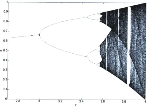
where x, characterizes the dimensionless population at time n. The equation is typically applied with 0 r 4 such that x always maps to the interval [0,1]. At r=3 the logistic map is 2 and period-doubling continues until r-3.569946 [12]. The chaotic regime begins at x ~ 3.57, but is interrupted by periodic windows, the intermittency route to chaos. This phenomenon can be observed in the bifurcation diagram in Figure 1.1.
Ii
3.2 3.4 3.6 3.8
Figure 1.1. Bifurcation diagram for the logistic map.
1.4.2
Henon Map
The Henon map was developed as a manner of studying strange attractors, such as those described by Lorenz, in a two-dimensional discrete manner. The equations for this map are:
(1.3) =n+= bxn 0.9 0.8 0.7 0.6 x 0.5 0.4 0.3 0.2 0.1 01 2.8 3 4 __4
where a is controlled to keep the system trajectories from escaping to infinity and b dictates the folding and contraction of the attractor [12]. Typically, b is kept constant at 0.3 while a is varied to characterize the system (a=1.4 is often used to describe a chaotic system). Contrary to the logistic map, the Henon map is invertible, such that each point corresponds to a unique trajectory. The Henon map is also dissipative and contains trajectories which diverge to infinity unlike the Lorenz map where all trajectories converge towards the attractor [24].
0.1 0. 0.2 0.1 0 -0. -0. -0. -0. 2. 3 -1.5 -1 -0.5 0 0.5 1 1.5 x
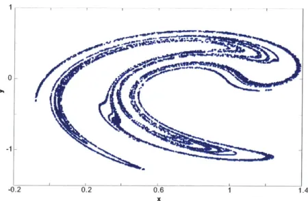
Figure 1.2. Chaotic attractor of the Hnon map for a = 1.4 and b = 0.3.
1.4.3 Ikeda Map
The Ikeda map demonstrates chaotic attractors in optics. Ikeda modified the traditional method of observing optical bistability, an example of first order phase transition in a system far from thermal equilibrium, and showed that the instabilities of light transmitted by a ring cavity systems exhibit chaotic behavior for certain parameters [25]. The Ikeda map is a two-dimensional map described by a complex
number z = x + iy:
f(z)=p+Bexp i- a JZ.
+|_zr
(1.4)
The algorithm can also be written in two real dimensions [26]: xwts = p + B(xn COS t - y, sin ta
y1+1 = B(xn sin tn + yn COS t" ) where the system is chaotic for certain values of B and tn is described as:
a
t 1+x+y (1.6)
The values used were p = 1, K = 0.4, and a = 6, while B was the variable parameter. The chaotic attractor of the Ikeda map is illustrated in Figure 1.3.
--0.2 0.2 0.6 1 1.4
x
Figure 1.3. Chaotic attractor of the Ikeda map for B= 0.82.
1.4.4 Lorenz Map The Lorenz equations are:
x =-Ox +oy
j=-xz+rx-y,
(1.7)z
=xy -bzwhere a (Prandtl number), r (Rayleigh number), and b greater than zero and the dot represents differentiation with respect to a dimensionless time.
In Lorenz's original study, he applied the model with the parameters a = 10 and b = 8/3, in agreement with Saltzman's model [27]. These values were used by Lorenz, along with a time step of 0.01, for numerical integration in order to characterize the system's convective properties. Lorenz found certain parameters could yield solutions that oscillate irregularly, settling on a strange attractor with fractal dimension between 2 and 3. These oscillations occur for r values past the critical bifurcation:
= (cT-+ b +3)
rH = ,) (1.8)
such that Lorenz published his results for the supercritical value r=28-rH ~ 24.74 for the specific parameters used. There exist intermittent windows of periodicity for28 < r < 313. The three largest windows occur for r in the approximate intervals (99.524, 100.795), (145, 166), and (214.4, 313) [12].
The Lorenz equations resemble those from previous studies by Rayleigh and Saltzman which modeled flow in a layer of fluid of uniform depth with a constant temperature difference between the two surfaces. Each variable is proportional to a property of the system: x to the intensity of the convection motion, y to the temperature difference between currents, and z to the deviation from the linear temperature profile. A mechanical model of the Lorenz equations was developed in the 1970s [12]. The model consists of a waterwheel with leaking cups. Water is poured steadily into the cup at the top of the waterwheel and depending on the flow rate of the water the waterwheel can remain stationary, rotate steadily, or, for high flow rates, rotate erratically. Additional changes can be made to the model by modifying the brake on the wheel or changing the tilt of the table on which the waterwheel rests.
1.4.5 Mackey-Glass Equation
The Mackey-Glass equation describes physiological systems and characterizes acute diseases such as white-cell production dynamics and the irregular breathing pattern of Cheyne-Stokes respiration [28, 29]. The Mackey-Glass single-variable equation is [28]:
d= ax(t - r) bx(t), (1.9)
dt 1+x"(t -r)
where t is the time interval, - is the delay dependence, and a, b, and n are parameters that can be altered to achieve periodicity or chaos. The complexity of the system relies heavily on the delay of the differential equation, which is proportional to the dimension of the chaotic attractor. The multistable property of the system causes a heavy reliance on the initial conditions, where periodicity or chaos can result from the same system with different initial conditions [30]. Similar to the Lorenz map, the integration step and sampling of the continuous-like signal affect the titration results. In this study, the Mackey-Glass signals were calculated as in a previous study with an integration step of 0.1 seconds, and sampling every 4 seconds [3]. A chaotic Mackey-Glass series is plotted in Figure 1.4.
1.4
0.6
0.2
1
2
3
4
time (seconds) x 105
Chapter 2 Nonlinearity and Chaos Detection Theory
The Volterra autoregressive series (VAR), a powerful tool for detecting nonlinearity comprises the basis of the algorithms for distinguishing dynamic and measurement noise in chaotic series. A summary of the theoretical basis of VAR, a modification on the traditional Volterra series proposed by Barahona and Poon, is presented in Section 1. The effect of noise on chaotic series cannot be studied without ensuring the contaminated signal is in fact chaotic. Section 2 describes the numerical titration technique [3], where the algorithm output provides sufficient proof of the existence of chaos in short, noisy series.
2.1 Volterra Autoregressive Series Theory
The Volterra autoregressive series (VAR) detects nonlinearity in short data series contaminated with additive and dynamic noise [31]. This method orthogonalizes the traditional Volterra series through a Gram-Schmidt procedure by applying the Wiener series expansion. The Volterra kernels can thus be estimated by recursively applying cross-correlation techniques, while introducing the limitation of a white noise Gaussian input of infinite length. The restriction on the input is eliminated by applying Korenberg's algorithm [32] which estimates the Volterra series for arbitrary signals. The VAR method moreover feeds the output as the delayed input into the Volterra series, allowing the current data point (x) be predicted by a polynomial expansion of previous points with degree d and memory KC:
ao±a' ,j+a2X2± 2 +d
xn -- ao+ ai
]xn-I
+ a2 xn-2 +e
+ aK xn-K+ aK+i x I + aK+2 Xn-J Xn-2 + *** ± aM-J Xn-K(2.1)
M-1
- 1 am zm(n)
m=0
where setting d
1
models a linear time series. The model can be modified to include additive dynamic (,n) and measurement (e,,) noise:Xn =ao-1-a I n-I+ a25 n-2+**0 +ajc5n-A+acx -I +alc+2xn-Jxn-2+ e+ aM-1 n-1+ 'n
M-1
- a, 'mrm(n)+5n (2.2)
m=0
and Yn = 3n+en
where ,, is the orbit of the attractor including dynamic noise, and y,, is the observation after the inclusion of additive noise.
The goodness of fit of the models is quantified by the normalized sum-of-square errors:
N N
c(c, d ) 2 = (x-nKC, d) - yn )2
Y(n-
)2 .(2.3)n=1 n=
The optimal model is defined as that which minimizes the Akaike information criterion:
C(r) = log e(r) +r / N . (2.4)
Two models are proposed to discriminate between stochastic chaos induced by dynamic noise and deterministic chaos in the presence of measurement noise respectively. Though the VAR algorithm cannot distinguish between dynamic and measurement noise, its equations seem to model dynamic noise better than measurement noise. One of the models implements the successive substitution VAR (SSVAR) algorithm, a modification on the VAR algorithm which is more responsive to measurement noise. The SSVAR algorithm iteratively applies the VAR algorithm to the synthesized data, subtracting an error term each time, until the VAR coefficients and the synthesized data converge. This ensures dynamic noise is not modeled in the synthesized data. Thus, for data contaminated with dynamic noise, as long as the error subtraction does not modify the underlying system dynamics, VAR should produce a lower error, and consequently a lower C(r), than SSVAR. For measurement noise, SSVAR should yield the lower C(r).
2.2 Detection of Chaos Level
Numerical titration [3] quantifies the intensity of chaos in a signal, in a manner similar to a chemical titration where the signal acts as the acid and noise acts as the base. This method presents several
advantages over traditional methods. Nonlinear measures such as detrended fluctuation analysis require long sets of data and complexity estimates such as entropy measures do not characterize the nonlinear properties of the signal. In addition, a positive Lyapunov exponent, the traditional measure for chaos detection and quantification, can only be accurately applied to ideal noise-free systems whereas numerical titration has proven an effective measure of chaos for noisy, short data sets.
Noise limit (NL), the output of numerical titration, is a relative measure of the chaos intensity in the series, where a positive NL is sufficient to confirm the existence of chaos. The input to numerical titration is a time series, such as heart rate variability for disease screening. Nonlinear detection is performed on the input with the Volterra autoregressive series, where the input is considered nonlinear if the approximated nonlinear model yields a better fit than the linear model. The best fitting signal is determined by the Akaike information criterion and significance is established with an F-test. If the signal is determined to be linear, it is non-chaotic and NL=O. For a nonlinear signal, a small amount of noise
-1% of the variance- is added to the signal and the nonlinear detection is performed again. The noise addition and nonlinear detection are recursively performed until the signal is not determined to be nonlinear. The positive NL thus characterizes the amount of noise necessary to mask the signal's chaotic dynamics. The numerical titration process is illustrated in Figure 2.1.
Noise Limit Linear
Volterra % added noise
HRV -- y Nonlinear __
Detection
Nonlinear Add % white noise
Figure 2.1. Numerical titration algorithm
The numerical titration technique has been proven successful in yielding NL>O for signals with a positive Lyapunov exponent in standard routes to chaos for several maps including the logistic map, Curry-Yorke discrete map, Mackey-Glass equations, and Lorenz map. In addition, numerical titration has successfully
identified chaos in high order systems such as a Mackey-Glass map with dimension twenty [3]. However, it should be noted that titration cannot provide insight into the dynamics of a system with a negative Lyapunov exponent, where nonlinearity is not detected.
Chapter 3 Numerical Simulation Results for Characterization
of the Chaotic Maps
This chapter explains the parameter selection procedure for the discrimination algorithm, the sampling of the Lorenz map for the creation of a chaotic series, and the chaotic maps. Section 1 examines the effect of the integrator and sampling step for continuous maps, specifically the Lorenz map, on the detected chaos level. The maps for testing the noise discrimination algorithms were chosen such as to represent various non-chaotic and chaotic regions as well as all of the main routes to chaos. The choice of parameters for the discrete and continuous maps is explained in Section 2. Finally, Section 3 investigates the effect of dynamic and measurement noise on periodic and chaotic regions of the logistic and H6non maps.
3.1 Effect of integrator, integration step, and discretization on the Lorenz
map
The nonlinearity detection step in numerical titration requires a discrete signal with uniform spacing in time. For continuous maps this implies a downsampling step, where the discrete signal to be titrated contains uniformly-spaced samples of the continuous-like integrated signal. Thus the integrator, integration step, and discretization affect the resulting map and its level of chaos. The choice of integrators is limited by the necessity of a fixed-time solver. The choice of integrator-Euler's method (first order), Heun's method (second order), or fifth order Runge-Kutta-affects the proximity of the discrete-time integration to a continuous-time integration. The higher order incorporates more terms into the integration and thus provides the most accurate computations. The choice of integration step is essential due to similar reasons: a smaller integration step will yield a better approximation of the discrete signal to a continuous signal, yet a decrease in the integration step causes a significant increase in computation time. The discretization, the sampling of the signal after integration, has a different effect on the system since undersampling prevents an accurate description of system dynamics and oversampling may cause numerical titration to falsely identify the system as non-chaotic since the Volterra series would be calculated based on linearized segments.
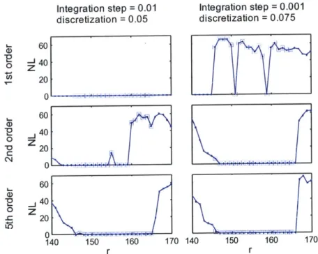
Figure 3.1 illustrates the importance of the integrator order and integration step in the Lorenz map. Letellier found that though any sampling of less than 0.040 seconds will fulfill the Nyquist criterion, the upper value of the discretization step for a first-order integrator (0.0265 seconds) is less than the ideal value for a second-order integrator (0.064 seconds), such that higher-order integrators can be applied with larger discretization steps while preserving the chaotic dynamics of the Lorenz map [33]. The first-order integrator, the Euler method, does not recognize the chaotic signals for the larger integration step and identifies non-chaotic regions as chaotic for the smaller integration step. The importance of the integration step is seen most clearly for the second-order integrator, where the smaller integration step classifies all the regions except for one (r = 146) as chaotic or non-chaotic. The high accuracy achieved with the fifth-order integrator diminishes the role of the integration step such that both integration steps only misclassify one non-chaotic signal as chaotic with a miniscule noise limit (NL<2).
Integration step = 0.01 Integration step = 0.001
discretization = 0.05 discretization = 0.075 60 0 J40 20 0 i 4 i i-I 1 i-O 60 40 Z 20 C 40 (D. 0 . lliF r-20 0 140 150 160 170 140 150 160 170 r r
Figure 3.1. The results of different integration of the Lorenz map are classified by order of integrator (rows) and integration step (columns). The squares represent points that are not chaotic (NL should be zero).
3.2 Choice of Parameters for Chaotic Maps
The parameters for the different maps were chosen such as to describe various non-chaotic and chaotic regions. The variable parameter for the logistic map, r in
x 171 =-" rx (J - xI), (3.1)
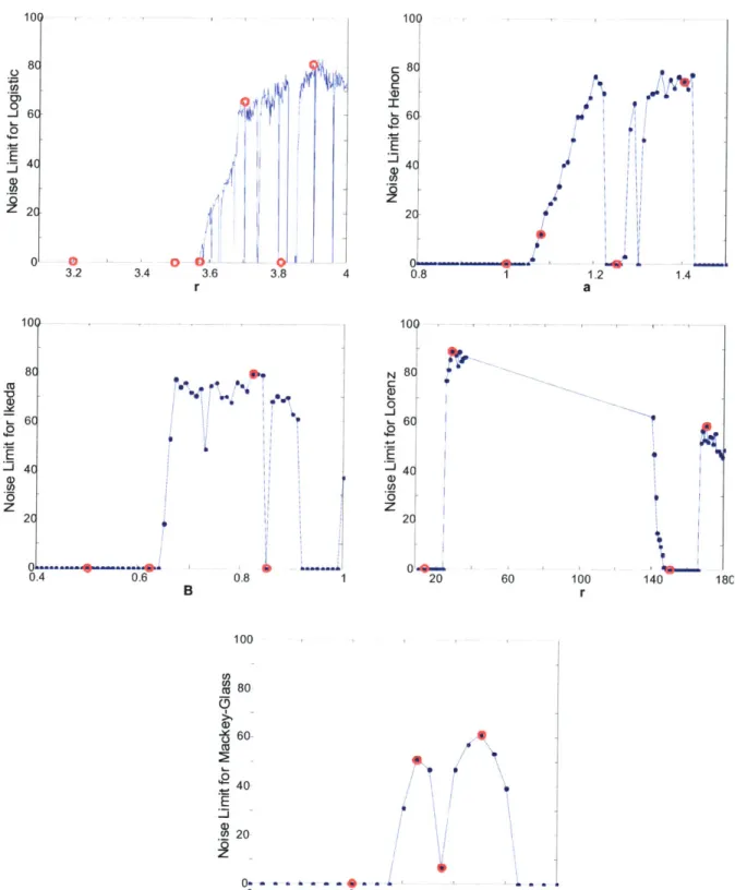
was chosen to convey four different regions of the bifurcation diagram. The chosen parameter values and the map region for the well-studied logistic map were: r-3.2 (period-2), r-3.5 (period-4), r-3.568759 (period-16), r-3.7 (low chaos), r-3.8282 (intermittency), r--3.9 (high chaos) [12]. The parameters for the other maps were chosen by examination of the chaos level at different values. Graphs of the noise limit for different parameter values of each map are plotted in Figure 3.2 where the red circles indicate the parameters used in the study.
The variable parameter in the H6non map, a in
xi=y, +1 - ax~
(3.2) y1i+ bx,,
was chosen as to represent a periodic region (a=1), a low chaos region (a=1.08), a non-chaotic region surrounded by chaos (a= 1.25), and a highly chaotic region (a= 1.4).
The variable parameter for the Ikeda map, B in
x,+, = p + B(x cos tl - y,, sin t,, ) y,1+ = B(x,, sin tf, + y, cos t,1 )
was chosen as to represent a series long before chaos is reached (B=0.5), a periodic series close to the start of chaotic dynamics (B=0.62), a highly chaotic series (B=1.25), and a non-chaotic series surrounded by chaos (B=1.4).
The variable parameters for the continuous series, the Lorenz map and the Mackey-Glass equation were similarly chosen to encompass non-chaotic regions away from chaos, various chaos levels, and low or no chaos regions where a slight parameter change in either direction would largely increase the chaos level. In the Lorenz map
S=-ox + OY
=-xz+rx -y, (3.4)
z
= xy - bzr was chosen as 14, 28, 150 and 170. The Mackey-Glass equation
dx _ax(t-r) _bx(t)
(3.5)
dt -+x"(t-r)
was analyzed for n=8, 9, 9.75, and 10.5. The fewer points in the Mackey-Glass map in Figure 3.2 results from the extensive computations required to create the series.
10J
.1h
3.6 3.8 4 0 C 6C E 4C 2CC
0.8 81 10' 8( 6C 4C 2C 0.4 0.6 PI ----B 0.8 100 100 N C 0 J 0Z
M
80 60-0 LIO 40 E 20 6 8Figure 3.2. Noise limit graphs for chaos maps. The red circles
8 6 4C 2C 0 20 60 100 r 140 18C 10 12
indicate the particular parameters that were analyzed.
8( -i6( 0 -E4C 2C 30 . 3.2 3.4 0
Le
1.2 a '~ I, I I 1.4 Ca .0 Ezi
100 O 13.3 Effect of Dynamic and Measurement Noise on the Logistic and Henon
Maps
A positive noise limit can be a result of an intrinsically chaotic system or a system driven into chaos by noise. Similarly, a non-chaotic system can be such because of the linearity of the signal or randomness induced by measurement noise. Though the noise-free system can never be perfectly extracted from a noisy signal, the identification of the driving noise in the system-measurement or dynamic-can provide insight into system properties. The following sections describe the effects of measurement and dynamic noise on the logistic map and the H6non map, examining different routes to chaos and signals with
diverse chaos intensities.
3.3.1 Definition of Dynamic and Measurement Noise
Dynamic noise was defined as noise added in every time step such that it affected the calculation of future data points. For multidimensional maps such as the Henon map, noise was only added in one of the dimensions:
x =y +1-ax2 ±4
n + n n n+ I
Yn + I , (3.6)
= X
where 6 is the dynamic noise component and i is the observation. Measurement noise was added to a complete noise-free map, such that the noise was superimposed on the signal to form the observation and did not affect the signal dynamics. The logistic map contaminated with measurement noise can be represented as:
x = r,(1 -x,),(3.7)
x~x+e
where . is the measurement noise component and X is the observed series. The applied noise was random Gaussian noise generated in Matlab.
3.3.2 Effect of Noise on the Logistic Map
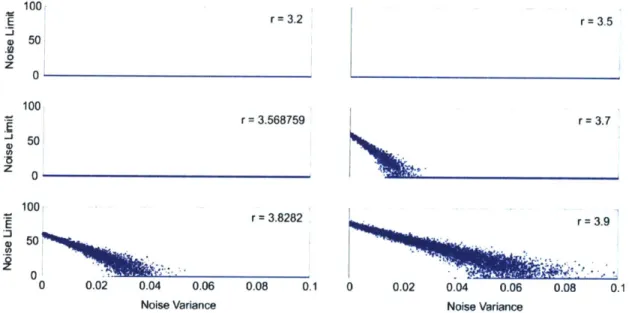
The intensity of chaos in a signal is dependent both on the chaotic background, the intensity of the noise, and the type of noise contaminating the system. The following figures illustrate this dependence with the logistic map. When measurement noise is added to a non-chaotic signal such as the logistic map in the period-doubling regions (Figure 3.3) the map dynamics are not changed, and the added randomness of the noise is not mistaken as nonlinearity such that the noise limit remains at zero. However, measurement noise plays an important role in the chaos intensity of the maps in the chaotic regimes. As can be seen in Figure 3.3, as the noise variance increases, the chaos level, measured by the noise limit, decreases. The noise limit will be zero when the randomness of the noise overshadows the chaotic dynamics of the signal. Thus, the intensity of the underlying chaotic dynamics is proportional to the noise variance required to drive the chaos level to zero. This relation is illustrated in Figure 3.3, where the seemingly linear trend of decreasing noise limit with increasing noise variance intercepts the x-axis at the highest noise variance for the most chaotic map (r=3.9).
100 10r =3.2 r =3.5 E 0 50 0 Z 0 100 r =3.568759 r =3.7 -j 501 0 0 100 r=3.8282 r 3.9 50 0 0.02 0.04 0.06 0.08 0.1 0 0.02 0.04 0.06 0.08 0.1
Noise Variance Noise Variance
Figure 3.3. Effect of increasing measurement noise on the detected intensity of chaos for different regions of the logistic map.
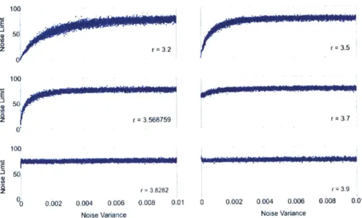
Contrary to measurement noise, which affects the noise limit of already chaotic maps, the addition of dynamic noise has the largest effect on non-chaotic maps. Figure 3.4 shows slight or no increase in the noise limit of maps that are intrinsically chaotic after the addition of dynamic noise. However, noise-free
non-chaotic maps become increasingly chaotic with the inclusion of dynamic noise, saturating at a maximum noise limit value for high noise variances. This effect can be seen in Figure 3.4, where the noise limit increases more rapidly with increasing noise for maps which are closer to chaotic regions, where the noise limit for the period- 16 logistic map (r-=3.568759) saturates for lower noise variances than the noise limit for the period-2 logistic map (r=3.2).
100 50 0 100 50 r 3,568759 0' 100 50 r = 3.7 r = 3.8282 r = 3.9 0 0.002 0.004 0006 0.008 0.01 0 0.002 0.004 0.006 0.008 0.01
Noise Variance Noise Variance
Figure 3.4. Effect of increasing dynamic noise on the detected intensity of chaos for different regions of the logistic map.
3.3.3 Effect of Noise on the Hknon Map
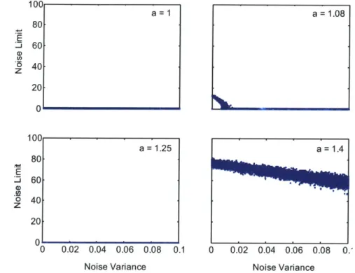
The effect of measurement noise on the detected chaos level of the Hdnon map is similar to that of the logistic map. Periodic regimes retain a noise limit of zero while chaotic maps experience a decrease in the noise limit with an increase in the measurement noise variance. However, as can be seen in Figure 3.5 the chaotic region with the highest noise limit (a=1.4) never becomes non-chaotic in the experimental noise variance range. This suggests a chaotic system more robust to measurement noise than the logistic map with similar noise-free noise limits.
100 a=1 a =1.08 80 E - 60 *5 40 z 20 0 100 a =1.25a1. 80 o 40 z 20 01 0 0.02 0.04 0.06 0.08 0.1 0 0.02 0.04 0.06 0.08 0.'
Noise Variance Noise Variance
Figure 3.5. Effect of increasing measurement noise on the detected intensity of chaos for different regions of the Henon map with b=0.3.
As with the logistic map, the addition of dynamic noise to the Hdnon map results in increasing noise limit for non-chaotic series, as can be seen in Figure 3.6. In the period-doubling route to chaos (a=1) and the region with low noise-free noise limit (a=1.08) the noise limit increases slowly with increasing noise variance, yet the noise limit never saturates as it does with the logistic map in the experimental noise variance region. The lesser effect of dynamic noise on the Henon map than the logistic map could be due to the 2-dimensionality property of the Henon map, since noise is only added to the x-dimension. The bottom panels in Figure 3.6 do however illustrate a saturated noise limit for higher noise variances. The saturation point is the noise limit when a=1.4, representing the highest level of chaos that can be achieved in the Henon map. The two points with noise limit less than 20 in the Hdnon map with a=1.4 in Figure 3.6 result from divergence of the Henon map, where the map can no longer be accurately represented by a polynomial and only a small amount of noise is needed to overshadow the nonlinear dynamics. However, these points can be disregarded since the other 9998 series yielded similar noise limits and the study focuses on signals that do not diverge such as physiological signals. The fast saturation for the periodic region of a=1.25 results from the proximity to regions with a high noise limit, where a small amount of noise drives the system out of periodicity and into the highly chaotic attractor.
10 8 6 4 2 10 8 6 4 2 0 a1 0 0 0 0 0 0
a
1.25 0 0 0 0 0 0 0.005 0.01 Noise VarianceFigure 3.6. Effect of increasing dynamic noise different regions of the Henon map with b=0.3.
a = 1.08
0 0.005 0.C
Noise Variance
on the detected intensity of chaos for
0 z E 0 z a = 1.4
'
Chapter 4 Noise Discrimination Algorithms
The Volterra autoregressive series described in Chapter 2 includes an error term to account for dynamic noise in the system, such that a new method, the successive substitution Volterra autoregressive series (SSVAR) algorithm is proposed as a method that eliminates the dynamic noise term in the polynomial approximation by a series of iterations. Sections
1
and 2 focus on the algorithms implemented for modeling of series with dynamic and measurement noise. Section 3 introduces some of the challenges that occur from modeling a series with the successive substitution VAR algorithm, and the best discrimination algorithms, for which the results are presented in the next chapter, are described. The best noise identification algorithm determines whether a signal is mainly contaminated with dynamic or measurement noise by the progression of the cost function curves in the different iterations instead of the best fitting model.4.1 Volterra Autoregressive Series for Detection of Dynamic Noise
The Volterra autoregressive series (VAR) algorithm aids in the detection of stochastic chaos by including a parameter for dynamic noise in the polynomial expansion. The underlying dynamics of a physiological system such as the heart rate can be contaminated by additive dynamic noise (,,) due to various physiological processes. Since the noise affects the physiological output at each time step, it is accounted
for in the recursive calculation of each time index.
aO~af_+a n..2f+eee+aK K aK+ f. J+aK+2 ± + +am- -K+3
(4.1) M-I
Z
anzni(n)+ gnm=0
The VAR algorithm was implemented as: Input: observed time series y, 1. Derive z, from y,.
2. Using the Korenberg algorithm, calculate the Volterra coefficients a,,,. 3. Synthesize the time series Y,, .
(4.2) 4. Based on y,, and 3, , measure the goodness-of-fit with C(r).
Output: synthesized time series jY , C(r)
4.2 Successive Substitution Volterra Autoregressive Series for Detection of
Measurement Noise
The successive substitution Volterra autoregressive series (SSVAR) algorithm assumes a series free of stochastic dynamic noise, but includes an additional parameter for measurement noise. Measurement noise in a physiological recording is due specifically to the recording device and is thus modeled as deterministic noise.
xi,= ao + ai xil-i+ a2 xn-2 + + alc xn-ic+ a:+i x,_Ii + aKc+2 Xn-1 xn-2 +* + am-i xn-ic
M-1
= an zn(n) M=0
and yn = Xn+en
The SSVAR algorithm was implemented as: Input: observed time series y,
1. Set kn = yn.
2. Use VAR to find -,,, and synthesize j.
3. Set Xi = Yn .
4. Repeat 2-3 until a, and ^, converge.
5. Based on yn and ^, measure the goodness-of-fit with C(r). Output: synthesized time series j,, C(r)
A percentage of the error, 1 - modeling error correction factor (MEC), was subtracted from the synthesized data series at each iteration. This correction is necessary to prevent the elimination of underlying dynamics of the system while reducing the numerical error in the computations. Convergence between the VAR coefficients and the synthesized data series was defined as the two vectors having a
difference of less than a given threshold. The effects of the MEC and threshold on the output are further explained in Section 4.1.
4.3 Effect Successive Substitution Volterra Autoregressive Series
Parameters and Noise Discrimination Algorithm
The threshold and modeling error correction factor (MEC) play an important role in the convergence and effectiveness of SSVAR. The threshold represents the maximum percentage difference between consecutive iterations of SSVAR to define convergence. An increase of the threshold value from 10% to 15% and the MEC from 50% to 80% individually decreased the error in SSVAR, yielding a C® similar to that of VAR for a higher noise variance. The increase in threshold allowed for SSVAR convergence after fewer iterations, and thus a better data approximation (previous results showed excessive iterations to have a degenerative effect on the data modeling). The increase in MEC recognized most of the error is attributed to modeling and what would be physiologic factors such as polynomial approximation and a dynamic noise component respectively. The loss of the physiologic component was minimized by reducing the percentage of error attributed to the additive noise without significantly increasing the number of necessary iterations for convergence.
The nonlinear models produced by SSVAR rarely better fit the data than those resulting from the VAR algorithm. The addition of dynamic noise has a larger impact on the signal dynamics than the addition of measurement noise, such that the noise variance threshold for which both algorithms result in comparable performance is much higher for additive noise than dynamic noise. Modeling of the signal with the SSVAR algorithm presents an additional challenge in the determination of the ideal number of iterations before convergence. Excess iterations lead to the accumulation of modeling and numerical errors, where the modeling of complicated dynamics will progressively worsen causing the signal approximation to collapse to zero. This phenomenon exists for both measurement and dynamic noise with large variances. Figure 4.1 illustrates one such example of 100 points of a logistic map with dynamic noise (variance 0.008) along with the estimated signal by SSVAR after 31 iterations.