Multimedia fate of oil spills in a marine environment - an integrated modelling approach

(1)

Publisher’s version / Version de l'éditeur:

Process Safety and Environmental Protection, 86, March 2, pp. 141-148,

2008-03-01

READ THESE TERMS AND CONDITIONS CAREFULLY BEFORE USING THIS WEBSITE. https://nrc-publications.canada.ca/eng/copyright

Vous avez des questions? Nous pouvons vous aider. Pour communiquer directement avec un auteur, consultez la

première page de la revue dans laquelle son article a été publié afin de trouver ses coordonnées. Si vous n’arrivez pas à les repérer, communiquez avec nous à PublicationsArchive-ArchivesPublications@nrc-cnrc.gc.ca.

Questions? Contact the NRC Publications Archive team at

PublicationsArchive-ArchivesPublications@nrc-cnrc.gc.ca. If you wish to email the authors directly, please see the first page of the publication for their contact information.

NRC Publications Archive

Archives des publications du CNRC

This publication could be one of several versions: author’s original, accepted manuscript or the publisher’s version. / La version de cette publication peut être l’une des suivantes : la version prépublication de l’auteur, la version acceptée du manuscrit ou la version de l’éditeur.

For the publisher’s version, please access the DOI link below./ Pour consulter la version de l’éditeur, utilisez le lien DOI ci-dessous.

https://doi.org/10.1016/j.psep.2007.10.002

Access and use of this website and the material on it are subject to the Terms and Conditions set forth at

Multimedia fate of oil spills in a marine environment - an integrated

modelling approach

Nazir, M.; Khan, F.; Amyotte, P.; Sadiq, R.

https://publications-cnrc.canada.ca/fra/droits

L’accès à ce site Web et l’utilisation de son contenu sont assujettis aux conditions présentées dans le site LISEZ CES CONDITIONS ATTENTIVEMENT AVANT D’UTILISER CE SITE WEB.

NRC Publications Record / Notice d'Archives des publications de CNRC:

https://nrc-publications.canada.ca/eng/view/object/?id=0d31d186-a414-4bd4-b8c0-5e42f9854ea7

https://publications-cnrc.canada.ca/fra/voir/objet/?id=0d31d186-a414-4bd4-b8c0-5e42f9854ea7

(2)

http://www.nrc-cnrc.gc.ca/irc

M ult im e dia fa t e of oil spills in a m a rine e nvironm e nt - a n int e gra t e d

m ode lling a pproa c h

N R C C - 5 0 4 4 6

N a z i r , M . ; K h a n , F . ; A m y o t t e , P . ; S a d i q , R .

M a r c h 2 0 0 8

A version of this document is published in / Une version de ce document se trouve dans:

Process Safety and Environmental Protection, 86, (2), March, pp. 141-148,

March 01, 2008, DOI:

10.1016/j.psep.2007.10.002

The material in this document is covered by the provisions of the Copyright Act, by Canadian laws, policies, regulations and international agreements. Such provisions serve to identify the information source and, in specific instances, to prohibit reproduction of materials without written permission. For more information visit http://laws.justice.gc.ca/en/showtdm/cs/C-42

Les renseignements dans ce document sont protégés par la Loi sur le droit d'auteur, par les lois, les politiques et les règlements du Canada et des accords internationaux. Ces dispositions permettent d'identifier la source de l'information et, dans certains cas, d'interdire la copie de documents sans permission écrite. Pour obtenir de plus amples renseignements : http://lois.justice.gc.ca/fr/showtdm/cs/C-42

(3)

(4)

PROCESS SAFETY AND ENVIRONMENTAL PROTECTION 86 (2008) 141-148

.""."k"1)'",,"

l ....o""""..IP"''''O,,

Multimedia fate of oil spills in a marine environment-An

integrated modelling approach

Muddassir Nazir

a,

FaisaI

Khan

a,.,

Paul

Amyotte

b,

Rehan Sadiq

C

aFaculty of Engineering&Applied Science, Memorial University, St. John's, NL, AlB 3XS, Canada

bDepartment of Process Engineering and Applied Science, Dalhousie University, Halifax,NS,B3J2X4,Canada

CInstitute for ResearchinConstruction, National Research Council Canada, Ottawa,ON,K1A OR6, Canada

ARTICLE INFO

Article history:

Received6February2007

Accepted30May2007

Keywords: Oil spill modelling Oil weathering

Dynamic multimedia model Fugacity-based model

ABSTRACT

A fugacity-based methodology is presented to predict the fate of spilled oil in the marine environment. In the proposed methodology, oil weathering processes are coupled with a levelIV(dynamic) fugacity-based model.Aｴｷｯｾ｣ｯｭｰ｡ｲｴｭ･ｮｴ system, comprised of water and sediment, is used to explore the fate of oil in a marine environment.

During a spill, oil is entrained into the water column due to natural dispersion, which is considered as the primary input source to the water compartment. The direct input to the sediment compartment is assumed negligible. However, the water column acts as a source to the sediment compartment. Unlike the conventional multimedia modelling approach, the impact area is not predefined. Instead, the oil slick spreading process determines the contaminated area growth. Naphthalene is used as a representative oil compound (an indicator) to demonstrate the application of the methodology.

The current study suggests that the water compartment response to the chemical input is faster than the sediment compartment. The major fate processes identified are advection in water and volume growth in the sediment.

1. Introduction

Development of coastal oil spill contingency plans requires prediction of the fate/transport of oil in the marine environ-ment.Amarine system is a complex multimedia environment that can be divided into three main (henceforth referred to as bulk) compartments, namely air, water, and sediments. These bulk compartments contain sub-compartments such as suspendedsolids and biota in the water column, and solids and water in the sediment compartment.

The transfonnation of oil, which is also known as weath-ering, is associatedwith a wide variety of physiochemical and biological processes. Mackay et a1. (1980) developed semi-empirical equations to describe the weathering processes. These equations were subsequently incorporated into the fate sub-model ofa natural resource damage assessment model-ling system for marine and coastal areas (Reed, 1989). The sub-model was designed to estimate the distribution of a

contaminant on the seasurface, and to predict water column and sediment concentrations. Sebastiao and Soares (1995)

transformed the time dependent weathering algorithms of Mackay et a1. (1980) and Reed (1989) into a system of differential equations. They solved a system of model equations numerically to describe spreading (area growth), evaporation, volume balance (accounts for the volume lost by evaporation and by natural dispersion into the water column), water incorporation, and viscosity increase with time. ｈｯｷｾ

ever, the work was limited to modelling the fate of surface oil and did not include the dispersion of oil in the water column or sedimentation to the sea floor. Huda eta1. (1999)combined sub-modules for oil slick dynamics at the water surface,3D

transport of the oil phase in the water column using the conventional advection-diffusion equation and oil sedimen-tation at the seabed.

During the last two decades, a fugacity-based approach in modelling the distribution of contaminants in a multimedia

• Corresponding author. Tel.:+1 709 737 8939;fax: +1709 737 4042.

iCh

t:

ｅｾｭ｡ｩｬ address: fkhan@engr,mun.ca (F. Khan). l

emL

(5)

142 PROCESS SAFETY AND ENVIRONMENTAL PROTECTION 86 (2008) 141-148

2.1.1. Surface spreading and advection

The rate of change of surface area of the oil slick is based on the gravity-viscous formulation earlier proposed by Fay (1969) and Hoult (1972) and later modified by Mackay et al. (1980). The rate of spreading is calculated as:

processes. Among these weathering processes, on the basis of the order of a few days and under calm sea conditions, four are considered to be of particular importance (Sebastiao and Soares, 1995): spreading, evaporation, natural dispersion, and emulsification. In this section, the existing algorithms to model the weathering processes are presented.

whereAs= area of slick (m2), Vm= volume of spilled oil (m3), K1=constant with default value of 150S-l (Mackay et a1.,

1980),

Allowance is usually made for the loss of volume in the spreading rate expression as a result of evaporation, dissolu-tion, and dispersion.Aprerequisite for spreading of a crude oil is that its pour point should be lower than the ambient water temperature. The spreading process is generally ceased at the terminal thickness of 0.01 cm for heavy crude oils and 0.001 em for lesser viscous substances such as gasoline, kerosene and light diesel fuel (Reed, 1989). The model assumes circular slicks of uniform thickness h, which can be calculated as:

environment for complex ecological systems has been studied

byvarious researchers (e.g., Mackay et a1.,1983; Mackay, 1991;

Mackay et a1., 1992; Sadiq, 2001; Sweetman et al., 2002). Sadiq (200l) used fugacity- and aquivalence-based approaches for detennining the fate of drilling waste discharges in the water column and pore water of sediments in the marine･ｮｶｩｲｯｮｾ

men!. Sweetman et a1. (2002) determined the fate of PCBs in the multimedia, also using a fugacity-based approach.

A fugacity-based approach is an effective means to study the behavior of organic chemicals in a multimedia environ-ment because of its capability to handle an enonnous amount of details onenvironmental transport processes and dispersed phases (sub-compartments) within a bulk compartment. However, the fugacity approach is based on low chemical concentrations in the media (Mackay, 1991). Oil spills usually have high concentrations of chemicals and thus the validity of the fugacity-based methodology can be questioned. Of note, however, is the fact that we employed the fugacity approach to model the low·concentration oil fractions which enter into the water column due to the natural dispersion weathering process. The fate and transport of the high·concentration surface oil slick is modelled using existing weathering algorithms.

The current paper proposes a new methodology, which combines the aforementioned weathering algorithms with a level IV fugacity model, to predict the multimedia fate and transport of oil for a batch spill scenario on the water surface. The application of the proposed methodology is also pre-sented.

dAs=KA1/S

[Vm]

'/3

dt 1S As (1)

2. Model formulation

(2)

The current study has drawn upon the work of Sebastiao and Soares (1995) in modelling the oil slick physiochemical weatherlngprocesses, namely spreading, evaporation, natural dispersion and emulsification. Here, however, the multimedia oil fate in a marine environment is predicted by employing a levelIVfugacity-based model.

A marine system is considered as an evaluative environ-ment consisting of two bulk compartenviron-ments - water and sediment. It is assumed that the water compartment contains homogenous dispersed phases (sub·compartments) of sus-pended solids and biota, and the sediment contains solids and pore water. In a conventional fate modelling approach, the dimensions of the evaluative environment are predefined (Mackay et aL, 1983; Sadiq, 2001; Sweetman et a1., 2002). The contribution of the proposed methodology is that it allows the growth of the water compartment to account for an oil spreading mechanism. The proposed methodology also takes into consideration the various environmental transport processes within the control volume (such as transport due to currents and degrading reactions).

The oil weathering processes and the level IV model are discussed in the subsequent sections.

2,1. Oil

sli,l< we.thefin. modelling

API (1999) lists 10 weathering processes for the fate and transport of a surface oil slick. These include: (1) spreading, (2) advection, (3) evaporation, (4) dissolution, (5) natural disper· sion, (6) emulsification, (7) photo-oxidation, (8) sedimentation, (9) shoreline stranding, and (10) biodegradation. API (1999) also presents the concept of a generic timeline for the weathering

Advection is the movement of the oil due to the influence of overlying winds andlor underlying currents (NRC, 1985). The advection or drift velocity

V

can be calculated from the following expression (Hoult, 1972):

(3) whereCiw= wind drift factor (...0.03),

V

w=wind velocity at

10m above the mean water surface level,lle= current drift factor ("'1.1),

V

e= depth-averaged current velocity

In open seas the wind elongates the slick in the direction of prevailing winds and oil thickness varies within the slick. However, the total slick area can be approximated as that of a circular slick. Spreading and advection do not affect the chemical composition of oil (API, 1999).

2.1.2. Evaporation

The preferential transfer of light- and medium-weight components of the oil from the liquid phase to the vapor phase is known as evaporation (Exxon Corporation, 1985). Evaporation is considered to be the primary process resulting in loss of mass during the first few hours of an oil spill (Buchanan and Hurford, 1988; Sebastiao and Soares, 1995).

Two rnethodA l:i.re lypir,aHy \lAed to r.mnplil", ",Yfij}flfaljfln !"filA;

(i) the pseudo-component approach (Yang and Wang, 1977; Sebastiao and Soares, 1998) and (ii) the analytical approach (Mackay et a1., 1980; Stiver and Mackay, 1984).

In the pseudo-component approach, oil is characterized by a set of fractions grouped by molecular weight and boiling point; this results in different evaporation rates for different fractions. In the analytical approach, vapor pressure is

(6)

PROCESS SAFETY AND ENVIRONMENTAL PROTECTION 86 (2008) 141-148 143

result of emulsification is not only a large increase in volume but also a large increase in viscosity (Sebastiao and Soares, 1995).

Mackay et a1. (1980) proposed the following expression for the rate of incorporation of water into an oil slick:

where Y=fraction of water in oil, C3=final fraction water

content (0,7 for crude oils and heavy fuel oil, and 0,25 for home heating oil).

An increase in viscosity due to mousse formation is computed by the following equation (Mooney, 1951): expressed as a function of fraction evaporated. The oil's

evaporation curve is predicted from its distillation curve. Sebastiao and Soares (1998) showed that the pseudo-component approach provides better results for a light crude oil. Another study carried out by ASCE (1996) recommended the use of the analytical approach for heavy and mixed oils. This suggests that the improvements obtained with either of the methods cannot be applicable to all situations. In the current work, we have adopted the analytical method proposed by Stiver and Mackay (1984) because it uses a simple algorithm and the required parameters are readily available from distillation data (Sebastiao and Soares, 1995). The expression for the volume fraction evaporated is:

dY_dt _ｾ ₂_x₁₀-E_(W

+

₁₎' (_{1 - C,}Y) ₍₆₎

(4) _IJ-=IJ-oexp_[_1-C2.5Y ]

3Y

(7)

where where IJ-o=parent oil viscosity, which can be calculated with

the percentage asphaltene content Acas;J..Lo=ＲＲＴａｾＲＮ

Evaporation also causes a viscosity increase, which can be modelled as:

(8)

FE" '"volume fraction evaporated,K2=mass transfer coefficient

for evaporation (mls), W= wind speed (mls), Vo '"initial

volume of spilled oil (m3

), To=initial boiling point atFE" of zero (K), TG=gradient of the boiling point, T_{s ,}andFE"line (K),

T=environmental temperature (K), A, B=constants derived from distillation data.

Stiver and Mackay (1984) calculated the magnitude of the constantsAandBas6.3 and 10,3, respectively, using linear regression of distillation data for five different types of crude oils.

2.1.3. Natural dispersion

Small droplets (diameter < 0.1 mm) of oil are incorporated in the water column during the natural dispersion process, The process occurs due to mixing of oil into the water column, which is mainly attributed to breaking waves. In general, oH-in-water emulsions are not stable and larger oil droplets (diameter> 0.1 mm) may coalesce and return to the surface under calm sea conditions. Natural dispersion is not aｷ･ｬｬｾ

understood process (Mackay and MacAuliffe, 1989),

Reed (1989) computed the dispersion rate per hour by employing the entrainment formulation of Mackay et a1. (1980),which is expressed as:

where C4= a constant between 1 and 10, where 1 is for light

substances such as gaSOline, and 10 is for crude oils.

(ge) (9a)

(9b)

ｾｾ

= 2x10-6(W

+

1)2

(1 -

ｾＩ

2,1.5. Governingequations oftheweathering processes

Different weathering processes occur concurrently and depend on one another, Sebastiao and Soares (1995) modelled the fate of surface oil only and did not consider environmental compartmentation (water column and sediment), Their model assumed calm sea conditions, and advection of the slick was not considered, The current study follows the same algorithm to model the weathering processes, However, the formula-tions of the weathering processes are coupled with an oil multimedia fate and transport model (which is described in Section 2.2),

The governing equations used to model the weathering processes are as follows (Sebastiao and Soares, 1995):

(5) Dｾ D, XDb=[O.II(W+ 1)'1 x [(1 +ＵＰｾＧＡＧｨｳＬｦＧｬ

The volume rate of oil entrained into the water column can be calculated as:

where De=the fraction of sea surface dispersed per hour,

Db=the faction of the dispersed oil not returning to the slick, W '" wind speed (mls), J.L=viscosity (cp), h=slick thickness (m),St=oil-water interfacial tension (dyne/m),

The viscosity of oil is allowed to increase due to the incorporation of water into oil (emulsification), which is discussed in the following section.

､ｾ _ C dF, + ＲＮＵｾ dY dt - '/k dt (1 _ C,Y)' dt

(9d)

(ge)

where V is the volume of oil at a given time and otherｰ｡ｲ｡ｾ

meters are defined elsewhere in this section.

2.1.4. Emulsification

The emulsification process involves the mixing of water droplets into the oil medium. According to CONCAWE (1983), a crude oil with relatively low asphaltene content is expected to be less likely to form a stable emulsion. The

(7)

144

2.2. Fugacity-based multimedia fate and transport

models:an overview

This section presents an overview of fugacity-based multi-media models; Mackay (1991) has given a comprehensive analysis of the fugacity-based modelling approach. Based on the level of complexity of the problem, Mackay (1991) recommended four systems: level I, level II, level III, and level IV. In level I, all of the bulk compartments/phases are assumed to be at equilibrium. A chemical compound is considered as

conserved in that itis neither destroyed by reactions nor

conveyed out of the evaluative environment by flows. The model is written in a fugacity format in which fugacity acts as a surrogate for concentration, and Z values (also known as fugacity capacities) establish equilibrium partitioning for a chemical in each phase. The level II scenario requires equilibrium among all phases (i.e., common fugacity), How-ever, transport processes such as reaction and advection are included in the model in terms of D values. At level III,

equilibrium is assumed between dispersed phases/sub-com-partments but not between bulk phases. The inter-media transport process between two bulk phases is accounted for by inter-media D values. The model presumes steady state conditions that can be obtained after prolonged exposure of the system to constant input conditions. Similar to the level II calculations, level III modelling allows reaction and advective transport of chemicals out of the bulk phase. Mackay et a1. (1983) developed the QWASI model using level III fonnula-tions. They applied the model to predict the fate of PCBs and heavy metals in a lake environment. Sadiq (2001) used the QWASI model in a probabilistic mode to simulate the fate of drilling waste discharges in a marine environment.

The level

rv

approach is an extension of level III, but accounts for unsteady state conditions. Sweetman et a1. (2002) implemented the level IV modelling approach to predict the fate of PCBs in multimedia over a GO-year period, The current study applies the level IV model in describing the fate of an oil spill in a marine environment.

(8)

PROCESS SAFETY AND ENVIRONMENTAL PROTECTION 86 (2008) I4I-148

145

2.2.1. Two-compartment levellY modelling approach

Two bulk compartments (i.e., water and sediment) are used for level IV modelling, where each bulk compartment consists of sub-compartments such as suspended solids and biota (fish) in the water column, and solids and pore water in the sediments. A system of differential mass balance equations for the two-compartment model is given as follows:

For water d

at

(VB2 ZB2f2)=12

+

D42 f4ｾ (DR2

+

DA2

+

D24 ) f2 (10)

The subscripts 2 and 4 represent water and sediment, respectively (adopted from Mackay, 1991), and B represents the bulk phase. The input rate of a chemical compound is denoted byIi (molls).A description and the related equations for the parameters 2 and D are presented in Table 1. The compartment volumes are a function of time so as to account for the growth of the oil slick due to spreading. However, the bulk 2 values are considered constant. This results in the following system of differential equations:

For water,

The affected area of the water and the sediment phases is assumed equal to the area of the surface oil slick, and the area growth is a function of time. The volume of both compart-ments is determined by multiplying the average well-mixed depth with the surface area at a particular time.

The initial values for both the fraction evaporated and the fraction ofwater content in the slick are considered to be zero. Allowance is made for the loss of oil volume as a result of evaporation and natural dispersion. The oil volume entrained into the water column due to the natural dispersion process is used to calculate the oil volumetric flow rate. The emission rate I2(t), is obtained by multiplying the oil volumetric flow rate

(Q..nt)with the molar concentration Ci(moVm3)of a compound constituting the oil, Le.,

(11)

(12) For sediment

d

(it(V1l42Il4f4)=14

+

D24f2 - (DR4

+

DBur

+

D42 )f4

For sediment,

(16)

3. A case study

Eqs. (12) and (13) are combined with a system of differential equations for the weathering processes and the solution can be obtained by employing the fourth-order Runge-Kutta method.

The concentration in any medium can be calculated by multiplying the fugacity of the medium with its fugacity capacity; i.e., the Z-value (for example,C"lsh=

fz

X26calculates

the concentration in fish).

To demonstrate the application of the proposed methodology, a case study is now presented in which a spill of Statfjord crude oil of 100 tonne ("'120 m3

)in a marine environment is

simulated. Sebastiao and Soares (1995) simulated the weath-ering processes for this spill and validated their results with previously published experimental data. The physical char-acteristics of the Statfjord crude oil used in the current simulation are presented in Table 2.

The initial oil slick thickness of 0.02 m is fixed arbitrarily as recommended by Mackay et a1., 1980. The subsequent area calculations are not sensitive to this initial thickness assump-tion. Use of Eq. (2) leads to the initial area spread of 6000 m2_•

4. Results and discussion

Because concentration Ci is actually a function of the weathering process, the use of a constant concentration in Eq. (16) represents a simplifying assumption in the current work.

Oil is a complex mixture of thousands of various compounds (API, 1999); naphthalene is used as a representa-tive compound in the present study, with the physiochemical properties given in Table 3. It is assumed that the oil droplets remain in the water column and deposit to the sediment only after attaching to the suspended solids within the water phase. Thus, in the open sea, the direct naphthalene input to the sediment phase is assumed to be negligible.

The environmental multimedia parameters used for the levelN fugacity-based model are provided in Table 4. These parameter values are taken as crisp estimates, and uncertain-ties that may be associated with the parameters are not considered in the analysis. To demonstrate the application of the proposed methodology, a deterministic analysis using point estimates is justified. However, we strongly recommend the use of probabilistic/fuzzy-based methods as described elsewhere (Sadiq, 2001; MacLeod et aL, 2002) to account for variability and uncertainty in multimedia models.

The multimedia model output includes ｴｩｭ･ｾ､･ｰ･ｮ､･ｮｴ

fugacity profiles for both bulk compartments (water and sediment), and concentration profiles for the water column and fish. Such profiles are conventionally used in calculating the exposure in ecological and human health risk analyses.

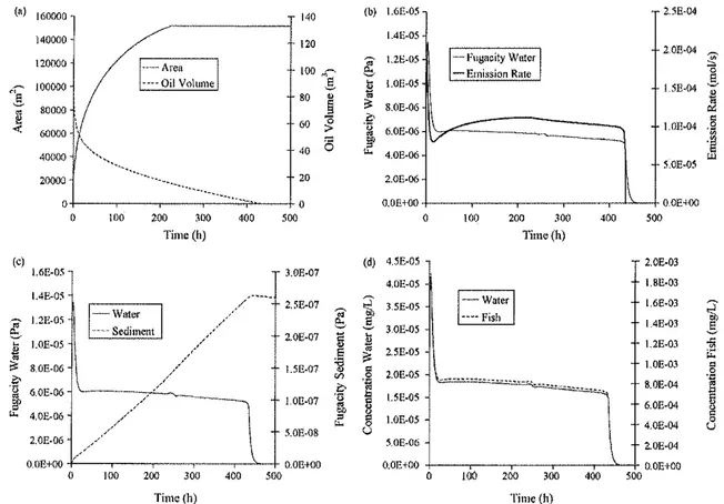
The surface oil slick area growth is shown in Fig. l(a). This area prescribes the dimensions of both evaluative compart-ments at a given time. The slick growth ceases as its thickness (13) (15) (14) where dVll2 DG2 = Z1l2di:

(9)

146

PROCESS SAFETY AND ENVIR.ONMENTAL PROTECTION 86 (2008) 141-r48

The advection process residence time can be calculated as;

The above expression shows that the advection residence time is implicitly a function of time during the slick area growth, and it increases with the square root of area. The advection residence time, averaged over the analysis period of

500h, is calculated as5 h,The reaction process residence time

(tresR2=l/kd is 346 h or ,-.".14.4 days,

water compartment shows a rapid decrease of its burden after the chemical input is stopped, but the sediment is slower to respond. Fig. l(c) thus indicates that the water compartment response is faster than that of the sediment compartment. This behavior stems from the fact that the water compartment has relatively high advection (DA2) and reaction (DRd pro·

cesses,

The group VZ/D provides valuable insight into the residence time associated with a transport process; the shorter the residence time, the more significant the process. The water-to-sediment transfer time for depletion of water through theD24process can be calculated as:

(17)

(1B)

53.3years

｛ＨｂｷｸｚＧ［ｾｳＩ

+

UDSZS]

tresA2=

ｖｾｾｅＲ

=

V;

ｪｾＺＨｴＩ

decreases to 0,01 em, resulting in a final area of 1.52 x lOS m2

at225 h.The oil volume curve is also shown in Fig. 1(a), with volume decreasing by the processes of evaporation and dispersion. The dispersion-emulsification formulation (as discussed in Section 2,1) eventually drives the residual oil (oil not evaporated) into the water column, thus giving the surface slick a finite lifetime. In the current example, the calculated surface slick lifetime is 435 h (...18 d).

The emission rate of naphthalene into the water column is presented as a function of time along with the water fugacity curve in Fig. 1(b).The chemical input to the water column becomes zero at 435 h, which correspondsto the surface slick lifetime. The shape of the emission rate curve depends on natural dispersion rate and oil slick volume (see Eq. (9f)). Oil slick volume decreases with time due to the evaporation and natural dispersion weathering processes, Assuming constant wind speed and oil-water interfacial tension, the variation of the product term (,ul/2ht 1 in Eq, (5) governs an increase or decrease of dispersion rate with time in the current simula-tions. Afterreachingits peak, approximately at1h (see Fig, tb), the emission curve starts decreasing, At an elapsed time of 16h a small increase in the emission rate curve is observed due to the higher dispersion rates,

The water and sediment fugacity curves are shown in Fig. l(c).Apeak in the water fugacity occurs at approximately

3h (which is very close to the input curve peak), whereas the sediment fugacity curve peaks at an elapsed time of447 h,The

(10)

147

(,) 160000 140 (b) L6E-05 2.5E-04 ]40000 ₁₂₀ 1.4E_05

ｉｾ

Fugacity Wlltcr

I

2,OE-04

ｾ

120000

ｾ

Un-OS 100 ",'-" _{Emission Rale} 100000

g

ｾ

I.OE-OS 1.5£-04

g

ｯｾ 80

• ｾ

§

_"

8,OE-06 ｾ 80000 ₆₀ '0 .i" ₁₁ <:

>-ｾ

6.OE-06 1.0E-04 60000 _V

...

--m

"",.",

..

_-,,--

40

[5

4.0E-06 40000

"'

5.0E-05 20000 20 2.0E_06 ＢＧｾＭＭ

..

0

.

-,- 0 O,DEtOa O,OE+oo 0 100 200 300 400 500 0 100 200 300 400 500 Time (h) Time (h)

(oJ (d) 4.5E-05 2,OE-03

L6E-05 3.0E-07 4,OE-05 I,BE-OJ IAE-05 ,/

ｾ

ｾＭｷＢＢ

I

1.68-03

i

2.5&07 3,5E-05

ｾ

J.2E-05 /'

ｾ

g

_3.0E-05 -_.- Fish IAB-03

" 2.0E-07

₁₁

_l!

_-Ii

j

LOE-05 ./ I.2E-03 E

•

2.5E-OS

'"

"

"" 1) 1.0E-03 § 8,OE-06 _/ I.5E-O?

'"

§ 2.0E-OS Ｎｾ

E'

// _;,;. _Ｎｾ _8.0E-04 _ｾ

•

6.0E-06 _{ＧｾＯ［ｾＭＭＭＭ} ·0 1.5E-05 _Ii gj' l,OE-O?

_a

_Il

6.0£-04

ｾ

""

4.0E-06 /

=

<3

1.0E-05 , / /

""

4.0E-04 5.0E-08 2.0£-06 / .' 5.0E-06 2.0£-04 /

O.OF,+()O a.OEtOO a.OEtOa O.OE+OO

(J ₁₀₀ ₂₀₀ ₃₀₀ ₄₀₀ ₅₀₀ ₀ ₁₀₀ ₂₀₀ ₃₀₀ ₄₀₀

_soo

Time (h) Timc(h)

Fig. 1 - Multimedia fate of Statfjord crude oil in the marine environment.

The last process associated with the water compartment is the growth process. The residence time for this pseudo transport process can be calculated as:

With respect to the time at which the slick growth ceases, i.e., [dA2/dt] ... 0, Eq, (19) shows that tresG2 ...00.This suggests

that the growth transport process is only important during the area growth regime, and should not be included in model Eqs, (12) and (13) outside the growth regime, In the current example, at an elapsed time of 2 h, the growth residence time has the same value as that ofthe averaged advection residence time. Further, the growth process residence time increases and at an elapsed time of 106 h its magnitude becomes equal to the value of the reaction process residence time. Once the slick growth is ceased (at ",,225 h), however, the growth process is no longer included in the fate modelling calculations.

The analysis suggests that the advection process has the lowest residence time, Hence, advection is the most important transport process in the water compartment.

In the case of sediment-to-water inter-media processes, the residence time is:

V

B2

2

B2

fdA,]

-1 ｾ tresG2=ｾ =Az

crt

=K 1V4/ 3 5.5years (19) (20)

time. The last transport process is the sediment burial and the associated residence time is:

hs

tresBur=

-u

_,,,

= 168 years (21)

The analysis shows that during the growth regime (up to 225 h), the growth process is the most important transport process in the sediment compartment.

Another important parameter is 2, which distributes the concentration between phases. A phase ofhigh 2 value (such as fish) absorbs a greater quantity of solute (organic chemical), resulting in higher concentrations while retaining a low fugacity. The converse is true for a phase having a low 2 value. The Z value for fish (26)is approximately 1.091 moVm3Pa; for

water, the value (22) is 0.024 mo1lm3_{Pa. This leads to fish}

concentrations which are2J22times higher than the water column concentrations. Fig. l(d) provides a comparison of fish and water column concentration profiles for the case study.

The predictive concentration profiles presented here are based on existing, validated oil weathering algorithms, and the multimedia fugacity-based model developed in the current work. Itshould be noted that further validation of the results would require laboratory/field dynamic concentra-tion measurements in coastal environmental media such as fish and ambient water.

5,

Conclusion

The reaction residence time (tresR2 = 1/k4 )is approximately 5200 h. The residence time for the sediment growth process is the same as that for the water compartment growth residence

The predicted trends of oil spill fate in a multimedia marine environment are in agreement with the theory of the fugacity

(11)

148

PROCESS SAfETY AND ENVIRONMENTAL PROTECTION 86 (2008) 141-148

modelling approach (e.g., the higher concentration trends in fish than in water are because of the higher Z value for fish). The study shows that the water compartment response to the chemical input is faster than the sediment compartment; this is expected because the advection process is present only in the water column. Further, the analysis shows that the

advection process displays the lowest residence time. We

therefore conclude that the proposed methodology effectively applies existing oil weathering algorithms, and the level IV fugacity model, to predict the fate of an oil spill in a marine environment. Extensions to the current work would include

further model validation by means of laboratory/field envir-onmental data and the inclusion of data uncertainty analysis,

Acknowledgements

The authors gratefully acknowledge the financial support of the Natural Sciences and Engineering Research Council (NSERC) of Canada under the Discovery and Strategic Grant Programs.

REFERENCES

API, 1999, Fate of spilled oil in marine waters (American Petroleum Institute), Publication Number 4691.

ASCE. 1996, State-of-the-art review of modelling transport and fate of oil spill,1Hydraul Eng, 122: 594-609.

Buchanan, I. and HurfDrd, N., 1988, Methods fDr predicting the physical changes in Dil spilt at sea, Oil Chem PoUut, 4(4): 311-328.

CONCAWE, 1983, Characteristics of petroleum and its behavior at sea. Report No. 8/83.

Exxon Corporation, 1985, Fate and effects of oil in the sea, Exxon Background Series.

Fay,l.A.1969, The spread of oil slicks on a calm sea, In D. P. Hoult (Ed.), oil on the Sea (pp. 53-63). NY: Plenum Press. Hoult, D.P., 1972, Oil Spreading on the sea. Annual Review of

Fluid Mechanics, Van Dyke (ed.), pp. 341-368,

Huda, M.K., Tkalich, P. and Gin, K.Y.H., 1999, A 3-D multiphase oil spill model, In Proceedings of the Conference, Oceanology International '99 Pacific Rim (pp. 143-150),

Mackay, D. 1991, Multimedia Environmental Models: The Fugacity Approach, (Lewis Publishers, USA).

Mackay, D., Buist, I., Mascarenhas, R. and Paterson, S., 1980, Oil Spill Processes and Models. (Environmental Protection Service, Environment Canada).

Mackay, D" JDy, M. and Paterson, S., 1983, A quantitative water, air, sediment interaction (QWASl) fugacity medel for describing the fate of chemicals in lakes, Chemosphere, 12: 277-291.

Mackay, D. and MacAuliffe, C,D., 1989, Fate efhydrocarbons discharged at sea, Oil Chern PoUut, 5(1): 1-20.

Mackay, D" Paterson,S, and Shiu, W.Y., 1992, Generic models for evaluating the regional fate of chemicals, Chemosphere, 24: 695-717.

MacLeod, M., Fraser, A. and Mackay, D., 2002, Evaluating and expressing the propagation of uncertainty in chemical fate and bioaccumulation models, Environ Texicol Chem, 21: 700-709.

Mooney,M.l.1951, The viscosity of a CDncentrated suspension of spherical particles, J Colloid Sci, 6: 162-170.

National Research Council (NRC). 1985, Oil in the Sea: Inputs, Fates, and Effects. (National Academy Press, Washington,

DC).

Reed, M. 1989, The physical fates component of the natural resource damage assessment model system, Oil Chem PoUut, 5(2-3): 99-123.

Sadiq, R., 2001, Drilling Waste Discharges in the Marine Environment: A Risk Based Decision Methodology. Ph.D. Dissertation (Faculty of Engineering, Memorial University of Newfoundland, Canada).

Sebastiao, P. and Soares, C.G., 1995, Modelling the fate of oil spills at sea, Spill Sci Technol Bull, 2:ＱＲＱｾＱＳＱＬ

Sebastiao, P. and Soares, C.G., 1998, Weathering of oil spills accounting for oil components, InR.Garacia-Martinez&C. A.Brebbia (Eds.), Oil and Hydrocarbon Spills, Modelling, Analysis and Control (pp. 63-72). Southampton, UK: WIT Press.

Stiver, W. and Mackay, D., 1984, Evaporation rates of spills of hydrocarbons and petroleum mixtures, Environ Sci Technol, 18(11): 834-840.

Sweetman,l.A.,Cousins, T.I., Seth, R., Jones, C.K. and Mackay, D., 2002, A dynamic level IV multimedia environmental model: application to the fate of polychlorinated biphenyls in the United Kingdom over a 60-year period, Environ Taxicol Chern, 21(5): 930-940.

Yang, W.C. and Wang, H., 1977, Modelling of oil evaporation in aqueous environment, Water Res, 11: 879-887.