HAL Id: hal-00905155
https://hal.archives-ouvertes.fr/hal-00905155
Submitted on 16 Nov 2013
HAL is a multi-disciplinary open access
archive for the deposit and dissemination of
sci-entific research documents, whether they are
pub-lished or not. The documents may come from
teaching and research institutions in France or
abroad, or from public or private research centers.
L’archive ouverte pluridisciplinaire HAL, est
destinée au dépôt et à la diffusion de documents
scientifiques de niveau recherche, publiés ou non,
émanant des établissements d’enseignement et de
recherche français ou étrangers, des laboratoires
publics ou privés.
Optimal Noise Maximizes Collective Motion in
Heterogeneous Media
Oleksandr Chepizhko, Eduardo G. Altmann, Fernando Peruani
To cite this version:
Oleksandr Chepizhko, Eduardo G. Altmann, Fernando Peruani. Optimal Noise Maximizes Collective
Motion in Heterogeneous Media. Physical Review Letters, American Physical Society, 2013, 110 (23),
pp.238101. �10.1103/PhysRevLett.110.238101�. �hal-00905155�
arXiv:1305.5707v1 [physics.bio-ph] 24 May 2013
Oleksandr Chepizhko, Eduardo G. Altmann, and Fernando Peruani
1
Department for Theoretical Physics, Odessa National University, Dvoryanskaya 2, 65026 Odessa, Ukraine
2
Max Planck Institute for the Physics of Complex Systems, N¨othnitzer Str. 38, 01187 Dresden, Germany
3
Laboratoire J.A. Dieudonn´e, Universit´e de Nice Sophia Antipolis, UMR 7351 CNRS , Parc Valrose, F-06108 Nice Cedex 02, France
(Dated: May 27, 2013)
We study the effect of spatial heterogeneity on the collective motion of self-propelled particles (SPPs). The heterogeneity is modeled as a random distribution of either static or diffusive obstacles, which the SPPs avoid while trying to align their movements. We find that such obstacles have a dramatic effect on the collective dynamics of usual SPP models. In particular, we report about the existence of an optimal (angular) noise amplitude that maximizes collective motion. We also show that while at low obstacle densities the system exhibits long-range order, in strongly heterogeneous media collective motion is quasi-long-range and exists only for noise values in between two critical noise values, with the system being disordered at both, large and low noise amplitudes. Since most real system have spatial heterogeneities, the finding of an optimal noise intensity has immediate practical and fundamental implications for the design and evolution of collective motion strategies.
PACS numbers: 87.18.Gh, 05.65.+b, 87.18.Hf
Most examples of natural systems, if not all, where collective motion occurs in the wild, take place in het-erogeneous media. Examples can be found at all scales. Microtubules driven by molecular motors form complex patterns inside the cell where the space is filled by or-ganelles and vesicles [1]. Bacteria exhibit complex col-lective behaviors, e.g. swarming, in heterogeneous en-vironments such as the soil or highly complex tissues such as in the gastrointestinal tract [2]. At a larger scale, herds of mammals migrate long distances travers-ing rivers, forests, etc [3]. Despite of these evident facts, little is known at both levels, experimental as well as the-oretical, about the impact that an heterogeneous medium may have on the self-organized collective motion [4]. For instance, most collective motion experiments have been performed on homogeneous arenas [4], from microtubules moving on fixed carpet of molecular motors [5], bacteria swarming on surfaces [6, 7], to marching locusts [8], and including fabricated self-propelled systems [9, 10]. Not surprisingly, most theoretical efforts have also focused on homogeneous media [4, 11], from the pioneering work of Vicsek et al. [12] to the detailed study of symmetries and large-scale patterns in self-propelled particle systems [13– 21], where the transition to collective motion is reduced to the competition between a local aligning interaction and a noise.
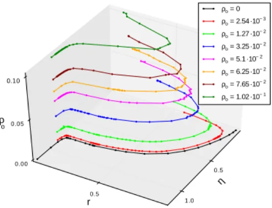
Here, we show through a simple model that the pres-ence of even few either static or diffusive heterogeneities changes qualitatively the collective motion dynamics. In particular, we find that there is an optimal noise ampli-tude that maximizes collective motion, while in an ho-mogeneous medium such an optimal does not exist, see Fig. 1. For weakly heterogeneous media ( i.e., low ob-stacle densities) we observe that the transition to col-lective motion exhibits a unique critical point below,
which the system exhibits long-range order, as in homo-geneous media. For strongly heterohomo-geneous media (high obstacle densities), we find on the contrary that there are two critical points, with the system being disordered at both, large and low noise amplitudes, and exhibit-ing only quasi-long-range order in between these critical points. The finding of an optimal noise that maximizes self-organized collective motion may help to understand and design migration and navigation strategies in either static or fluctuating heterogeneous media, which in turn may shed some light on the adaptation and evolution of stochastic components in natural systems that exhibit collective motion, for instance, concerning the bacterial tumbling rate.
Model definition.– We consider a continuum time
FIG. 1: (color online). Optimal noise amplitude. Order pa-rameter r as a function of noise strength η and obstacle den-sity ρo. Data corresponding to L = 140, Do= 0, and ρb= 1.
2
(a)
(b)
(c)
(d)
α
FIG. 2: (color online). (a) Details of the interaction between a SPP and an obstacle (η = 0.1). The dashed circle represents the interaction area, of radius Ro, the solid (black) curve corresponds to the particle trajectory, and α is the scattered angle. (b), (c) and (d) illustrate the different phases exhibited by the system with Do = 0 and ρo = 2.55 · 10−3 at the microscopic and macroscopic level: (b) clustered phase, η = 0.01 with order parameter r = 0.58, (c) homogeneous (ordered) phase, η = 0.3 with r = 0.97, and (d), band phase, η = 0.6 with r = 0.73. Insets correspond to snapshots of the entire system, where the red box inside them indicates the system area that is shown on main panel. For movies illustrating these phases see [23].
model for Nb SPPs moving in a two-dimensional space,
with periodic boundary conditions, of linear size L. SPPs interact among themselves via a (local) ferromagnetic ve-locity alignment as in [12]. Spatial heterogeneity is mod-eled by the presence of either fixed or diffusive obstacles. The new element in the equation of motion of the SPPs is given by the obstacle avoidance interaction by which SPPs turn away from obstacles whenever they are at a distance equal or less than Ro from them. The
imple-mentation of this rule is analogous to the archetypical (discrete) collision avoidance rule introduced in [22]. In the over-damped limit, we express the equations of mo-tion of the i-th particle as:
˙xi = v0V(θi) (1) ˙θi = g(xi) γb nb(xi) X |xi−xj|<Rb sin(θj− θi) + (2) + γo no(xi) X |xi−yk|<Ro sin(αk,i− θi) + ηξi(t) ,
where the dot denotes temporal derivative, xi
corre-sponds to the position of the i-th particle, θi to its
moving direction, and yk is the position of the k-th
obstacle. In Eq. (1), v0 is the active particle speed
and V(θ) ≡ (cos(θ), sin(θ))T. The interaction SPP-SPP
is defined by two parameters, the angular (relaxation) speed γb and the interaction radius Rb. Similarly, the
in-teraction SPP-obstacle is determined by γo and Ro. The
term nb(xi) (no(xi)) corresponds to the number of SPPs
(obstacles) that are located at a distance less or equal than Rb (Ro) from xi. In the second sum in Eq. (2),
the term αk,i denotes the angle, in polar coordinates, of
the vector xi− yk. The additive white noise is
char-acterized by an amplitude η and obeys hξi(t)i = 0 and
hξi(t)ξj(t′)i = δi,jδ(t − t′). The term g(xi) in Eq. (2)
controls the strength of the alignment with respect to
obstacle avoidance. For instance, g(xi) = [1 − Θ[no(xi)]]
with Θ[n] = 1 if n > 0, and 0 otherwise (switching rule), represents a scenario in which SPPs stop aligning in the presence of an obstacle, analogous to the hardcore re-pulsion rule introduced in [22]. We also consider a sim-pler scenario with g(xi) = 1 (no switching rule) where
particles never stop aligning to neighbors. Finally, ob-stacles are either fixed in space, or diffuse around with a diffusion coefficient Do. For simplicity, we initially fix
Rb= Ro= 1, γb = γo= 1, ρb= Nb/L2= 1, v0= 1, and
Do = 0 (with a discretization time ∆t = 0.1), and use
the switching rule. Other scenarios are discussed at the end.
If γ = 0, equations (1) and (2) define a system of non-interacting persistent random walkers. For γ > 0 and No= 0, Eq. (1) and (2) reduce to a continuum time
ver-sion of the Vicsek model (VM) [12] as proposed in [15]. It is for γ > 0 and No≥ 0 that we observe a completely
new behavior, since now the SPPs not only align among themselves but also avoid obstacles by turning away from them, with a characteristic turning time given by 1/γ. Fig.2illustrates the new aspects of the collective behav-ior, as well as a typical interaction between an obstacles and a SPP.
Optimal noise.– To characterize the macroscopic col-lective motion we use the following order parameter:
r = hr(t)it= h 1 Nb Nb X i=1 eiθi(t) it, (3)
where h. . .it denotes temporal average. Fig. 1 shows r
versus the angular noise η for various obstacle densities ρo= No/L2. The curve ρo= 0 corresponds to the
contin-uum time VM and as the noise amplitude η is decreased below a critical amplitude ηc1, r monotonically increases,
with r → 1 as η → 0 [4]. Here, we find that for ρo > 0
the scenario is qualitatively different and r exhibits a non-monotonic behavior with η. Moreover, we observe
that there is an optimal angular noise amplitude ηM at
which r reaches a maximum value. The relevance of this striking result is clear, due to the presence of a random distribution of obstacles, there exists an angular noise ηM that maximizes the collective motion. Notice that in
a simple model of particles driven in opposite directions it has been reported also the existence of an “optimal” noise, but in this case, contrary to what we report here, it freezes particle motion [25]. Fig. 1shows that the sys-tem is disordered, without exhibiting collective motion for η > ηc1. Collective motion and orientational order
increase as η is decreased from ηc1 to ηM.
Counterin-tuitively, decreasing η further hinders collective motion. If the density of obstacles ρo is large enough, we find
that unambiguously the system becomes fully disordered again but this time for η << ηM. The remarkable fact
is that there is a second, nonzero, critical angular noise amplitude ηc2 at large enough densities ρo.
Order-disorder transitions.– At low densities ρo, the
obtained numerical data suggests that for η ≤ ηc1 the
system exhibits long-range order (LRO). Increasing the system size, while keeping densities ρb and ρo constant,
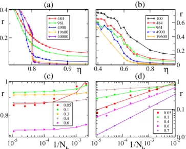
we observe that the transition becomes sharper with sys-tem size, Fig. 3(a). The transition at ηc1is accompanied
by the emergence of traveling high density structures, i.e., moving bands as observed in the VM [22]. Bands are observed only close to ηc1and at the optimal angular
noise ηM, they have always disappeared. On the other
hand, as the density of obstacles ρo is increased, bands
contain less particles, while the background density of SPPs increases, to the point that for large values of ρo
bands are no longer observed.
The existence of LRO implies that for a fixed η value, r should tend to an asymptotic value larger than 0 as the system size Nb goes to infinity. A useful way to estimate
this limit is to plot r as function of the inverse system size y, with y = 1/Nb, and extrapolate the behavior of
r when y → 0. This is shown in Fig. 3(c) for ρo =
2.55 · 10−3, where the solid curves correspond to fittings
with exponentials, i.e., r ∼ r∞(η) exp(A(η)Nb). Such a
scaling strongly suggests the existence of LRO for η < ηc1
at low ρo densities.
At higher densities, the system behavior is remarkably different. Fig. 3(b) shows that this time as the system size Nb is increased, the transition becomes smoother,
with the order parameter r decreasing with system size for all η value. We find that r obeys the following scaling with system size Nb:
r ∝ N−ν(η,ρo)
b , (4)
with ν(η, ρo) > 0, Fig. 3(d). Though this finding is
some-how reminiscent of an equilibrium Kosterlitz-Thouless (KT) transition [35], there are various fundamental dif-ferences. In first place, ν exhibits a non-monotonic be-havior with η, with a minimum at ηM, and ν = 1/2 at
0.8 0.9
η
0.2 0.4r
484 961 4900 19600 40000 0.4 0.6 0.8η
0 0.2 0.4 0.6r
100 484 961 4900 19600 10-5 10-41/N
10-3 b 1r
0.05 0.1 0.3 0.4 0.6 10-5 10-41/N
10-3 10-2 b 0.01 0.1 1r
0.05 0.1 0.4 0.6 0.7 0.8(a)
(b)
(c)
(d)
FIG. 3: (color online). Finite size scaling. Order parameter r vs. angular noise η for various system sizes Nb (color coded) for ρo= 2.55 · 10−3in (a) and ρo= 0.102 in (b). The scaling of r with system size Nbat fixed angular noise η (color coded) is shown in (c) and (d) for the obstacle densities correspond-ing to (a) and (b), respectively. The solid curves correspond to exponential fittings in (c) and power-laws in (d), which suggests the presence of LRO and QLRO, respectively.
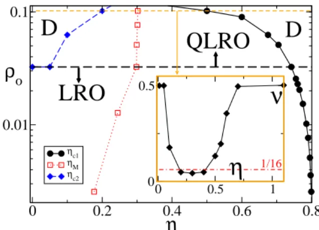
low and high η values, see inset in Fig. 5. Such a scaling corresponds to a fully disordered phase and indicates that in addition to ηc1, there is a second critical point ηc2for
low η values. In analogy with the KT transition, we de-fined ηc2 as the angular noise at which ν = 1/16. When
0 < ν < 1/16, we say that the system exhibits quasi-long range-order (QRLO). We stress that ν → 1/2 for nonzero η-values below ηc2, while ν reaches its minimum
value as η → ηM. In conclusion, the numerical data for
high obstacle densities ρo is consistent with QLRO for
ηc2 ≤ η ≤ ηc1. This means that at some intermediate
density ρ∗
o, which we roughly estimate around ρ∗o= 0.03,
there is a transition from LRO to QLRO.
Phases and physical interpretation.–We have seen that when ρo> 0 the order parameter r exhibits a maximum
at ηM. This means that we can find values of η to the
left and to the right of ηM that lead to the same value
of the order parameter r. The next logical question is whether we can say something regarding the state of the system for two different η-values that lead to the same value of r. To the right of ηM and close to ηc1 particles
organize into bands, Fig. 2(d). To the left of ηM and
close to ηc2, on the other hand, particles form very dense
clusters and freely moving particles are rarely observed. When these dense clusters collide with an obstacle, they often split into two or more fragments that are deflected away, see Fig. 2(b) and cluster phase movie in [23]. The new formed sub-clusters tend to move in uncorrelated directions. The dynamics is such that while a cluster
re-4 0 0.4 0.8 0 0.4 0.8
r
0.0025 0.005 0.015 0.025 0 0.4 0.80 0.4r
0.0625 0.102 0.11 0.13 0 0.4 0.8 0 0.4 0.8r
0.0025 0.0325 0.0625 0.102 0 0.4 0.80 0.4 0.8r
0.5 0.7 1.0 1.5 2.0(a)
(b)
(c)
(d)
D o=0.7 ρo=0.102 ρο= ρο= ρο= Do=η
η
η
η
no switching 2 int. zones
diffusing obst. diffusing obst.
FIG. 4: (color online). Robustness and generality of results. The same macroscopic behavior is observed in various varia-tions of the model. Data obtained with: (a) the no switching rule, i.e., g = 1, (b) two interacting zones (with Ro = 0.5, γo = 5 and Rb = γb = 1), while (c) and (d) correspond to diffusing obstacles, i.e., Do > 0. When parameters are not specified, they correspond to those used previously [24].
cruits particles and other clusters in between collisions, it breaks into very cohesive sub-clusters that move in differ-ent direction at each collision with an obstacle, with each sub-cluster experiencing a similar fate. As result of this process, the SPPs cannot form a highly ordered particle flow. But if η is increased, clusters are less cohesive and quickly spread out. This fast spreading of clusters allows sub-clusters to quickly reconnect and orientational order information is more efficiently distributed across the sys-tem, see Fig. 2(c). On the other hand, if we keep on increasing η, the noise ends up being too strong for the alignment strength γ and the system becomes disordered again.
Concluding remarks.– The same macroscopic behav-ior is observed in various SPP systems, which provides a strong evidence of the robustness and generality of the reported results. In particular, the existence of an opti-mal noise seems to be rooted in the fact that a certain amount of noise facilitates, in the presence of obstacles, the exchange of particles and information among clus-ters, which in turn promotes the emergence of large cor-relations in the system. Fig. 4 shows in (a) that the use of the “no switching” interacting rule between SPP-obstacles, i.e. g(xi) = 1, results in the same behavior,
in (b) that two interacting zones, for instance, a larger alignment zone with a smaller and faster repulsion zone, mimicking a hardcore repulsion as proposed in [22], do not alter the obtained results, and in (c) and (d) that the same macroscopic behavior is also observed with dif-fusing obstacles. This last observation is of particular relevance and extends the obtained results to fluctuating
0 0.2 0.4 0.6 0.8
η
0.01 0.1ρ
o ηc1 ηM ηc2 0 0.5 1 0 0.5D
LRO
D
QLRO
ν
η
1/16FIG. 5: (color online). Phase diagram. The solid black curve with dots corresponds to the critical noise amplitude ηc1and sets the boundary between a disordered (D) and an ordered phase. The ordered phase, below the horizontal dashed black line, corresponds long-range order (LRO), while below it, to quasi-long-range order (QLRO). Above the horizontal dashed black line, there is a second critical point, ηc2, indicated by the blue diamond curve. The dotted red curve indicates the position of the optimal noise strength ηM. The inset shows the behavior of the finite-size scaling exponent ν in Eq. (4) with the noise amplitude η for ρo = 0.102, which evidences the presence of the two critical points, see text and [24].
environments, which are of particular relevance in biolog-ical contexts such as the self-organization of microtubules inside the cell [1] or bacterial self-organization in hostile environments where either poisonous chemicals or bac-teria predators as lymphocytes diffuse around [2]. We notice that the stronger the diffusion Do, the weaker the
effect, with an increase of Do playing a similar role as a
decrease of ρo, Fig.4(d).
Our analysis reveals – up to the system sizes we man-age to explore – that the presence of heterogeneous me-dia leads to an unexpectedly complex phase me-diagram, as summarized in Fig.5. The most remarkable finding is the qualitative change of behavior – in a two dimensional sys-tem with continuum symmetry – from long-range order (LRO) and a unique critical point (ηc1), at low ρo, to
quasi-long-range order (QLRO) and two critical points (ηc1 and ηc2), at high ρo. Notice that QLRO occurs
with particles and interactions maintaining their polar symmetry and at finite densities, while QLRO in ho-mogeneous SPP systems has been found with particles and interactions exhibiting both apolar symmetry [33], as well as with metric interactions but in the zero density limit only [32]. Finally, there is a qualitative difference to previous “noise-induced order” examples [25–31]: the increase of order occurs here without requiring an exter-nal field or driving (and it is not induced by boundary conditions). A direct comparison with lane formation in systems with two populations of particles driven by an external field in opposite directions [25–28] reveals
fur-ther important differences [34], with the density of oppo-site moving particles playing the role of our noise and the strength of the external field as the inverse of our density of obstacles (cf. [26]).
In summary, we have reported about: 1) the existence of an optimal noise for self-organized collective motion in heterogeneous media, 2) a transition from LRO to QLRO in 2D, 3) QLRO in SPP systems at finite density with particles and interactions exhibiting polar symmetry, and 4) an example of noise-induced order without requiring an external field.
Numerical simulations have been performed at the ‘Mesocentre SIGAMM’ machine, hosted by Observatoire de la Cˆote d’Azur.
∗ Electronic address: [email protected]
[1] B. Alberts, D. Bray, J. Lewis, M. Raff, K. Roberts, and J. Watson, Molecular biology of the cell (Garland pub-lishing, 1994).
[2] M. Dworkin, Myxobacteria II (Amer Society for Micro-biology, 1993).
[3] R. Holdo, J. Fryxell, A. Sinclair, A. Dobson, and R. Holt, PLoS ONE 6, e16370 (2011).
[4] T. Vicsek and A. Zafeiris, Physics Reports 517, 71 (2012).
[5] V. Schaller, C. Weber, C. Semmrich, E. Frey, and A. Bausch, Nature 467, 73 (2010).
[6] H. Zhang, A. Be’er, E.-L. Florin, and H. Swinney, Proc. Natl. Acad. Sci. USA 107, 13526 (2010).
[7] F. Peruani, J. Starruss, V. Jakovljevic, L. Sogaard-Andersen, A. Deutsch, and M. B¨ar, Phys. Rev. Lett. 108, 098102 (2012).
[8] P. Romanczuk, I. Couzin, and L. Schimansky-Geier, Phys. Rev. Lett. 102, 010602 (2009).
[9] A. Kudrolli, G. Lumay, D. Volfson, and L. Tsimring, Phys. Rev. E 74, 030904(R) (2006).
[10] J. Deseigne, O. Dauchot, and H. Chat´e, Phys. Rev. Lett. 105, 098001 (2010).
[11] M. Marchetti, J.-F. Joanny, T. B. Liverpool, J. Prost, and R. A. Simha, arXiv p. 1207.2929 (2012).
[12] T. Vicsek, E. A. Czirok, E. B. Jacob, I. Cohen, and O. Shochet, Phys. Rev. Lett. 75, 1226 (1995).
[13] G. Gr´egoire and H. Chat´e, Phys. Rev. Lett. 92, 025702 (2004).
[14] F. Ginelli, F. Peruani, M. B¨ar, and H. Chat´e, Phys. Rev. Lett. 104, 184502 (2010).
[15] F. Peruani, A. Deutsch, and M. B¨ar, Eur. Phys. J. Special Topics 157, 111 (2008).
[16] F. Peruani, T. Klauss, A. Deutsch, and A. Voss-Boehme, Phys. Rev. Lett. 106, 128101 (2011).
[17] D. M. F. D. C. Farrell, M. C. Marchetti and J. Tailleur, Phys. Rev. Lett. 108, 248101 (2012).
[18] A. Gopinath, M. Hagan, M. Marchetti, and A. Baskaran, Phys. Rev. E 85, 061903 (2012).
[19] J. Toner and Y. Tu, Phys. Rev. Lett. 75, 4326 (1995).
[20] J. Toner and Y. Tu, Phys. Rev. E 58, 4828 (1998).
[21] S. Ramaswamy, R. A. Simha, and J. Toner, Europhys. Lett. 62, 196 (2003).
[22] G. Gr´egoire and H. Chat´e, Phys. Rev. Lett. 92, 025702 (2004).
[23] See supplementary material for movies. .
[24] Param.: Rb= Ro= γb= γo= 1, ρb= 1, v0= 1, Do= 0.
[25] D. Helbing, I.J. Farkas, and T. Vicsek, Phys. Rev. Lett. 84, 1240 (2000).
[26] J. Chakrabarti, J. Dzubiella, and H. L¨owen, Phys. Rev. E 70, 012401 (2004).
[27] J. Dzubiella, G.P. Hoffmann, and H. L¨owen, Phys. Rev. E 65, 021402 (2002).
[28] J. Chakrabarti, J. Dzubiella, and H. L¨owen, Europhys. Lett. 61, 415 (2003).
[29] A. Rosato et al., Phys. Rev. Lett. 58, 1038 (1987).
[30] J.A. Gallas, H.J. Herrmann, and S. Sokolowski, Phys. Rev. Lett. 69, 1371 (1992); J. Phys. II France 2, 1389 (1992).
[31] Y. Limon Duparcmeur, H.J. Herrmann, and J.P. Troadec, J. Phys. I France 5, 1119 (1995).
[32] F. Ginelli and H. Chat´e, Phys. Rev. Lett. 105, 168103 (2010).
[33] H. Chat´e, F. Ginelli, and R. Montagne, Phys. Rev. Lett. 96, 180602 (2006).
[34] The comparison requires a suitable Galilean transforma-tion. Notice that the external field breaks the symmetry.
[35] J. M. Kosterlitz and D. J. Thouless, J. Phys. C: Solid State Phys. 6, 118 (1973).