Assessing the criticality of germanium as a by-product

Assessing the Criticality of Germanium as a

By-product

by

Nagisa Tadjfar

Submitted to the Department of Materials Science and Engineering

in partial fulfillment of the requirements for the degree of

Bachelor of Science in Materials Science and Engineering

at the

MASSACHUSETTS INSTITUTE OF TECHNOLOGY

June 2017

@

Massachusetts Institute of Technology 2017. All rights reserved.

Author

...

Signature redacted

if

Departilent of Materials Science and Engineering

May 5, 2017

Certified by..

redacted...

Elsa A. Olivetti

Assistant Professor of Materials Science and Engineering

Thesis Supervisor

7

Accepted by ...

MASSACHUSETTS INSTITUTE OF TECHNOLOGY

JUN

0

5 2017

Signature redacted

Geoffrey Beach

Professor of Materials Science and Engineering

Chairman, Undergraduate Thesis Committee

Acknowledgments

I would like to thank my incredibly supportive and helpful thesis advisor, Professor Elsa Olivetti for her guidance throughout the development of this work. Professor Olivetti provided insightful comments at every step in the research and writing of this thesis, and I appreciate all that I have learned about industrial ecology from her. I would also like to thank Xinkai Fu for all his help and guidance throughout the course of this thesis. He put in an enormous amount of time to teach me about his research and help me learn how to drive this thesis on my own. His hard work and thoughtfulness in how he approaches research has been truly inspirational.

I am also very grateful for the entire Materials Science and Engineering faculty

and staff at MIT for all that I have learned from them throughout my time in the department. Lastly, I am incredibly lucky to have had a wonderful class of peers, the entire Materials Science and Engineering Class of 2017, and I am thankful to have learned so much from them and to call them my friends.

Assessing the Criticality of Germanium as a By-product

by

Nagisa Tadjfar

Submitted to the Department of Materials Science and Engineering on May 5, 2017, in partial fulfillment of the

requirements for the degree of

Bachelor of Science in Materials Science and Engineering

Abstract

Although germanium production is currently nowhere near its supply potential, many sources cite germanium, a by-product material produced primarily from zinc and coal, as a critical metal. Current methods for assessing criticality include frame-works that rely on geopolitical risk metrics, geological reserves, substitutability, and processing limitations during extraction among others but there is a gap in under-standing the complex supply and demand dynamics that are involved in the market for by-products. This thesis addressed this gap by assessing the supply risk of ger-manium using an econometric framework to generate estimates of price elasticities. Annual world production and price data of years 1967 - 2014 for germanium was used to construct supply and demand models in order to obtain estimates for the price elasticities of supply and demand. Ordinary least squares (OLS) regression was used on an autoregressive distributed lag (ARDL) model for both supply and demand. The supply model was constructed with price, zinc production, and 5-year interest rate as shifters along with lag terms for germanium production, germanium price, 5-year interest rate, and zinc production. The adjusted R2 was 0.761 and the long term supply price elasticity was found to be 0.05 with an upper bound of 0.7 and a lower bound of -0.6 indicating that germanium supply is price inelastic. In a simi-lar fashion, a demand model was constructed with two structural breaks accounting for fundamental changes in the market structure in 1991 and 2003, along with lag terms for germanium production, germanium price and antimony price. The adjusted

R2 _{value for the demand model was 0.683 and the price elasticity was 0.05 with an}

upper bound of 1 and a lower bound of -1 indicating that demand, too, is price in-elastic. This creates an added risk for supply shortages, adding to the criticality of germanium. However, the stabilizing behavior of its carriers, coal and zinc, reduce the likelihood of an actual shortage. This type of analysis improves upon existing methods and can lead to more accurate quantified estimates for long-term criticality. Thesis Supervisor: Elsa A. Olivetti

Contents

1 Introduction

2 Methodology

2.1 Partial Equilibrium of Supply and Demand . . . 2.2 Supply and Demand Shifters . . . .

2.3 Autoregressive Distributed Lag (ARDL) Model

2.4 Regression Analysis . . . .

3 Model

3.1 Identifying Supply and Demand Shifters . . . .

3.2 Identifying Structural Breaks . . . .

3.3 Testing for Price Endogeneity . . . .

3.4 Testing for Autocorrelation . . . .

4 Results 5 Conclusion 5.1 Future W ork . . . . 7 13 13 16 18 18 20 . . . . 20 . . . . 24 . . . . 26 . . . . 27 29 35 36

List of Figures

1-1 The breakdown of end-use of germanium worldwide in 2015. . . . . . 8

1-2 The supply curve of a by-product can be segmented into a by-product region that is inelastic (AC) and an elastic main product (DF) region of the curve (cf. Frenzel (2016, Fig. 2)). . . . . 9 1-3 The logarithm of current germanium production is shown along with

supply potential from zinc as well as total supply potential from coal. 11

2-1 Demand and supply in three time periods (adapted from Stock & Wat-son 2011) . . . . 14 2-2 Equilibrium prices and quantities from 12 periods appear as a

scatter-plot (adapted from Stock & Watson 2011) . . . . 15 2-3 The logarithm of germanium quantity is plotted against price in the

time period 1967-2014. . . . . 16 3-1 List of supply and demand shifters that were statistically significant

before adding lag terms and structural breaks. . . . . 21

3-2 The Bayesian information criterion for different numbers of structural

breaks is shown. . . . . 24

3-3 The two structural breaks chosen are shown in dashed lines at 1991

and 2003. ... ... 25

3-4 Autocorrelation was tested for in the supply model. The dashed blue lines indicate the margin within which autocorrelation is not significant. 27

3-5 Autocorrelation was tested for in the demand model. The dashed blue

List of Tables

3.1 Summary of OLS results on supply for germanium. . . . . 22

3.2 Summary of OLS results on demand for germanium . . . . 23

4.1 Summary of coefficients of final model for supply of germanium. . . 31

4.2 Summary of coefficients of final model for demand of germanium. . 32

4.3 Long-term supply and demand elasticities along with the upper and lower bounds for germanium. Both supply and demand were found to be inelastic. . . . . 34

Chapter 1

Introduction

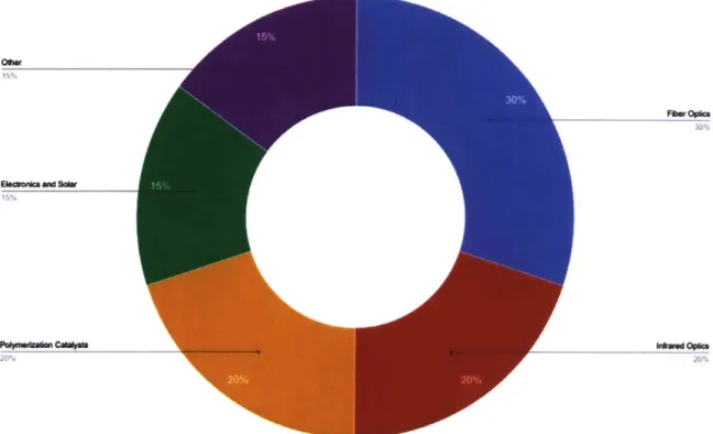
Germanium is a vital mineral with widespread global applications in a broad range of items prevalent in day-to-day life as well as military and defense equipment. Germanium is a high-refractive index, intrinsic semiconductor with unique properties such as IR transparency, all of which have led to its use in electronic and optical de-vices among the others aforementioned. Germanium is also used as a polymerization catalyst for manufacturing polyethylene terephthalate. The worldwide consumption of germanium in 2015 and its breakdown by product is given in Figure 1-1 (USGS,

01W

E~Fbwk OWac

15%

Pa&~uma~~m~CInfred Opncs

20%

Figure 1-1: The breakdown of end-use of germanium worldwide in 2015.

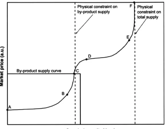
Recently, there has been much discussion about the future availability of gernium; in 2010 the European Commission identified germanium as a 'critical' raw ma-terial, meaning it is a material with economic importance with non-negligible future supply risk (European Commission, 2010). A large part of why germanium is often deemed critical is due to the nature of its production. Germanium is one of several minerals that are produced as by-products. Furthermore, 100% of its global pri-mary production is currently obtained in the form a by-product (Nassar, 2015). This means that rather than being mined for its own sake, it is produced as a consequence of major materials. Specifically, by-products do not influence the profit-maximizing level of production (Lovik, 2016). Because of this behavior, price increases of several orders of magnitude are required to break away from being constrained by the carrier production as shown in Figure 1-2 adapted from Frenzel et al. (Frenzel, 2016)

4,

8

4

C By-product supply curve C

B

A

Supply (quantityltIme)

Figure 1-2: The supply curve of a by-product can be segmented into a by-product region that is inelastic (AC) and an elastic main product (DF) region of the curve

(cf. Frenzel (2016, Fig. 2)).

By-products are often considered to be critical because of this added supply risk compared to minerals produced as main products. Because of shared production costs with the carrier, there is often a large difference between the cost of producing a mineral as a main product and the cost of producing that same mineral as a by-product. This can create large shifts in the total supply curve during the switch from by-product to a main product produced on its own, resulting in large price shifts (Redlinger, 2016). By-product materials have often undergone large price fluctuations following increases in demand motivated by technology. For instance, between 2006 and 2007, ruthenium experienced a ninefold price increase due to growing demand from hard disk drives (Nassar, 2015). This indicates that supply of a by-product may be inelastic with price; given sufficient change in demand, prices may increase drastically without an actual increase in quantity supplied, adding to supply risk

physical constraint on F Physical

>y-product supply constraint on total supply

E

and thus criticality of a given mineral. This risk may be further worsened by inelastic demand for the mineral. These shifts in the supply curve of the by-product result from demand shocks in the carrier market, according to the "by-product effect" (Afflerbach, 2014).

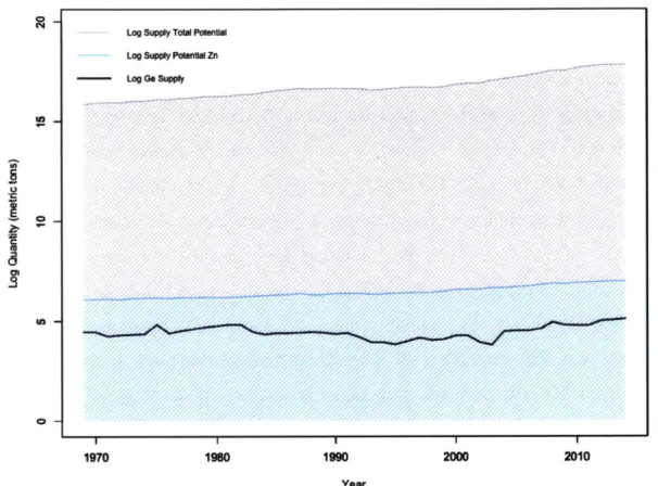
In assessing the criticality of germanium as a by-product, it is natural to begin with a comparison of current supply and supply potential to examine how far histor-ical production has been and current production is from the supply potential. The two major germanium deposits are Sulphidic lead-zinc deposits and high-germanium lignite deposits. Therefore, germanium is mostly produced from zinc-smelter residues and high-germanium coal ashes (Frenzel, 2013). It is estimated that 60% of germa-nium extraction is originated from zinc and 40% from coal fly ash. Thus, germagerma-nium is a by-product of two carriers, both zinc and coal and its supply potential is con-strained by their reserves. Recovery efficiency was assumed to be 100% in order to eliminate processing constraints and focus on direct physical constraint from carrier. Figure 1-3 below shows cumulative germanium supply potential form both zinc and coal plotted against time along with the actual germanium production at each year. It is clear that germanium production is nowhere near the supply potential and would require orders of magnitude of change in order to be even close to exceeding supply potential. However, germanium is special because it has two primary carriers rather than just one. It is worthwhile to examine whether these two carriers, zinc and coal interact in any way that either exacerbate or mitigate future supply risk.

Various criticality assessments of germanium among other 'critical' raw materi-als have been conducted. The European Commission used a geopolitical-economic framework which consisted of quantifying the political stability of major produc-ers, the geographical concentration of production, substitutability and recycling rate of the material and combining this information into a Herfindahl-Hirschmann-Index (European Commission, 2010). Their analysis also included measures that might be taken by countries with weak environmental performance in order to protect the en-vironment which may affect supply. Lovik et al. computed supply potential using carrier production, extraction limitations as well as material loss rates and

recy-Lo Supply Totol Pabntl - LogoqpyPoeuiZn - Log Go Suppy -

7/"

// / / ///////&/f// /////////// // A#0N N/A7/1//////A#f/ ~t1/// W7// / /;7/// // // W// ~J4JM/ /J/fM Mif / 7/ '/ J//// " ////AWSAdM/FM 7/ /////nezrz/0//m#WM0 wzm 1970 1960 1990 2000 2010 Yewr

Figure 1-3: The logarithm of current germanium production is shown along with supply potential from zinc as well as total supply potential from coal.

cling (Lovik, 2016). Frenzel et al. conducted a study on the geological availability of germanium, concluding larger reserves than previously estimated (Frenzel, 2013). However, geological availability alone cannot fully capture the criticality of a mate-rial that has complex market dynamics as a result of its by-product status. Other criticality and supply risk assessments that have been carried out include the work of Frenzel et al. on gallium, where supply potential was modified from the traditional 'reserves'-based definition to take into account statistical distributions in different raw materials as well as marginal costs of production of the by-product (Frenzel, 2016). While these results argued for the case that geological availability cannot completely describe the criticality for by-products, there is a gap in existing literature as to how to better address this problem and incorporate the complicated supply-demand

dy-namics of by-products. Existing literature considers only geopolitical risks associated

with producing countries or approaches supply risk with an emphasis on processing

limitations.

A more comprehensive, econometrics-based approach on how material supply

re-acts to fluctuations in price that reflect changes in demand are necessary to fully assess supply risk. The purpose of this thesis is to address this gap by constructing a model of supply and demand elasticity for germanium. Understanding the drivers of its supply and determining whether supply is price inelastic will ultimately im-prove upon the current framework for evaluating the criticality of a given mineral and understanding its supply risk. Because of the special behavior of byproducts, it is expected that the supply of germanium would be inelastic. The more inelastic the price elasticity of supply, the higher the risk of future supply shortages, despite large

supply potentials. However, because germanium is unique in that it has two carriers rather than one, it is also of interest to explore how coal and zinc production relate,

as this may have stabilizing effects on the supply of germanium, lowering supply risk

Chapter 2

Methodology

2.1

Partial Equilibrium of Supply and Demand

Partial equilibrium (PE) analysis was used to model interactions in the germa-nium market under the balance between supply and demand. This balance is called

equilibrium in standard economic theory and is defined as the price and quantity at

which the quantity supplied equals the quantity demanded. The quantity supplied and demanded will vary until the two equal, converging to this equilibrium point (Perloff, 2011).

This is visualized using supply and demand curves in Figure 2-1, where the equi-librium points are the intersections between the black supply curves and the blue demand curves. The equilibrium points at three time periods are labelled Eq.1, Eq.2, and Eq.3 respectively.

Price _Eq.2 -4% 4% 4% 4% 4% 4% 4% - - - -- -

4%

~~

i

.j~..

~ 4% - 4% __________ Eq. 3 4% 4%. *1% * 4% 4% 4% 4% 4% 4% 4% 4% Eq. 1 Quantity

Figure 2-1: Demand and supply in three time periods (adapted from Stock & Watson 2011)

The sensitivity of quantity demanded to price is called price elasticity of demand and the sensitivity of quantity supplied to price is the price elasticity of supply. In a simple model, as shown in Figure 2-1, the supply elasticity is represented by the slope of the supply curve. Similarly, the demand elasticity is the slope of the demand curve. More formally, elasticity can be described by:

P dQ

Q

dP (2.1)

In each time period in Figure 2-1, both the supply and demand curves are shifting due to factors other than price. In each of these periods, the factors shifting the curves can also be different. The market characteristics that shift supply and demand curves

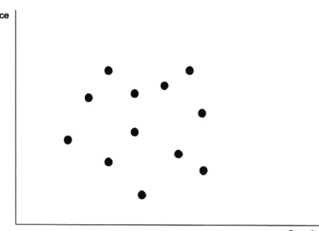
in such ways are called supply shifters and demand shifters. Given only production and price data, the data would be in the form of a scatterplot as shown in Figure 2-2.

Price 0 S S S S S Quantity

Figure 2-2: Equilibrium prices and quantities from 12 periods appear as a scatterplot (adapted from Stock & Watson 2011)

This motivates the need for identifying factors that only affect supply and not demand as well as factors that only affect demand and not supply. Once such pa-rameters have been isolated, they can be used to model supply and demand curves. These shifts in the supply curve in ways that are uncorrelated to the demand cause the equilibrium points to fall on the same demand curve. In this way, the demand and supply curve can be isolated, enabling us to correctly estimate supply elasticities on the same supply curve and demand elasticities on the same demand curve.

2.2

Supply and Demand Shifters

Supply curves may shift in ways uncorrelated to demand and demand curves may shift in way uncorrelated to supply. In order to account for such shifts, we introduce supply shifters into the model. Similarly, demand shifters are also introduced. In addition to market supply and demand shifters, additional structural breaks were considered to account for stepwise changes in the market. Figure 2-3 shows the trends in the natural logarithm of germanium production and price over the years

1967-2014. 'a (3 Sn 0~ 0 CE, 1970 1980 1990 Year 2000 W) 06 U) &i 2010

2-3: The logarithm of germanium quantity 1967-2014.

is plotted against price in the time

When specifying a regression model, it is assumed that any assumptions apply to all the observations in our sample. It is straightforward, however, to test the hypothesis that some or all of the regression coefficients are different in different

sub-- Log Supply Go

Log Price Go

Figure period

sets of the data. As Figure 2-3 suggests, the germanium market was significantly less volatile, with price moving together with quantity prior to 1990 and was quite volatile thereafter. The period between 1990 - 2000 is peculiar as price and quantity move in opposite ways. These non-negligible stepwise shifts observed in the data can be rationalized by historical events that occurred. This is likely due to the increase in demand due to IR devices as well as growth in germanium use as a catalyst, while the National Defense Stockpile (NDS) began sales due to a lowered target, pushing down price despite growing demand. In the mid 2000's, the price and quantity begin moving together again with a steady upward climb similar to the pre-1990's. It there-fore seems unlikely that the same regression model would apply to both periods and it is worth considering the use of structural breaks to account for this segmentation of the data. Structural breaks can be identified in the data, that is, specific points in time where a "shift" occurred can be identified and incorporated into the model. There are generally two approaches to accounting for structural breaks:

1. The first method is to run regressions on the subintervals rather than

run-ning a combined regression.

2. The second method is to add dummy variables that behave as step-function shifters in the quantity of germanium and then run a regression over the entire time period

The second approach was taken in this thesis, such that step-function shifters in the quantity of germanium were added to the model and an overall regression was used to compute the supply and demand elasticities for 1967-2014. This is justified

by the fact that the germanium dataset is fairly small, so reducing it into smaller

sections would run the risk of making the results less meaningful as long term val-ues. Thus, structural breaks were inserted in the form of either demand or supply shifters depending on the context of the historical changes in the market structure. As explained in chapter 3, for the case of germanium, both structural breaks were identified as demand shifters and included in the demand model as such.

2.3

Autoregressive Distributed Lag (ARDL) Model

Both supply and demand were tested for autocorrelation, to determine if there is significant dependence on previous values of the variables. The relationships between supply, demand, and the covariates were modeled using an autoregressive distributed lag (ARDL) model where the potential quantities depend linearly on their previous values and the effects of the regressors are distributed over time. Thus, supply and demand were modeled in the form:

Q P k Z

Qfi = C+-q + E 2,iPt-p , +

T,(2.2)

q=O p=O i=1 z=O

Q P k Z

= C" +

5

7"Qtq + E I1,pPtp +

5

f2,i,zZi- + (2.3)

q=O p=O i=1 z=O

where Qt represents world production of germanium in period t, Pt represent the price at time t, and Zi,t is a set of control variables representing various supply shifters and demand shifters, C is a constant, and Et represents the error term. The index i denotes the number of shifters for supply and demand each, the indices p, z, and q represent the specific lag term up until the lag orders P,

Q,

and Z at the top of the sum. The lag order for each variable was determined for the model.

2.4

Regression Analysis

Ordinary least squares (OLS) was used to perform backward stepwise regression to select the most statistically significant shifters. Once all of the significant shifters

for both supply and demand are identified, the Bayesian information criterion (BIC) of the vector autoregressive (VAR) model was used to select the optimal lag order,

1. A new dataset including only significant shifters and all lag terms up until the lag

order for each variable was created and the subset of variables that maximizes the adjusted R2 of the model was chosen. Finally, coefficients were estimated from the best model, from which long run supply elasticity e, and demand elasticity ed can be computed.

Data for the variables was collected from multiple databases and reports such as United States Geological Survey (USGS) historical statistics and US Board of Governors of the Federal Reserve System and all analysis was carried out using R.

Chapter 3

Model

3.1

Identifying Supply and Demand Shifters

Several supply and demand shifters were proposed based on the standard methods for a commodity as well as market specifics for germanium. The parameters were first introduced based on the market context for germanium and then verified for statistical significance afterwards. Interest rate was introduced as a supply shifter based on Hotelling's rule for exhaustible resources which states that a commodity stored underground can be treated as a capital asset (Hotelling, 1931). Hence, 1-year, 5-year, and 10-year interest rates in the United States were proposed, and the interest rate with the largest correlation with germanium production was chosen. It is also natural that metal supply will be affected by industrial production activities, which motivated the use of an industrial production index as a potential supply shifter. Three such indices were proposed, the Organization for Economic Co-operation and Development Industrial Production Index (OECD IP) , G7 IP, and US IP. Similarly

to the interest rates, the industrial production index with the highest correlation with germanium production was then chosen to be included in the model. Finally, in the context of by-product metal supply, primary supply of both zinc and coal were introduced.

On the demand side, business cycle and growth indicators were chosen, specifi-cally, S&P 500 and world GDP are both common demand shifters used in such models

and were therefore introduced. Prices of major substitutes for germanium were also included. Silicon is a commonly used, less-expensive alternative to germanium in elec-tronic applications and antimony is a substitute of germanium dioxide in the catalysis of the polymerization of polyethylene terephthalate (USGS, 2015). Finally, time was taken to be a common shifter between both supply and demand. In constructing the model, parameters measured in $ such as germanium price, world GDP and S&P

500, silicon (Si) price , and antimony (Sb) price were deflated using the 2010 GDP

implicit price deflator to remove distortions in the economic variables due to inflation. It was also assumed that indium (In) and cadmium (Cd) demands will not affect Zn supply and thus germanium supply, since Zn is also a carrier for In and Cd. This is based on the fact that they both have extremely low value ratios, making them very insignificant in comparison to Zn for a Zn producer such that they would not be able to drive up Zn production in any way. Tables 3.1 and 3.2 show the variables after running an ordinary least squares regression, identifying the most statistically significant variables. Notice that price needed to be forced in both for the supply and demand; this may be somewhat of an indication'of inelasticity. Thus, the variables that were included in the supply and demand prior to testing for autocorrelation and structural breaks are summarized in Figure 3-1 below:

Demand ShiMers

[& ]

World GDP Silicon Price Antimony Price Supply Shifters USIP G7IP OECD 5yr interest ZnCoal

P ~~production qatt

Figure 3-1: List of supply and demand shifters that were statistically significant before adding lag terms and structural breaks.

Table 3.1: Summary of OLS results on supply for germanium. Dependent variable: Ge quantity Ge price Zn production OECD IP 5y Interest Rate Coal production Constant 0.034 (0.110) 3.485*** (0.754) 0.005 (0.010) 0.082*** (0.020) 0.995 (0.619) 0.000 (0.030) Observations 48 R 2 _0.701 Adjusted R2 _0.665 Residual Std. Error 0.211 (df = 42) F Statistic _{19.661*** (df = 5; 42)}

Table 3.2: Summary of OLS results on demand for germanium. Dependent variable: Ge quantity Ge price World GDP S&P 500 Sb price Si price Constant 0.093 (0.119) 0.073 (0.563) -0.354** (0.146) 0.283** (0.106) 0.096 (0.301) 0.000 (0.040) Observations 48 R2 0.489 Adjusted R2 _0.428 Residual Std. Error 0.275 (df = 42) F Statistic 8.046*** (df = 5; 42)

3.2

Identifying Structural Breaks

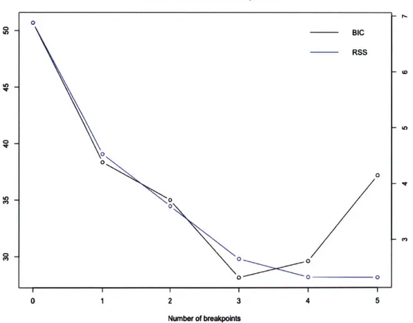
Simultaneous estimation of multiple breakpoints within the time series data was found using an implementation of an algorithm in the package 'strucchange'. This uses the F statistic (Chow test) to test for whether it is justifiable for coefficients in different regions to be different. The F statistic will have some critical value, and if the computed F statistic, which is obtained from the sum of squares of the different functional forms, exceeds that value, the hypothesis that the two coefficients are the same is rejected. The optimal number of breakpoints to include was identified such that the Bayesian information criterion (BIC) estimator was minimized. Figure 3-2 shows that the BIC estimator for the germanium data set is minimized at three breakpoints.

BIC and Residual Sum of Squares

0 2 3 3 4 - Ce) 5 Number of breakpoints

Figure 3-2: The Bayesian information criterion for different numbers of structural breaks is shown. 0 BIC RSS 0 0 0o 00 O\O I 1

However, from a historical standpoint, only two major events come to mind within the 1967 - 2014 time period:

1. The dot-com bubble in the 1990s that led to an artificial surge in construction

of fibre optic networks

2. The move from sealed bids to negotiated bids in the germanium market effective June 11, 2001 (Mining Journal, 2001a)

Thus, despite the fact that three breakpoints may be statistically preferable, two structural breaks were used in the model, one for each of the above two events. In fact, when specifying for two structural breaks, the results shown in Figure 3-3 agree well with the historical context. The data was partitioned into three regions, before

1991, between 1991 and 2003, and after 2003 as indicated by the vertical dashed lines.

0~ *16~~ a-In 1970 1980 1990 Yewr 2000 2010 Figure 3-3: 2003.

The two structural breaks chosen are shown in dashed lines at 1991 and

Two structural breaks were therefore identified in years 1991 and 2003, which align well with historical changes in the market that occurred, namely the dot-com bubble in the 1990s as well as the move from sealed bids to negotiated bids in the germanium market in 2001 whose effects could have been felt more in 2003, were added. These effects were added to the demand model in the form of two dummy variables, D1 and D2 that take on the value 1 at 1991 and then at 2003 respectively

representing upward vertical shifts:

0, t < 1991.

Di = (3.1)

1,

t >1991.

D2t<2003 (3.2)

1, t ;> 2003

3.3

Testing for Price Endogeneity

It is worth noting that in the above models, price is assumed to be exogenous. A parameter is only exogenous if it is uncorrelated with the error terms. An exogenous supply shifter only affects the demand indirectly through its effect on price. Similarly, an exogenous demand shifter does not affect supply except through its effect on price and can be used as a valid instrument for price in the supply equation. This is not always true; the coefficient of price may not just be capturing the effect of price on demand or supply and an additional indirect change may be included in which case the use of a two-step least squares method is more appropriate. Price endogeneity in germanium was therefore tested for using the demand and supply shifters as instruments, both of which were found to be valid instruments correlating with price using the F-test. However, using the Wu-Hausman test for both supply and demand, price was found to be exogenous.

3.4

Testing for Autocorrelation

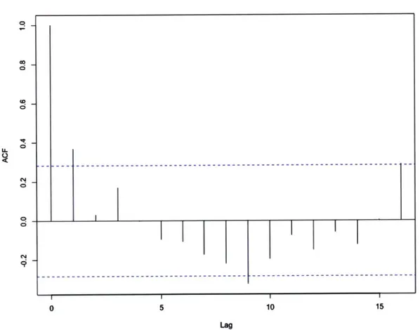
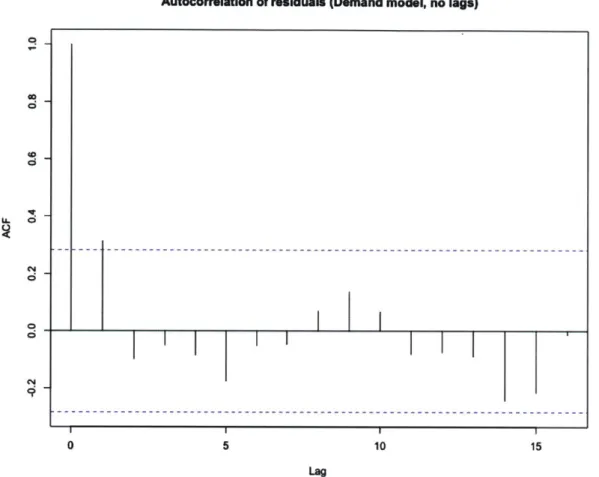
As discussed in Chapter 2, it is common for models of commodity production to include lag terms for the variables associated in the model. The models using the variables found to be statistically significant as shown in Figure 3-1 were tested for autocorrelation. Figures 3-4 and 3-5 show the results for the test for autocorrelation. The blue dashed lines indicate the margins within which autocorrelation is insignifi-cant. The horizontal axis represents the lag order and the vertical axis represents the

autocorrelation function corresponding to each lag term.

AutocorrelatIon of residuals (supply model, no lags)

C 0 0 a 0 5 10 15 Lag

Figure 3-4: Autocorrelation was tested for in the supply model. The dashed blue lines indicate the margin within which autocorrelation is not significant.

----Autocorrelation of residuals (Demand model, no lags) qt LL0

CII

I

I

II I 0 5 10 15 Lag

Figure 3-5: Autocorrelation was tested for in the demand model. The dashed blue lines indicate the margin within which autocorrelation is not significant.

The vertical bar corresponding to lag order 1 lies above the blue dashed line threshold in both the supply and demand models, indicating that autocorrelation up to the first lag term was detected in both. The most statistically significant shifters along with the appropriate lag terms up to one lag order that maximized adjusted R2 were selected for the final autoregressive models. The combination of all those variables that maximized the adjusted R2 _{value was chosen for supply and demand.}

Chapter 4

Results

The final models for supply and demand obtained using the statistically significant variables, combination of lag terms up to lag order 1 that maximized adjusted R2 values, that included dummy variables as demand shifts are provided in equations 4.1 and 4.2:

ln(Qd) = !31ln(Pt)+/321n(Pt-)+-ln(Qti)+,yD1,t+7y2D2, +d3ln(Ps,t--1)+e (4.1)

ln(Q") = ailn(Pt) + a2ln(Pt-1) + 7y1ln(Qzn,t) + 72ln(Qzn,t-1) + -ln(Qti)

t _(4.2)

+4lnI(5yJRsb,t) + 3

5f(5yIRSb,t_1) + 6ts

It is worth commenting on the fact that since the subset of the statistically sig-nificant shifters and their lag terms combined were chosen to maximize the adjusted

R2_{, certain parameters dropped out, which is expected since adjusted R}2 _{takes into}

account not only the improvements in a model but the number of predictors it has. It may seem surprising that the price of antimony (or in fact its first lag term, that is the price of antimony of the previous year) is the only demand shifter other than

the structural breaks to remain in the demand model. However, qualitatively this is also not unreasonable. There is no strong dominance of a single usage for germanium, with its consumption being fairly evenly distributed across infrared, optical fibers, so-lar, etc. The largest fraction is only 30% so germanium consumption as a catalyst for PET production, which takes up 20%, is in fact quite a significant part of germanium usage. Historically, PET catalysis was also an even larger part of germanium usage, with up to 25% in 2011 and antimony is the dominant material used as a catalyst for PET occupying 90% of the market. Furthermore, within the infrared space, germa-nium does not have good direct substitute meaning that antimony price can indeed influence germanium prices. Granger causality tests were also run to further quanti-tatively examine the effect of antimony on germanium. Antimony prices were found to granger cause germanium quantity, but not the other way around. This makes sense since Sb production is approximately 1000 times that of germanium production and its usage is mainly (>99%) in ceramics and glass, ammunition, flame retardants such that the usage for which germanium and antimony are substitutes more heavily influences germanium.

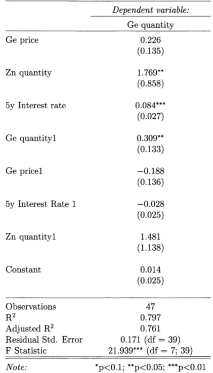
Since price was found to be exogenous, an ordinary least squares regression was run on these models to obtain estimations on each coefficient. The coefficients and standard errors for the final supply and demand models as shown in equations 3.3 and 3.4 are summarized in Table 4.1 and Table 4.2. On the supply side, the coefficient for zinc quantity was found to be positive, which is expected as an increase in zinc production from the previous year should in fact have a positive relationship with germanium production this year. On the demand side, we find that the coefficients also agree with intuition, the coefficient of antimony price is positive, as is expected of a substitute. As antimony prices increase, we would expect germanium production to increase due to an increase in demand for germanium which would now be a more attractive catalyst for PET production.

Table 4.1: Summary of coefficients of final model for supply of germanium. Dependent variable: Ge price Zn quantity 5y Interest rate Ge quantityl Ge pricel 5y Interest Rate 1 Zn quantityl Constant Ge quantity 0.226 (0.135) 1.769** (0.858) 0.084*** (0.027) 0.309** (0.133) -0.188 (0.136) -0.028 (0.025) 1.481 (1.138) 0.014 (0.025) Observations 47 R 2 0.797 Adjusted R2 _0.761 Residual Std. Error 0.171 (df = 39) F Statistic 21.939*** (df = 7; 39) *p<0.1; **p<0.05; ***p<0.01 Note:

Table 4.2: Summary of coefficients of final model for demand of germanium. Dependent variable: Ge quantity Ge price Dl D2 Ge quantity 1 Ge price 1 Sb price 1 Constant 0.239 (0.152) -0.200** (0.096) 0.211* (0.122) 0.481*** (0.111) -0.213 (0.160) 0.121* (0.071) 0.069 (0.043) Observations 47 R 2 0.725 Adjusted R2 _0.683 Residual Std. Error 0.197 (df = 40) F Statistic 17.543*** (df = 6; 40) Note: *p<0.1; **p<0.05; ***p<0.01

The coefficients for all the shifters were computed along with their standard er-rors. The long-term supply and demand elasticities were calculated using the formulas shown in equation 4.3, which are derived from the formal definition of price elasticity in equation 2.1.

P P

e' = O and ed = O (4.3)

q=1 q=1

The long-term price elasticity of supply is then e = 0.301988) .05 up to one

significant figure. The long-term price elasticity for demand is also computed in this way and is equal to ed = (0.239-0.213) _1-0.481 = 0.05

-Because the long-term supply and demand elasticities are functions of several variables extracted from the regression, each with standard errors of their own, prop-agation of error was used to accurately convey the error in our result. Additionally, due to the small data size, the white estimator correction was applied to the standard errors computed. The formula for computing the error in a general function q(x, ... , z)

of several variables is:

6q = + Oz2 6)(x (4.4)

where 6x is the random uncertainty corresponding to variable x.

These standard errors were used to generate confidence intervals for the elastic-ity estimates found above. Table 4.3 summarizes the long-term supply and demand elasticities computed along with the upper and lower bounds of the estimates. At

0.05 for both supply and demand, within the confidence interval of 95% they are both

found to be price inelastic.

Table 4.3: Long-term supply and demand elasticities along with the upper and lower bounds for germanium. Both supply and demand were found to be inelastic.

95% confidence Supply Demand

Lower Bound -0.6 -1 Upper Bound 0.7 1

Long-term Elasticity 0.05 0.05

The presence of two major carriers in the case of germanium, zinc and coal, may mitigate or exacerbate supply risk depending on how they interact. If zinc production and coal production are highly correlated, for instance, then supply risk in the future, depending on the trajectories of coal production, may be high.The Pearson correlation of the differences of historical time series data for zinc and coal production in years

1967-2014 was found to be 0.32. Though a negative correlation would have been

ideal to mitigate supply risk, because 0.32 is still relatively small, the existence of two carriers stabilizes the production of germanium, reducing its criticality.

Chapter 5

Conclusion

Autoregressive supply and demand models for germanium were constructed using

USGS data from 1967-2014 using supply and demand shifters as well as two

struc-tural breaks for the demand model. Both supply and demand were found to be price inelastic, both having the value 0.05. This increases the supply risk of germanium because inelastic supply suggests that even if prices were driven up by technological breakthroughs, for instance, that shift demand for germanium, the supply will not respond, leaving a shortage. Furthermore, inelastic demand worsens the situation, as demand will not decrease even in the case of extreme price increases. This certainly adds to the criticality of germanium. However, because germanium has two carriers rather than one primary carrier, and the correlations of the differenced time series data for zinc and coal production are not highly correlated, there is a stabilizing ef-fect, reducing supply risk and therefore criticality. Such econometrics-based analysis of supply and demand elasticities as well as understanding what factors drive supply and demand for by-product metals is an important enhancement to the current frame-work used to analyze by-product criticality. Supply elasticity can also be used as a criticality indicator from a market perspective. Though current methods for quantify-ing by-product criticality include metrics such as geopolitical risk, extraction process limitations, and geological reserves, these methods lack an economic component for supply risk. Supply elasticity allows for comparison between various by-products and lends itself to further analysis for policymaking as it is useful for predicting how the

market would respond to increased recycling for instance, as discussed in Future Work below.

5.1

Future Work

Future work includes constructing predictive models for germanium, zinc, and coal to try to predict if an intersection of demand and supply potential will hap-pen and evaluate the situations and assumptions would cause that. As the existing germanium-based products such as military vehicles, fiber optic cables, and solar cells age and eventually are no longer used, a surge in recycled germanium from the recov-ered end-of-life products is expected in the coming years (USGS, 2014). Currently, the global average end-of-life functional recycling rates of germanium is estimated to be less than 1% (Graedel, 2011). Industrial materials like germanium do not nec-essarily have a demand cap, meaning that an increase in supply in a substitute, in the form of increased secondary supply, can shock the system and influence prices of both primary and secondary materials. This influence can be studied by constructing displacement models based on primary supply and demand elasticities of germanium and determining cross price elasticities depending on the quality of the secondary material (Zink, 2015). Thus, the demand and supply elasticities calculated in this work can be used to investigate the displacement of germanium and to assess how an increase in secondary supply can affect primary supply and prices depending on how comparable secondary germanium would be to primary germanium. Including recy-clability and using the supply and demand elasticities to analyze the displacement of germanium can therefore enhance the model and better inform policymakers.

Moreover, the approach taken in this thesis provides an additional metric to im-prove upon existing methods for estimating the criticality of by-products and allow for quantitatively predicting consequences for supply shortages. A similar approach may be used to generate estimates for price elasticities for supply and demand of other by-product metals such as indium or selenium, which may lead to better assessments of their long-term criticality.

Bibliography

[1] Afflerbach, P., Fridgen, G., Keller, R., Rathgeber, A. W., & Strobel, F. (2014).

The by-product effect on metal markets - New insights to the price behavior of minor metals. Resources Policy,42, 35-44.

[2] Commission E (2010) Critical raw materials for the EU. Report of the Ad-hoc Working Group on Defining Critical Raw Materials. Brussels, Belgium

[3] Frenzel, M., Ketris, M. P., & Gutzmer, J. (2013). On the geological availability of

germanium. Mineralium Deposita,49(4), 471-486.

[4] Frenzel, M., Ketris, M. P., Seifert, T., & Gutzmer, J. (2016). current and future availability of gallium.

On the Resources Policy, 47, 38-50. doi:10.1016/j.resourpol.2015.11.005

[5] Graedel, T. E., Allwood, J., Birat, J., Buchert, M., Hagelken, C., Reck, B. K., .. .

Sonnemann, G. (2011). What Do We Know About Metal Recycling Rates? Jour-nal of Industrial Ecology, 15(3), 355-366. doi:10.1111/j.1530-9290.2011.00342.x

[6] Hotelling, H. (1931). The economics of exhaustible resources. The Journal of

Po-litical Economy, 39(2), 137-175.

[7] Lovik, A. N., Restrepo, E., & Mller, D. B. (2016). Byproduct Metal

Availabil-ity Constrained by Dynamics of Carrier Metal Cycle: The Gallium?Aluminum Example. Environmental Science & Technology,50(16), 8453-8461.

[8] Mining Journal, (2001)a, Minor metals in May: Mining Journal, v. 336, no. 8637,

[9] Nassar, N. T., Graedel, T. E., & Harper, E. M. (2015). By-product metals are

technologically essential but have problematic supply. Science Advances, 1(3).

[10] Perloff, J. M. (2011). Microeconomics. Harlow: Pearson Education.

[11] Redlinger, M., & Eggert, R. (2016). Volatility of by-product metal and mineral

prices. Resources Policy,47,69-77.

[12] Stock, J. H., & Watson, M. W. (2015). Introduction to econometrics. Boston, MA: Pearson.

[13] United States Geological Survey. Antimony (2015). Retrieved February 2017

from https://minerals.usgs.gov/minerals/pubs/commodity/antimony/mcs-2015-antim.pdf

[14] United States Geological Survey. Germanium (2014). Retrieved April 2017 from https://minerals.usgs.gov/minerals/pubs/commodity/germanium/mybl-2014-germa.pdf

[15] United States Geological Survey. Germanium (2015). Retrieved January 2017

from https://minerals.usgs.gov/minerals/pubs/commodity/germanium/mcs-2015-germa.pdf

[16] Zink, T., Geyer, R., & Startz, R. (2015). A Market-Based Framework for

Quan-tifying Displaced Production from Recycling or Reuse. Journal of Industrial Ecol-ogy, 20(4), 719-729.