Publisher’s version / Version de l'éditeur:
HVAC and R Research, 19, 5, pp. 513-535, 2013-07-23
READ THESE TERMS AND CONDITIONS CAREFULLY BEFORE USING THIS WEBSITE.
https://nrc-publications.canada.ca/eng/copyright
Vous avez des questions? Nous pouvons vous aider. Pour communiquer directement avec un auteur, consultez la
première page de la revue dans laquelle son article a été publié afin de trouver ses coordonnées. Si vous n’arrivez pas à les repérer, communiquez avec nous à PublicationsArchive-ArchivesPublications@nrc-cnrc.gc.ca.
Questions? Contact the NRC Publications Archive team at
PublicationsArchive-ArchivesPublications@nrc-cnrc.gc.ca. If you wish to email the authors directly, please see the first page of the publication for their contact information.
Archives des publications du CNRC
This publication could be one of several versions: author’s original, accepted manuscript or the publisher’s version. / La version de cette publication peut être l’une des suivantes : la version prépublication de l’auteur, la version acceptée du manuscrit ou la version de l’éditeur.
For the publisher’s version, please access the DOI link below./ Pour consulter la version de l’éditeur, utilisez le lien DOI ci-dessous.
https://doi.org/10.1080/10789669.2013.803400
Access and use of this website and the material on it are subject to the Terms and Conditions set forth at
Tubular daylighting devices: development and validation of a thermal
model (1415-RP)
Laouadi, Abdelaziz; Saber, Hamed H.; Galasiu, Anca D.; Arsenault, Chantal
https://publications-cnrc.canada.ca/fra/droits
L’accès à ce site Web et l’utilisation de son contenu sont assujettis aux conditions présentées dans le site LISEZ CES CONDITIONS ATTENTIVEMENT AVANT D’UTILISER CE SITE WEB.
NRC Publications Record / Notice d'Archives des publications de CNRC:
https://nrc-publications.canada.ca/eng/view/object/?id=84c6f686-0188-4586-b77e-e34ea21d8764 https://publications-cnrc.canada.ca/fra/voir/objet/?id=84c6f686-0188-4586-b77e-e34ea21d8764
Tubular Daylighting
Devices-development and validation of a thermal
model (1415-RP)
Abdelaziz Laouadi
*, Hamed H. Saber, Anca D. Galasiu, and Chantal Arsenault
*NRC Construction
National Research Council of Canada
1200 Montreal Road, Ottawa Ontario, K1A 0R6, Canada Tel: (613) 990 6868. Fax: (613) 954 3733
* Corresponding author. Email: aziz.laouadi@nrc-cnrc.gc.ca
Abstract
This paper presents the development and validation of a simplified model to compute the thermal characteristics (Solar Heat Gain Coefficient (SHGC) and thermal conductance (U-factor)) and surface temperatures of Tubular Daylighting Devices (TDDs). The model takes into account the three modes of heat transfer: conduction, convection and surface-to surface radiation. A one-dimensional heat conduction model is applied to TDD glazing layers. The convective heat transfer from TDD surfaces to their adjacent air spaces uses existing correlations for natural flows in enclosed air cavities and free stream air spaces. A zonal model, in which the pipe air space is divided into a number of thermally stacked zones, is used to predict the vertical average temperature distribution in the air cavity and wall surface of pipe. Thermal radiation exchange among surfaces uses the formulation of the form factor applied to the aforementioned zonal model. An iterative sequential procedure proposed to solve for the temperature distribution in TDD glazing layers and air cavities. The U-factor predictions of the simplified model are compared with the NFRC certified product rating measurement data and detailed CFD simulations. Four TDD products are simulated under the NFRC standard rating conditions for the residential (insulation at ceiling level) and commercial (insulation at roof level) settings. The temperatures of the TDD glazing layers and vertical temperature distribution inside the pipe air space are also compared with the CFD simulations. The results show that the U-factor predictions of the simplified model are in good agreement with the measurement data and CFD simulations, within a maximum deviation of 15% for both the residential and commercial rating conditions.
Introduction
Tubular Daylighting Devices (TDDs) are systems that collect and channel daylight from building roofs into deep interior spaces. A typical TDD system consists of three parts: a collector located on the roof to gather sunbeam light and diffuse skylight, a hollow pipe that channels the collected light downwards, and a ceiling diffuser that spreads light indoors. The collector is usually made of single or multiple transparent plastic domes, and may include geometries or some optical devices to enhance the light output of the device, especially at low sun altitude angles. The pipe can be straight rigid, elbowed rigid, or flexible, and is typically constructed from an aluminum sheet with a highly reflective interior lining. Materials with reflectivity of 99% are commercially available. The pipe may be fully or partially insulated at the ceiling or roof level to suit a particular building type. The diffuser is hemispheric or planar with single or double translucent (opal) or clear prismatic glazing.
TDDs have initially emerged as alternatives to conventional skylights to deliver daylight without the undesired solar heat gains, and to cover areas that are not usually covered by windows and skylights. Nowadays, TDDs compete with conventional skylights, particularly in commercial and residential buildings. Many big box retailers regularly use TDDs in their corporate design standards (Deru and MacDonald, 2007; Torcellini et al., 2007). TDDs are also encouraged or mandated, particularly in commercial buildings. For example, the recent building code (Title 24, Part 6) of the California Energy Commission (CEC, 2011) requires certain commercial building types to be daylit using diffusing skylights and TDDs. Building rating tools such as LEED (USGBC, 2011) assign point credits to daylit buildings. To meet the increasing need for high standards of building-energy efficiency and glare-free indoor environments, TDD technologies, focusing mainly on the optical efficiency of its components, have been rapidly and continuously evolving over the past two decades. However, due to the product’s complexity and rapid development, prediction of the daylighting and thermal performance of TDDs has always been a difficult task. Building designers and engineers and TDD manufacturers lack reliable and accurate calculation methods and design tools that would allow them to accurately predict the energy performance of installed TDDs, to show compliance with building-energy codes, and to rate existing and/or innovative TDD products.
Recognizing the high market penetration of TDDs, researchers over the world have extensively addressed the daylighting performance of TDDs (for example: CIE, 2006; Kocifaj et al., 2010; Goudey et al., 2010; Laouadi et al., 2013a,b,c). There are, however, very limited studies on the thermal performance of TDDs. The National Fenestration Rating Council (NFRC) attempted before to develop a simple model to compute the U-factor of TDDs
(Curcija, 2001). In a subsequent study, Architectural Testing Inc. (ATI), through an NFRC-funded project, designed a new horizontal hot box facility and carried out measurement of U-factor of several types of TDDs to validate the simple model. The test facility consisted of three major spaces: (a) a bottom guarded metering chamber housing the diffuser of the test specimen; (b) an intermediate attic or plenum space housing the pipe of the test specimen; and (c) a top weather chamber housing the collector of the test specimen. The comparison results of U-factor found out that there were significant differences between the measurement and predictions of the simple model (ATI, 2009). This led NFRC to adopt the physical testing procedure NFRC 102/201-2010 (NFRC, 2010a,b) to measure the thermal characteristics (thermal conductance (U-factor) and Solar Heat Gain Coefficient (SHGC)) of TDDs. The physical testing procedure of ATI has not, however, been publically peer-reviewed, or compared with other procedures such as detailed CFD simulations.
Objectives
This paper is a part of the ASHRAE research project 1415-RP: Thermal and lighting and performance metrics of tubular daylighting devices. The aim of the project is to develop detailed and validated algorithms to compute the thermal and lighting performance metrics of TDDs. This paper focuses on the prediction of the thermal performance of TDDs to complement previous work on the prediction of the optical performance of complex TDDs (Laouadi et al., 2013a,b,c,d). The specific objectives of this paper are:
To develop a simplified thermal model to compute the thermal characteristics (U-factor, and SHGC) and surface temperatures of TDDs under a variety of environmental operating conditions in commercial and residential buildings.
To conduct CFD simulation for selected commercially available TDD products.
To validate the simplified thermal model by comparing its results with the measurement-based certified product rating data and CFD simulations.
Model Development
Heat transfer in a typical TDD system is a complex phenomenon. All modes of heat transfer are involved and coupled to each others, namely: conduction through TDD material layers, surface-to-surface radiation, and convection in enclosed air cavities and free-stream air spaces adjacent to TDD surfaces. Detailed and accurate
calculation of heat transfer in TDDs using a multi-dimensional CFD approach is not practical since it involves prohibitive calculation times. The model under consideration uses a simplified, but accurate enough approach to compute the thermal performance of TDDs in a reasonable time frame so that the model can be integrated in existing fenestration design software and building energy computer simulation tools. Details of the model follow.
GEOMETRY DESCRIPTION
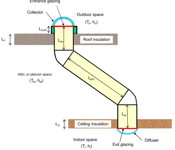
Figure 1 shows a schematic representation of a typical TDD system. A typical TDD system consists of a multi-pane domed collector, a single flat glazing at the pipe entrance surface, a hollow pipe with roof and ceiling elbows, a single flat glazing at the pipe exit surface, and a multi-pane ceiling diffuser. Insulation may be placed at the ceiling level, or at the roof level, or at both levels, and may cover the whole pipe length. The upper pipe section may project above the roof line in the curb space to accommodate proper water-proof flashings. The outdoor, and attic (for residential buildings) or plenum (for commercial buildings) conditions are applied to the TDD sections above the roof line, and in the attic or plenum space, respectively. The indoor conditions are applied to the ceiling diffuser.
Figure 1: Schematic representation of a typical TDD system
Lcurb Lri Lpu Lpm Lpl Lci (Tat, hat) Indoor space Roof insulation
Attic, or plenum space
(To, ho) (Ti, hi) Ceiling insulation Outdoor space Collector Entrance glazing Diffuser Exit glazing
ASSUMPTIONS
The following assumptions are considered. 1. Thermal properties of layers are constant.
2. Each glazing layer is assumed solid with effective thermal radiation and thermal properties.
3. Heat transfer through a glazing layer is by one-dimensional heat conduction. Effect of edge-of-glazing on heat transfer is, thus, not accounted for.
4. Thermal radiation may be uniformly absorbed along a layer thickness, or at the layer boundary surfaces, depending on its transparency to radiation.
5. Solar radiation is uniformly distributed over TDD glazing surfaces, and uniformly absorbed along the thickness of transparent layers. This assumption relates to the crude assumption (#3). It holds when a surface is
uniformly exposed to solar radiation. TDD surfaces may, however, be under non-uniform distribution of solar radiation, particularly for the domed collector glazing at low sun altitude angles, and the concentration of sunlight at the diffuser surface (hot spots). The combined effects of non-uniform distribution of solar radiation and edge-of-glazing will result in multi-dimensional heat flows. In this case, the computed one-dimensional temperatures may be regarded as surface-averaged temperatures.
6. Temperatures of the pipe surface and its air cavity are assumed uniform (averaged) over the pipe cross-section plane, but may vary along the pipe length.
7. Outdoor, attic or plenum, and indoor air spaces are at uniform temperatures.
Subject to the foregoing assumptions, the heat balances at the collector, pipe and ceiling diffuser will be made to cover heat conduction, convection, and surface-to-surface radiation.
ENERGY BALANCES AT COLLECTOR
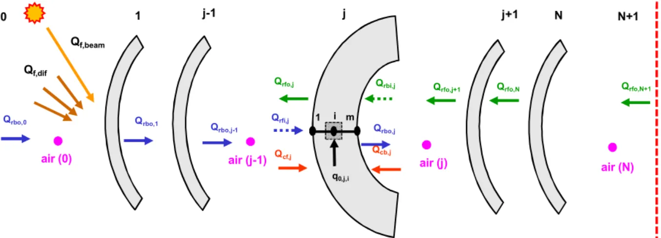
TDD collectors exchange heat to the adjacent environments by all modes of heater transfer. Figure 2 shows the distribution of the radiative and convective heat flows through a multi-layer domed collector. The collector is bounded by the exterior environment and the glazing layer at the pipe entrance surface.
Consider a collector with (N) glazing layers. The layers and air spaces are numbered in an increasing order from the outside to the inside environments. In this regard, layer j = 0 indicates the outside environment and layer j = N+1 indicates the glazing at the pipe entrance surface. Layer j = 1 is exposed to sunbeam and sky diffuse radiation, and thermal radiation from the outside environment, whereas the internal layer j = N is exposed to only thermal radiation.
Figure 2: Radiative and convective heat flows through a multi-layer domed collector (note that layer (j) is enlarged to show the internal nodal grid)
Conduction heat transfer
By referring to an isolated layer (j) of Figure 2, the transient energy balance at internal node (i) within the layer is expressed in a spherical coordinate system by the following relation (Siegel and Howell, 2002):
∙ , = ∙ , − , , + , , + , , (1)
Where:
cj : effective specific heat of layer j (J/kg/K, Btu/lb/°F)
kj : effective thermal conductivity of layer j (W/m/K, Btu/h/ft/°F)
qr,j,i : radiation flux density at node i of layer j (W/m2, Btu/h/ft2)
qsol,j,i : net absorbed solar radiation per unit volume at node i of layer j (W/m3, Btu/h/ft3)
q0,j,i : heat generation per unit volume at node i of layer j (W/m3, Btu/h/ft3)
r : radial coordinate at node i of layer j (m, ft) Tj,i : temperature at node i of layer j (K, °F)
t : time (s)
j : effective density of layer j (kg/m3, lb/ft3)
The net absorbed solar radiation per unit volume (qsol,j,i) at node (i) is expressed as follows:
, , = , ∙ + , , ∙ ∙ ∆ ,/ , (2)
Where:
Qbeam : beam solar radiation flux incident on the TDD surface (W, Btu/h)
Qdif : diffuse solar radiation flux incident on the TDD surface (W, Btu/h)
Vj,i : volume of the elemental volume associated with node i of layer j (Vj,i= Sj,i∙rj,i) (m3, ft3)
rj,i : radial thickness of the elemental volume associated with node i of layer j (m, ft)
j,i : absorption coefficient per unit thickness of layer j at node i for the incident beam solar radiation (m-1, ft-1)
d,j,i : absorption coefficient per unit length of layer j at node i for the incident diffuse solar radiation (m-1, ft-1).
j 1 N Qrfi,j Qcf,j Qcb,j Qrfo,j q0,j,i Qrbo,j Qrbi,j i Qrfo,N Qrbo,1 1 m air (j) air (j-1) Qf,beam Qf,dif j-1 j+1 Qrfo,j+1 Qrbo,j-1 N+1 Qrfo,N+1 Qrbo,0 0 air (N) air (0)
The nodal solar absorption coefficients (j,i) may be calculated based on the layer solar absorptance (ABj; more
details are available in Laouadi et al., 2013b). In the absence of a photovoltaic energy conversion, one may assume that the solar radiation is uniformly absorbed along the layer thickness (Lj). In this case, the nodal solar absorptance
coefficients are equal to the layer solar absorptance divided by its thickness (j,i= ABj/Lj).
The nodal radiation flux density (qr,j,i) is a complex quantity to calculate. A proposed approach is to formulate
the nodal radiation flux density in terms of the effective emission (absorption) coefficient of a layer medium, its nodal emissive power and the incident thermal radiation from all directions. In this approach, the layer medium is assigned a nodal effective emission (absorption) coefficient, which may be pre-calculated based on a detailed thermal radiation model for the layer medium. The effective emission coefficient indicates the portion of the black body energy emitted per unit length, which exits from the layer boundary surfaces. By virtue of the Kirchhoff’s law (Siegel and Howell, 2002), the effective absorption and emission coefficients are equal. The effective radiation properties depend on the medium geometrical details, and may vary along the layer thickness. In this approach, the gradient of the radiation flux density is expressed as follows:
− , , = , ,∙ , , ,∙ ,
, − , , + , , ∙ ,; i = 1 to m (3)
Where:
Ej,i : black body emissive power at node i of layer j (W/m2, Btu/h/ft2)
Qrbi,j : thermal radiation flux incident on the back surface of layer j, given by equation (23) (W, Btu/h)
Qrfi,j : thermal radiation flux incident on the front surface of layer j, given by equation (22) (W, Btu/h)
Sj,i : cross-section area of the elemental volume associated with node i of layer j (m2, ft2)
b,j,i : back effective emission coefficient per unit length at node i of layer j (m-1, ft-1)
f,j,i : front effective emission coefficient per unit length at node i of layer j (m-1, ft-1)
For layers, which are fully transparent to thermal radiation, the emission and absorption of thermal radiation may occur along the layer thickness. In this case, the nodal emission coefficients may be assumed equal to the layer effective emissivity (eff,j) divided by the thickness (rj,i) of its elemental volume (j,i= eff,j/rj,i).
Following the definition of the optical characteristics of TDDs (Laouadi et al., 2013b), the solar radiation incident on the TDD surface is expressed in terms of the internal pipe cross-section area as follows:
= ∙ ; = ∙ (4)
Ibt : solar beam irradiance incident on a tilted TDD pipe entrance surface (W/m2, Btu/h/ft2)
Idt : solar diffuse irradiance incident on a tilted TDD pipe entrance surface (W/m2, Btu/h/ft2)
Spi : internal area of the pipe entrance surface (m2, ft2)
Numerical method
Equation (1) is nonlinear and, therefore, does not admit a closed-form analytical solution. A suitable numerical method should, thus, be used to obtain the temperature distribution within the layer medium. Integrating equation (1) over an elemental spherical control volume associated with the internal nodal points (i = 2 to m-1), one obtains the following equation:
. , ∙
, = , ∙ − , ∙ + , , + , , − , , ∙ , (5)
Where Sj,i-1/2 and Sj,i+1/2 are surface areas at the interfaces between nodes i and i-1 and nodes i and i+1,
respectively.
By replacing the derivatives in equation (5) by their central differentiation forms, equation (5) may be further reduced for a uniform nodal grid (nodes are uniformly spaced) within a layer to the following:
. ∆∆ , − , ∙ , = , ∙ , − , − , ∙ , − , + , , + , , − , , ∙ ∆ ∙
, (6)
Where Toldis the nodal temperature calculated at the previous time step (t –t).
By re-arranging the terms, equation (6) becomes: − 1 +∆ , . , + . ∆ ∆ + 2 . , − 1 − ∆ , . , = ∆ ∆ , + ∆ . , , + , , − , , ; i = 2 to m − 1 (7)
Equation (7) is subject to the convective boundary conditions at nodes i =1 and m (Figure 2). A heat balance at the elemental control volume of a half width (r/2) associated with the boundary node i = 1 will result in the following equation:
,
, = , − ∙ , ∙ + , , + , , − , , ∙ , (8)
Where Qcf,jis the convective heat flux exchanged between the adjacent air space and the front boundary surface
, = ℎ, ∙ , , − , (9) Where:
hc,j-1 : convection average film coefficient of the air space of index (j-1) adjacent to node (i = 1) of layer (j)
(W/m2/°C, Btu/h/ft2/°F)
Sj,i=1 : surface area associated with node (i = 1) of layer (j) (m2,ft2)
Ta,j-1 : average temperature of the adjacent air space of index (j-1) (°C,°F)
By replacing the derivative in equation (8) by its central differentiation form, one obtains the following equation: , , ∆ , ∆ = , + ∙ , , ∆ , + , , + , , − , , ∙ , ∆ (10)
By taking into account of equation (9), and re-arranging the terms in equation (10), one obtains the following reduced equation: ∆ ∆ + 2∆ ∙ ℎ , + 2 ∙ 1 − ∆ , ∙ , − 2 ∙ 1 − ∆ , ∙ , = ∆ ∆ , + 2∆ ∙ ℎ, ∙ , + , , + , , − , , ∙ ∆ (11) Similarly, the energy balance at the other layer boundary node (i=m) results in the following equation:
,
, = , + ∙ , ∙ + , , + , , − , , ∙ , (12)
Where Qcb,jis the convective heat flux exchanged between the adjacent air space and the back boundary surface
at node (i=m) of layer (j), given by the following relation:
, = ℎ, ∙ , , − , (13)
In a similar way to equation (8), discretizing equation (12) results in the following reduced form: ∆ ∆ + 2∆ ∙ ℎ, + 2 ∙ 1 + ∆ , ∙ , − 2 ∙ 1 + ∆ , ∙ , = ∆ ∆ , + 2∆ ∙ ℎ , ∙ , + , , + , , − , , ∙ ∆ (14) It should be noted that if the collector surface is not purely spherical in shape, the layer radius (rj,i) in equations
(7) to (14) will be replaced by a radius of an equivalent spherical surface. The equivalent spherical surface is determined by keeping the area ratio of the layer surface to its base opening surface the same for the actual and equivalent surfaces. This is to ensure radiation heat transfer between the domed surface and its base surface is
conserved for both the actual and equivalent shapes. The equivalent internal radius at node (i = m) of a layer (j) will, thus, be obtained using the following relation:
, , =
∙ / , ∙ / , (15)
Where:
rpi : internal radius of the pipe cross-section (m2, ft2)
Spi : internal area of the pipe cross-section (Spi= ∙rpi2) (m2, ft2)
For a given layer (j), equations (7), (11) and (14) (i = 1 to m) form a tri-diagonal matrix system of equations that can be solved at each time step to obtain temperature distribution in the layer medium. This process is repeated layer by layer in a sequential way to cover all layers of a TDD collector.
Convective heat transfer
Convective heat transfer at the collector system occurs at the boundary surfaces of each layer in contact with an air space. The convective average film coefficient (hc) in equations (9) and (13) is calculated using existing (or
approximate) correlations for Nusselt number (Nu) for steady-state natural or forced flows over surfaces immersed in free-stream air spaces, or for natural flows in enclosed air cavities. For flows in domed cavities, the average film coefficient and the average air temperature (Ta) of an air cavity of index (j) bounded by layers (j) and (j+1) are
calculated from the following equation:
Q , = , ∙ ℎ, ∙ , − , = , ∙ ℎ , ∙ , − , (16)
Where the Qcav,jis the convective heat flux (W, Btu/h) exchanged between the air cavity and the bounding
surfaces. The average air temperature of the enclosed air cavity (j) may be deduced from equation (16) as follows:
T, = , ∙ ,, , , ∙ , (17)
Substituting equation (17) in equation (16), one obtains the following relation for the average film coefficient of the air cavity (j):
The cavity convective heat flux (Qcav,j) may be deduced from the definition of the Nusselt number (Nu). For
domed cavities, the Nu is expressed as the ratio of the cavity convective heat flux (Qcav) to the pure conductive heat
flux (Qcond) in the absence of convection:
Nu = (19)
Nu is usually correlated as a function of the Rayleigh number (Ra) and the geometry characteristics of the cavity shape. Correlations for domed cavities are found in Laouadi and Atif (2001), Sartipi et al. (2010), Saber and Laouadi (2011), and Saber et al. (2012d). For flat cavities, correlations for natural flows between concentric disks (Raithby and Hollands, 1998) are used.
Radiation heat transfer
Thermal (long-wave) radiation occurs among the glazing surfaces, and between the boundary layer surfaces and the exterior and interior environments (Figure 2). The collector is bounded by the exterior environment and the glazing layer at the pipe entrance surface. By making a radiation heat balance at an isolated layer with index (j; j =1 to N), the outgoing radiative fluxes from the front (facing the outside) and back (facing the inside) surfaces of the layer are expressed as follows:
, = τ , , ⋅ , + ρ , , ∙ , + , (20)
, = τ , , ⋅ , + ρ , , ∙ , + , (21)
Where:
Qeb,j : radiative flux emitted from the back surface of layer (j) (W, Btu/h)
Qef,j : radiative flux emitted from the front surface of layer (j) (W, Btu/h)
Qrbi,j : radiative flux incident on the back surface of layer (j) (W, Btu/h)
Qrbo,j : radiative flux outgoing from the back surface of layer (j) (W, Btu/h)
Qrfi,j : radiative flux incident on the front surface of layer (j) (W, Btu/h)
Qrfo,j : radiative flux outgoing from the front surface of layer (j) (W, Btu/h)
eff,b,j : long-wave effective reflectance of the back surface of layer (j)
eff,f,j : long-wave effective reflectance of the front surface of layer (j)
eff,b,j : long-wave effective transmittance of the back surface of layer (j)
eff,f,j : long-wave effective transmittance of the front surface of layer (j)
The radiative fluxes incident on the front and back surfaces of layers are expressed as follows:
, = VFP , ∙ , + 1 − VFP, ∙ , ; j = 1 to N (23) Where VFPj,j+1is the view factor of pane (j) to pane (j+1), which may be expressed in a general form as follows:
, = 1 − F ;, / , ; j = 1 to N − 1j = N (24)
, = MIN 1;1; , ∙ , / , ; j = Nj = 1 to N − 1 (25)
= 1 − S /S , (26)
The radiative flux (Qrbo,j=0) of the exterior environment reaching the exterior layer (j = 1) of the collector system
may be expressed as a function of the exterior environment radiosity (Je) as follows:
, = , ∙ J (27)
The exterior environment radiosity (Je) includes the thermal radiation from the sky and surrounding buildings
and ground.
The radiative flux of the interior environment below the collector (Qrfo,j=N+1) is equal to the radiative flux
outgoing from the front surface of the glazing layer at the pipe entrance surface.
The emission radiative fluxes of a given layer include the emission of thermal radiation throughout the layer medium. In a discrete nodal representation of a layer medium, the emission radiative fluxes are given by the following relations:
, = S, ∙ ∫ ,, ε, ( ) ⋅ (r) ⋅ = S, ∙ ∑ ε, , ⋅ Δr ⋅ , (28) , = S, ∙ ∫ ,, ε ,( ) ⋅ (r) ⋅ = S, ∙ ∑ ε , , ⋅ Δr ⋅ , (29) Where Ej,iis the black body emission power at node (i) of layer (j). It is given by the following relation:
, = σ ∙ T, (30)
Where () is the Boltzmann constant.
For a given temperature distribution within a TDD collector system, equations (20) and (21) may be solved using a sequential iterative procedure, in which equation (20) is solved first for all layers (j = 1 to N), followed by equation (21). The process is repeated until convergence is reached. Convergence is declared if the maximum relative change in the layer radiation fluxes is less than a fixed tolerance value.
ENERGY BALANCES AT PIPE ENTRANCE GLAZING
The single glazing at the pipe entrance surface exchanges convective heat to its adjacent air spaces, and radiation heat to the collector and pipe systems. The glazing layer is denoted by the index j = N+1 in the TDD system. Figure 3 shows the distribution of the radiative and convective heat flows through the entrance glazing.
Figure 3: Radiative and convective heat flows through the glazing layer (j=N+1) at the pipe entrance surface
Conduction heat transfer
By referring to Figure 3, the transient energy balance at an internal node (i) within the glazing layer (j = N+1) is expressed in a Cartesian coordinate system by the following relation:
, = , − , , +
, , + , , (31)
Where the radiative flux (qr,j.i) is given by equation (3), the net absorbed solar radiation flux density (qsol,j,i) at
the entrance glazing by equation (2).
Integrating equation (31) over an elemental control volume associated with the internal nodal points (i = 2 to m-1), one obtains the following equation:
, ∙
, = , ∙ − , ∙ + , , + , , − , , ∙ , (32)
By replacing the derivatives in equation (32) by their central differentiation forms, equation (32) is further reduced for a uniform nodal grid within a layer to the following:
− ∙ , + ∆∆ + 2 ∙ , − ∙ , = ∆∆ , + ∆ . , , + , , − , , ; i = 2 to m − 1 (33) Qrfi,j Qrfo,j Qrbo,j Qrbi,j i m 1 Qcf,j Qcb,j q0,j,i z Lj z
Equation (33) is subject to the convective boundary conditions at nodes i =1 and m. A heat balance at the elemental control volume of a half width (z/2) associated with the boundary node i = 1 and i =m will result in relations similar to equations (8) and (12) as follows:
,
, = , − ∙ , ∙ + , , + , , − , , ∙ , (34)
,
, = , + ∙ , ∙ + , , + , , − , , ∙ , (35)
By replacing the derivatives in equations (34) and (35) by their central differentiation forms, one obtains, after rearranging the terms, the following discretized equations:
∆ ∆ + 2∆z ∙ ℎ, + 2 ∙ , − 2 ∙ , = ∆ ∆ , + 2∆z ∙ ℎ, ∙ , + , , + , , − , , ∙ ∆ (36) ∆ ∆ + 2∆z ∙ ℎ, + 2 ∙ , − 2 ∙ , = ∆ ∆ , + 2∆z ∙ ℎ , ∙ , + , , + , , − , , ∙ ∆ (37)
Convective heat transfer
The average film coefficient (hc) in equations (36) and (37) are calculated using existing (or approximate)
correlations of Nusselt number (Nu) for steady-state natural flows in enclosed domed or cylindrical air cavities. Equations (17) and (18) are used to compute the average temperature and film coefficient of the air cavities. For flat collectors, the average film coefficient at the front surface (hc,N) of the entrance glazing is obtained from Nu
relationships for natural flows between concentric disks (Raithby and Hollands, 1998 ). For domed collectors, the film coefficient is obtained from Nu relationships for natural flows in domed cavities with flat inner surfaces (Saber and Laouadi, 2011; Saber et al., 2012d). The average film coefficient at the back glazing surface (hc,N+1) is obtained
from the Nu for natural flows in pipes with partially or fully insulated walls (more details are under the Energy
balance at pipe; hc,N+1= hce). If there is no glazing at the pipe entrance surface, the film coefficients are set to zero
Radiation heat transfer
Equations (20) to (23) may also be used for the radiative heat balance at the glazing layer, with the incident radiation fluxes and pane view factors given by the following relations:
, = (1 − F ) ∙ , (38)
, = , (39)
, = 1 (40)
Where Qrfo,j=N+2is the radiative flux outgoing from the pipe entrance surface (W, Btu/h), given by equation (92).
ENERGY BALANCES AT PIPE
TDD pipes may exchange convective heat with the outside environment through the pipe section above the roof line, the attic or plenum spaces, and their enclosed air cavities. They may also exchange radiation heat with the glazing surfaces at their entrance and exit ends, and the outside and attic environments. Due to those boundary conditions, temperatures of the pipe air space and wall surface may vary along the pipe length. For the model simplicity purpose, the pipe is divided along its length into a number (M) of sections with uniform wall and air temperatures. Each section may exchange radiation and convective heat to its neighboring sections and adjacent air environments. The pipe is denoted by the index N+2 in the TDD system. Figure 4 shows the distribution of the radiative and convective heat flows through a TDD pipe.
Figure 4: Radiative and convective heat flows through a TDD pipe
Conduction heat transfer
Heat conduction in TDD pipe walls may be two-dimensional (radial and axial). TDD pipes are usually very thin and highly conductive to heat. The axial heat conduction may, therefore, be neglected compared to the radial heat conduction due to the fact that the radial surface area is bigger than the cross-section area of the pipe wall. By referring to Figure 4, the transient energy balance at an internal node (i) within a wall of a pipe section (j) is expressed in a cylindrical coordinate system by the following relation:
, = r ∙ , − , , +
, , + , , (41)
Where the radiative flux (qr,j.i) is given by equation (4), and the net absorbed solar radiation flux density (qsol,j,i)
at the pipe section (j) by equation (2) with the absorption coefficient (j,i) expressed by the following equation:
, = AB ∙ , ∙∆ , (42)
Where:
ABp : solar absorptance of pipe walls (details may be found in Laouadi et al., 2013b)
1 j-1 j M
Q
rfo,jQ
cf,jQ
cb,jQ
rfi,jq
0,j,iQ
rbi,jQ
rbo,jm
Qrbo,N+1 Qrfo,N+2 j+1i
1
Qrfo,N+3 Qrbo,N+2 Qrpf,j-1 Qrpf,j Qrpf,j+1 Qrpf,M Qrpb,1 Qrpb,j Qrpb,j+1 Exit glazing Entrance glazing pipe Pipe wall Qrpb,j-1Spw : total internal area of pipe walls (m2, ft2)
Ssw,j : internal area of pipe wall section (j) (m2, ft2)
rj,i : thickness of an elemental volume associated with the nodal point (i) of wall section (j) (m, ft)
Equation (41) is subject to the convective boundary conditions at nodes i =1 and m. A heat balance at the elemental volume of a half width (r/2) associated with the boundary nodes i = 1 and m will result in relationships similar to equations (8) and (12) as follows:
,
, = , + ∙ , ∙ + , , + , , − , , ∙ , (43)
,
, = , − ∙ , ∙ + , , + , , − , , ∙ , (44)
Numerical method
By integrating equation (41) over an elemental volume associated with the internal nodal points (i = 2 to m-1), one obtains the following equation:
,
∙ , = , ∙ − , ∙ + , , + , , − , , ∙ , (45)
By replacing the derivatives in equation (45) by their central differentiation forms, equation (45) is further reduced for a uniform nodal grid (nodes are uniformly spaced) within a layer to the following:
∆
∆ , − , ∙ , = , ∙ , − , − , ∙ , − , + , , + , , − , , ∙ ∆ ∙ ,
(46) By re-arranging the terms, equation (46) becomes:
− 1 − ∆ , ∙ , + ∆ ∆ + 2 ∙ , − 1 + ∆ , ∙ , = ∆ ∆ , + ∆ . , , + , , − , , ; i = 2 to m − 1 (47) Similarly, replacing the derivatives in equations (43) and (44) by their discrete forms in the elemental volumes of half width (r/2) associated with the boundary nodes (i = 1 and m), one obtains the following equations:
∆
∆ + 2∆r ∙ ℎ , + 2 1 + 0.5∆r/r, ∙ , − 2 1 + 0.5∆r/r, ∙ , = ∆
∆ , + 2∆r ∙ ℎ , ∙ , + , , + , , − , , ∙ ∆ (48)
−2 1 − . ∆ , ∙ , + ∆ ∆ + 2∆r ∙ ℎ , + 2 1 − . ∆ , ∙ , = ∆ ∆ , + 2∆r ∙ ℎ, ∙ + , , + , , − , , ∙ ∆ (49) Where hc,at is the convective film coefficient of the attic, plenum, or outside environment, depending on the
position of the pipe section (j).
Convective heat transfer
A simple zonal model is used to predict the variation of the air temperature of the pipe cavity along its length. A thermosyphon model is applied, where a re-circulating air flow is induced by buoyancy effects along the pipe walls. For closed pipe cavities, air moves at the boundary layer near the heated or cold wall, and is balanced by a counter flow at the core space far away from the wall. The pipe cavity is divided into a number of thermally stacked zones as shown in Figure 4. Each zone is under a uniform bulk temperature, and exchanges mass with its neighboring zones. By virtue of mass conservation for a re-circulating flow, the mass flow rate at the wall boundary layer is equal to that of the counter flow at the core space of the thermal zone. The average air mass flow rate at the wall boundary layer of zone (j) is calculated as follows:
, = ℎ , ∙ , , − , = ̇ ∙ ., ∙ , − , (50)
Where:
ca,j : average specific heat of air zone (j) (J//kg/K, Btu/lb/°F)
ṁj : average air mass flow rate at the wall boundary layer of zone (j) (kg/s, lb/h)
Ta,j : bulk air temperature of zone (j) (K,°F)
Tao,j : temperature of air exiting the boundary layer of the wall surface of zone (j) (K,°F)
The boundary layer at the wall surface of zone (j) is assumed to be fed by the air of its own and adjacent zones. The upward or downward mass flow rate exiting from the zone (j) is thus expressed as follows:
̇ = , + ̇ (51)
Where ṁbl,jis the mass flow rate at the boundary layer due to the contribution of the air of zone (j), and ṁadjis
the boundary mass flow rate entering the zone (j) from its adjacent zone (ṁadj= ṁup,j+1for upward flows, or ṁdwn,j-1,
for downward flows). The temperature (Tao,j) of air exiting the boundary layer may be expressed as a weighted
average of the zone air and wall temperatures as follows:
Where () is a weighting factor to be determined. For example, for laminar and turbulent flows over vertical surfaces, the constant () takes on the values of 1/3 and 1/8, respectively (computed from approximate temperature profiles at the boundary layer taken from Kakaç and Yener, 1995). For thermally developed flows in pipes with uniform wall temperatures, the constant = 1. In this study, the constant () is fixed to 1/3 since the natural convection flow in the studied pipe cavities is laminar (see Figure 13).
The boundary mass flow rate (ṁbl,j) is determined when the boundary layer is totally fed by the air of its own
zone (ṁadj=0). Substituting equation (52) in equation (50), one, thus, obtains:
̇ , = ℎ, ∙ , / , ∙ ω (53)
By making a convective heat balance at a given thermal zone (j), as shown in Figure 5, one obtains the following equations:
For internal zones j = 3 to M-2:
ℎ , ∙ , , − , + ̇ , ∙ , ∙ , + ̇ , ∙ , ∙ , + ̇ , ∙ , ∙ , + ̇ , ∙
, ∙ , = ̇ , + ̇ , ∙ , ∙ , + ̇ , + ̇ , ∙ , ∙ ,
(54) For internal zones j = 2:
ℎ , ∙ , , − , + ̇ , ∙ , ∙ , + ̇ , ∙ , ∙ , + ̇ , + + ̇ ∙ , ∙
, + ̇ , ∙ , ∙ , = ̇ , + ̇ , ∙ , ∙ , + ̇ , + ̇ , + ̇ ∙ , ∙ ,
(55) For internal zones j = M-1:
ℎ , ∙ , , − , + ̇ , ∙ , ∙ , + ̇ , ∙ , ∙ , + ̇ , ∙ , ∙ , +
̇ , + + ̇ ∙ , ∙ , = ̇ , + ̇ , ∙ , ∙ , + ̇ , + ̇ , + ̇ ∙ , ∙ ,
(56) For the top zone j = 1:
ℎ , ∙ , , − , + ℎ ∙ − , + ̇ , ∙ , ∙ , + ̇ , + ̇ ∙ , ∙ , =
̇ , ∙ , ∙ , + ̇ , + ̇ ∙ , ∙ , (57)
ℎ , ∙ , , − , + ℎ ∙ − , + ̇ , ∙ , ∙ , + ̇ , + ̇ ∙ , ∙ , = ̇ , ∙
, ∙ , + ̇ , + ̇ ∙ , ∙ , (58)
Where:
hce : convective film coefficient at the ceiling surface of zone (j=1), i.e., either the surface of the entrance
glazing if any, or the internal pane of collector (W/m2/K, Btu/h/ft2/°F)
hfl : convective film coefficient at the floor surface of zone (j=M), i.e., either the surface of the exit glazing if
any, or the internal pane of ceiling diffuser (W/m2/K, Btu/h/ft2/°F)
ṁce : average mass flow rate at the boundary layer of the ceiling surface of zone (j=1) (kg/s, lb/h)
ṁdwn,j : average mass flow rate of the downward flow at the boundary layer of the wall surface of zone (j) (kg/s,
lb/h)
ṁfl : average mass flow rate at the boundary layer of the floor surface of zone (j=M) (kg/s, lb/h)
ṁup,j : average mass flow rate of the upward flow at the boundary layer of the wall surface of zone (j) (kg/s, lb/h)
Sce : area of the ceiling surface of zone (j=1) (m2, ft2)
Sfl : area of the floor surface of zone (j=M) (m2, ft2)
Figure 5: Mass and convective heat balances at intermediate, top and bottom thermal zones of TDD pipe
The mass flow rates (ṁup,j, ṁdwn,j) for the upward and downward flows exiting zone (j) at the wall surface are
given by equation (51) by replacing the corresponding mass flow rates at the wall boundary layer by the following relations:
̇ , , = 0,̇ ,, if Totherwise, < T, (59)
̇ , , = 0,̇ ,, if Totherwise, > T, (60)
Similarly, the mass flow rate ṁce(or ṁfl) at the ceiling (or floor) surface of the end thermal zones are calculated
using equation (53), irrespective of the temperature difference between the surface and its adjacent zone. Qcf ,j j j+1 ṁdwn,j ṁup,j+1 Qcf,ce ṁdwn,j-1 ṁup,j Qcf ,j j j-1 Qcf,fl Qcf,j j-1 j j+1 ṁdwn,j-1 ṁup,j ṁdwn,j ṁup,j+1 boundary
layer flow core flow
Intermediate zone Top zone Bottom zone
ṁup,j+1+ṁup,j+ṁce ṁce ṁdwn,j+ṁup,j+ṁce ṁup,j ṁfl ṁdwn,j ṁdwn,j-1+ṁdwn,j+ṁfl ṁup,j+ṁdwn,j+ṁfl
By substituting equation (52) in equations (54) to (58), one obtains the following system of equations:
A ∙ T, + B ∙ T, + C ∙ T, = D ; j = 1 to M (61)
With the coefficients (A, B, C, D) given by the following relationships: For zones j = 3 to M-2: A = (1 − ω) ∙ ̇ , + ̇ , ∙ , (62) B = − ℎ ,/ , ∙ , + ̇ , + ̇ , ∙ (1 − ω) + ̇ , + ̇ , ∙ , (63) C = (1 − ω) ∙ ̇ , + ̇ , ∙ , (64) D = ̇ , + ̇ , ∙ , ∙ ω − ℎ , ∙ , ∙ , − ω ∙ ̇ , ∙ , ∙ , − ω ∙ ̇ , ∙ , ∙ , (65) For zones j = 2: A = (1 − ω) ∙ ̇ , + ̇ , + ̇ ∙ , (66) B = − , , ∙ , + ̇ , + ̇ , ∙ (1 − ω) + ̇ , + ̇ , + ̇ ∙ , (67) C = (1 − ω) ∙ ̇ , + ̇ , ∙ , (68) D = ̇ , + ̇ , ∙ , ∙ ω − ℎ , ∙ , ∙ , − ω ∙ ̇ , ∙ , ∙ , − ω ∙ ̇ , ∙ , ∙ , (69) For the bottom zone j = M-1:
A = (1 − ω) ∙ ̇ , + ̇ , ∙ , (70) B = − , , ∙ , + ̇ , + ̇ , ∙ (1 − ω) + ̇ , + ̇ , + ̇ ∙ , (71) C = (1 − ω) ∙ ̇ , + ̇ , + ̇ ∙ , (72) D = ̇ , + ̇ , ∙ , ∙ ω − ℎ , ∙ , ∙ , − ω ∙ ̇ , ∙ , ∙ , − ω ∙ ̇ , ∙ , ∙ , (73) For the top zone j = 1 (Aj= 0):
B = − ,
, ∙ , + , ∙ + (1 − ω) ∙ ̇ , + ̇ , + + ̇ ∙ , (74)
D = ω ∙ ̇ , ∙ , − ℎ , ∙ , ∙ , − ℎ ∙ ∙ − ω ∙ ̇ , ∙ , ∙ , (76) For the bottom zone j = M (Cj= 0):
A = ̇ , + ̇ + (1 − ω) ∙ ̇ , ∙ , (77)
B = − ,
, ∙ , + , ∙ + (1 − ω) ∙ ̇ , + ̇ , + ̇ ∙ , (78)
D = ω ∙ ̇ , ∙ , − ℎ , ∙ , ∙ , − ℎ ∙ ∙ − ω ∙ ̇ , ∙ , ∙ , (79) The average air temperature of the pipe cavity may be obtained from the following relation:
, =
∑ ,∙ ,∙ , ∙ ∙ ∙ ∙
∑ ,∙ , ∙ ∙ (80)
The system of equations (61) is solved iteratively for the air zone temperatures (Ta,j) upon knowing the film
coefficients and temperatures of the pipe surfaces. The average film coefficients at the attic, plenum or outside environment are usually given inputs (e.g., fixed by fenestration standards for product ratings), or calculated using existing correlations for natural or forced flows over vertical or tilted pipe sections. For external natural flows over vertical or tilted pipes with non-uniform wall temperatures, the average film coefficient over a pipe section is deduced from existing correlations of Nu for natural flows over isothermal pipes by substituting the wall temperature by its average value over the pipe section in the definition of Nu and Ra. The obtained average film coefficient is applied to all the thermal zones belonging to the pipe section under consideration. Note that there are at most four pipe sections (one exterior section above the roof line, and three interior sections below the roof line, excluding the insulated sections) of a typical TDD system (Figure 1).
The film coefficients for internal natural flows around the bounding surfaces of the enclosed pipe air cavity (hcf,j, hce, hfl) in equations (54) to (58) are also calculated using existing (or approximate) correlations of Nu for
steady-state natural flows in enclosed cylindrical air cavities. The film coefficient (hcf,j) at the wall of a thermal zone
(j) is obtained from natural flows in cylindrical annuli with isothermal side walls and adiabatic lids using the following equations (Raithby and Hollands, 1998; Kumar and Kalam, 1991):
ℎ
, = MAX ∙ ⁄ , ∙ k, ∙ 1 + ⁄ (81)With:
Ra = ∙ ∙ , ∙
∙ (83)
Where:
g : gravitational constant (m/s2, ft/h2)
Lp : total length of pipe between the top and bottom lids (m, ft)
Ra : Rayleigh number, calculated at the average air zone temperature (-) rei : equivalent radius of the inner cylinder (m, ft)
Tei : equivalent temperature of the inner cylinder (C, F)
: thermal diffusivity of air (m2/s, ft2/h)
: thermal expansion coefficient of air ((C-1, F-1)
: kinematic viscosity of air (m2/s, ft2/h)
Note that the function LN() denotes natural logarithmic function.
The radius of the inner cylinder is set equal to 15 times lower than the radius of the pipe (rpi) to approximate
flows in a cylindrical cavity (Kumar and Kalam, 1991; Chung et al., 2011). The equivalent temperature of the inner cylinder (Tei) is determined to produce the same bulk temperature of the thermal zone under consideration. The
following relation is obtained:
T = 16 ∙ , − 15 ∙ , (84)
For slightly tilted pipes from the vertical, the correlations for vertical cylindrical annuli (equation 82) may be used by multiplying the Ra by the cosine of the tilt angle from the vertical (Raithby and Hollands, 1998). Note that equation (82) is valid for 1 Lp/ rpi 10, and Ra 106.
The film coefficient (hce) at the ceiling surface (i.e., pipe entrance glazing) of the thermal zone (j=1) is obtained
from correlations of Nu for natural flow in cylindrical cavities with isothermal lids and insulated side walls if the whole pipe wall is fully insulated. Under this case, proper correlations of Nu versus Ra may be found in Raithby and Hollands (1998). Since under most practical cases, the pipe wall may not be fully insulated, the film coefficient (hce) may be obtained from correlations of Nu for natural flows in open cup-shaped cylindrical cavities. The
following available correlations may be used:
For upright heated open cavities, or upside down cooled open cavities (Krysa et al., 2000):
Nu ∗= 0.559 ∙ Ra ∗. ; valid for 2 ∙ 10 ≤ Ra ∗ ≤ 1.2 ∙ 10 (85)
For upright cooled open cavities, or upside down heated open cavity (Kang and Chung, 2012):
Where L*is the characteristic length of the cavity, given by:
L∗= + L (87)
With rc and Lc are the radius and length of the side walls of the cylindrical open cavity, respectively. The
domed internal surfaces of the collector or ceiling diffuser may be transformed to equivalent cup-shaped cavities (the lid and lateral surfaces of the equivalent open cavity are set equal to the pipe opening and the domed surfaces, respectively).
It should be noted that equations (85) and (86) are limited to the validity ranges of Ra as mentioned above. Correlations (85) is actually similar to natural flows over heated upward-facing horizontal plates (ASHRAE, 2009), whereas equation (86) is completely different than for natural flows over cooled upward-facing horizontal plates. More work is needed under this case to validate existing correlations, or develop new ones for open cylindrical cavities.
The film coefficient (hfl) at the floor surface (pipe exit glazing) of the thermal zone (j=M) is obtained in a
similar way to the film coefficient (hce) at the ceiling surface as above.
Radiation heat transfer
Interior surfaces of an intermediate thermal zone (j) may exchange thermal radiations with neighboring zones and the glazing at the pipe ends. Exterior surfaces of pipe zones may exchange thermal radiation with the surfaces surrounding the attic/plenum spaces and the outdoor environment. Assuming the pipe may be transparent to thermal radiation (as a general case) with effective radiation properties (eff,p, eff,p), equations (20) and (21) will also hold for
the single layer of the pipe zone (j) with the following incident radiation fluxes:
, = , ∙ F , + , ∙ F , + , + , ∙ F , + , ∙ F , (88)
Qrbi,j=
Ssw,j∙ Je+J2gr ; for exterior pipe section Qrbo,j; for insulated pipe sections Ssw,j∙Jat; for pipe sections in contact with the attic space
(89) Where:
Fbgw,j : view factor of the back end pipe surface (exit glazing) to wall surface of pipe section of zone (j)
Ffgw,j : view factor of the front end pipe surface (entrance glazing) to wall surface of pipe section of zone (j)
Ffw,j : view factor of the floor (or ceiling) to wall surface of pipe section of zone (j)
Jat : radiosity of the attic, or plenum environment (W/m2, Btu/h.ft2)
Jgr : radiosity of the surrounding buildings/ground (W/m2, Btu/h.ft2)
Qrbo,N+1: radiation flux outgoing from the back surface of the pipe entrance glazing (W, Btu/h)
Qrfo,N+3 : radiation flux outgoing from the front surface of the pipe exit glazing (W, Btu/h)
Qrfo,j : radiation flux outgoing from the front wall surface (facing air cavity) of pipe section of zone (j) (W, Btu/h)
Qrpb,j : inter-reflected radiation flux entering the pipe section of zone (j) from its floor surface (W, Btu/h)
Qrpf,j : inter-reflected radiation flux entering the pipe section of zone (j) from its ceiling surface (W, Btu/h)
eff,f,p : long-wave effective transmittance of pipe at the front surface (facing the air cavity)
eff,b,p : long-wave effective transmittance of pipe at the back surface (facing the attic space)
eff,f,p : long-wave effective reflectance of pipe at the front surface
eff,b,p : long-wave effective reflectance of pipe at the back surface
By establishing a radiation balance at a thermal zone (j), one obtains the following recursive relationships for the internal inter-reflected radiations fluxes entering to and exiting from the thermal zone (j):
, = F , ∙ , + F , ∙ , ; j = 1 to M (90)
, = F , ∙ , + F , ∙ ,; j = 1 to M (91)
Where:
Fcf,j : view factor of the ceiling to floor surface of pipe section of zone (j)
Fwf,j : view factor of the wall to floor (or ceiling) surface of pipe section of zone (j)
Note that equations (90) and (91) are subject to the boundary conditions of Qrpf,j=1= Qrpb,j=M= 0.
The radiation fluxes outgoing from the pipe end surfaces are linked to those incident on the entrance and exit glazing as follows:
, = , + , ∙ F (92)
, = , + , ∙ F (93)
Where Fggis the view factor between the pipe end surfaces.
For given thermal conditions in a TDD system, equations (90) and (91) are solved iteratively until the maximum error between two successive iterations of the flux (Qrpf,jand Qrpb,j) is lower than a tolerance value. The front fluxes
(Qrpf,j) should be obtained first by sweeping through the pipe zones (j = 1, M), followed by the back fluxes (Qrpb,j).
The single glazing at the pipe exit surface exchanges convective heat to its adjacent air spaces, and radiation heat to the pipe and ceiling diffuser surfaces. The pipe exit glazing is denoted by the index j = N+3 in the TDD system.
Conduction heat transfer
Equations (31) to (37) developed for the entrance glazing also apply to the exit glazing, but with the appropriate boundary conditions. The net absorbed solar radiation flux density (qsol,j,i) at the exit glazing is also given by
equation (2).
Convective heat transfer
The average film coefficient at the front surface (hc,N+2) of the exit glazing is obtained from Nu relationships for
natural flows in pipes with partially or fully insulated walls and isothermal end surfaces (see details under the
Energy balance at pipe; hc,N+2 = hfl). For flat ceiling diffusers, the average film coefficient at the back surface
(hc,N+3) of the exit glazing is obtained from Nu relationships for natural flows between concentric disks (Raithby and
Hollands, 1998 ). For domed ceiling diffusers, The film coefficient is obtained from Nu relationships for natural flows in upright domed cavities with flat inner surfaces (Saber and Laouadi, 2011; Saber et al., 2012d), but by inversing the thermal conditions at the boundary surfaces (i.e., a hot surface of an upside down domed cavity becomes a cold surface of an upright domed cavity). The surface temperatures of the inverted (upright) domed cavity are calculated by keeping the temperature of the enclosed air cavity the same for the upside down and upright domed cavities, resulting in the following relationships:
, = , + , − , ∙ ∙ ∙ ∙ SR (94)
, = , + , − , ∙ ∙ ∙ ∙ SR (95)
Where:
SRd : ratio of the domed surface area to the cavity bounding surface area (domed + flat)
SRf : ratio of the flat surface area to the cavity bounding surface area (SRf= 1- SRd)
Td,dwn : temperature of the domed surface of the upside down domed cavity (C, F)
Td,up : temperature of the domed surface of the upright domed cavity (C, F)
Tf,dwn : temperature of the flat inner surface of the upside down domed cavity (C, F)
Radiation heat transfer
Equations (20), (21), (28), and (29) are used for the radiative heat balance at the exit glazing layer, with the incident radiation fluxes given by the following relations:
Q , = , (96)
, = (1 − F ) ∙ , (97)
Where:
Qrbo,N+2: radiative flux outgoing from the exit surface of pipe, equation (93) (W, Btu/h)
Qrfo,cd : radiative flux outgoing from the front surface of the ceiling diffuser (W, Btu/h)
Fdd : view factor of the front surface of the first pane (j=1) of the ceiling diffuser to itself (equation (105))
ENERGY BALANCES AT CEILING DIFFUSER
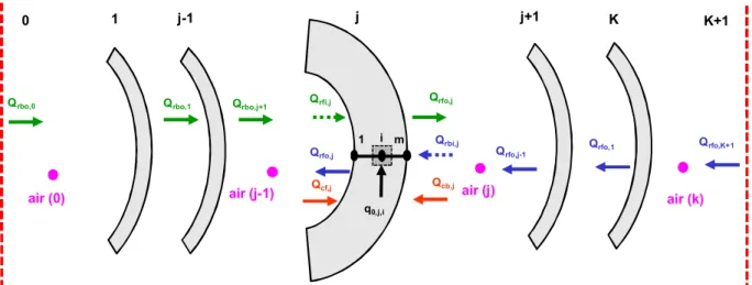
The ceiling diffuser is bounded by the glazing at the pipe exit surface (if any), and the indoor environment. The ceiling diffuser may include multiple (K) domed glazing panes. The panes are numbered in increasing order from the outside to inside environment of the diffuser. Figure 6 shows the convective and radiative heat flows through a multi-pane diffuser.
Figure 6: Radiative and convective heat flows through the ceiling diffuser
Conduction heat transfer
Equations (1), (3), (8), and (12) developed for the collector also apply to the ceiling diffuser, but by inversing the order of the panes and the corresponding heat fluxes. The discretized equations (7), (11) and (14) will read as follows: j K 1 Qrbi,j Qcb,j Qcf,j Qrfo,j q0,j,i Qrfo,j Qrfi,j i Qrbo,1 Qrfo,1 1 m air (j-1) air (j) j+1 j-1 Qrbo,j+1 Qrfo,j-1 0 Qrbo,0 Qrfo,K+1 K+1 air (0) air (k)
− 1 −∆ , . , + ∆ ∆ + 2 , − 1 + ∆ , . , = ∆ ∆ , + ∆ . , , + , , − , , ; i = 2 to m − 1 (98) ∆ ∆ + 2∆ ∙ ℎ , + 2 ∙ 1 + ∆ , ∙ , − 2 ∙ 1 + ∆ , ∙ , = ∆ ∆ , + 2∆ ∙ ℎ, ∙ , + , , + , , − , , ∙ ∆ (99) ∆ ∆ + 2∆ ∙ ℎ, + 2 ∙ 1 − ∆ , ∙ , − 2 ∙ 1 − ∆ , ∙ , = ∆ ∆ , + 2∆ ∙ ℎ , ∙ , + , , + , , − , , ∙ ∆ (100)
The net absorbed solar radiation flux density at the diffuser panes (qsol) in equations (98) to (100) is also given
by equation (2).
Convective heat transfer
The average film coefficient at the front surface (hc,0) of diffuser is equal to that of the pipe exit glazing (hc,N+3)
if it exists, or to that of the pipe floor surface (hfl) if there is no glazing at the pipe exit surface. The film coefficients
of the air spaces between the upside down domed panes of diffuser are obtained from Nu relationships for upright domed cavities by inversing the temperature boundary conditions using relationships similar to equations (94) and (95). If the diffuser panes are flat, correlations for natural flows between concentric disks should be used (Raithby and Hollands, 1998). The film coefficient at the indoor space (hc,K) is usually a fixed input, or calculated for
natural flows over domed or flat surfaces.
Radiation heat transfer
Equations (20) to (23) are used for the radiative heat balance at the glazing panes, with the boundary incident radiation fluxes and pane view factors given by the following relations:
, = , + F ∙ , (101)
, = , ∙ J (102)
, = 1 (103)
, = MIN 1;1; , ∙ , / , ; j = Kj = 1 to K − 1 (104)
Where Jinis the radiosity of the indoor environment (W/m2, Btu/h/ft2).
For a given temperature distribution within a TDD system, equations (20) and (21) with the boundary equations (101) and (102) may be solved using a sequential iterative procedure, in which equation (20) is solved first for all layers (j = 1 to K), followed by equation (21). The process is repeated until convergence is reached. Convergence is declared if the maximum relative change in the layer radiation fluxes is less than a fixed tolerance value.
SOLUTION PROCEDURE
The main unknowns to be solved for a TDD system include the temperature distribution in TDD glazing layers and average temperatures of the enclosed air cavities. The previous analysis showed that the obtained equations for heat flows in TDD systems are non-linear and inter-linked. An iterative procedure must, therefore, be used to obtain the temperatures distributions. The temperatures of air cavities may be deduced from the temperatures of TDD surfaces in contact with the adjacent air spaces using equations (17) and (61). To obtain temperature distribution in TDD glazing layers, there are two possible procedures: direct and sequential. The direct procedure involves a non-linear system of equations whose unknowns are the nodal temperatures of all TDD layers. Suitable technique such as, for example, matrix inversion, may be used to solve for the nodal temperatures simultaneously at each iteration. The sequential procedure involves the simultaneous calculation of the nodal temperature distribution in each TDD glazing layer, by proceeding sequentially to the next layer until covering all TDD glazing layers at each iteration. The direct procedure involves complex formulation to obtain the matrix elements of the system of equations. It may result in fast convergence (low number of iterations), but its calculation time may be a burden as it involves a large porous matrix that needs to be solved at each iteration. The sequential procedure, on the other hand, involves a simple formulation (a tri-diagonal matrix for each TDD pane). It may result in slow convergence (large number of iterations) and some instability issues, but its overall calculation time may be short, depending on the size of a TDD system. Table 1 summarizes the proposed solution algorithm using the sequential procedure.
1. Initialize the nodal and air temperatures of a TDD system; 2. At each iteration (main loop):
3. Compute the convective film coefficients at each TDD surface and air cavities using existing correlations of Nu versus Ra;
4. Compute the air temperatures of TDD enclosed cavities using equations (17) and (61). A tri-diagonal matrix solver may be used for equation (61); Sub-internal iterations should be used to reach a converged solution of equation (61);
5. Compute the radiation fluxes through the collector, entrance glazing, pipe, exit glazing and ceiling diffuser using the recursive system of equations (20) and (21). Sub-internal iterations should be used to solve the system of equations until convergence is reached;
6. Compute the nodal temperatures of each TDD pane, starting from the exterior pane of collector till the last pane of ceiling diffuser. A tri-diagonal matrix solver is used for equations (7), (32), (47), and (98);
7. Evaluate the maximum or cumulative errors in nodal temperatures between two successive iterations; 8. Exit the main iteration loop if the sum of the temperature errors is lower than a tolerance value (fixed input),
otherwise proceed on to the next iteration (step #3);
9. After convergence from the main iteration loop, compute the convective heat fluxes at the front and back sides of each TDD pane using equations (9) and (13), and the net radiative heat fluxes at the front and back sides of each TDD pane (difference between the outgoing and incident fluxes: Qrfo- Qrfi, and Qrbo- Qrbi);
Thermal Characteristic of TDDs
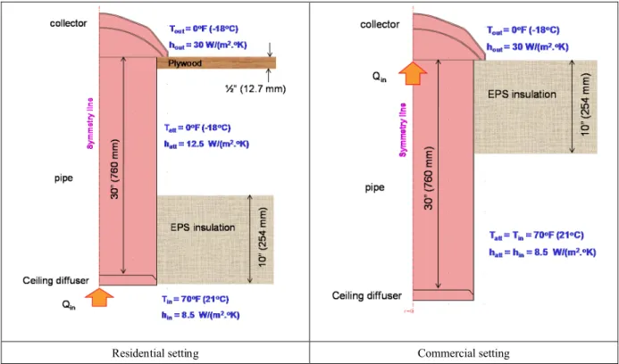
Thermal characteristics of TDDs include the Solar Heat Gain Coefficient (SHGC) and U-factor. The SHGC is defined as the ratio of the total solar radiation flux transmitted indoors to the solar radiation flux incident on the TDD pipe aperture at given sun altitude angle from the vertical and the azimuth angle from the south direction (more details in Laouadi et al. (2013b) on the proposed rating angles). The U-factor is defined as the heat loss from a TDD system to the outside per unit surface area and temperature difference between the inside and outside environments. While the foregoing thermal analysis is for any thermal boundary conditions around any TDD system, the rated thermal characteristics of TDDs are evaluated according to the NFRC 100/200-2010 (NFRC, 2010c,d) rating procedures. The NFRC procedures use standard thermal boundary conditions and model sizes. A TDD system is rated with a vertical straight pipe, placed entirely in the attic space for the residential setting (insulation at ceiling level), or in the plenum space for the commercial setting (insulation at roof level). Figure 7 shows the NFRC standard conditions for the U-factor calculation. It should be noted that hybrid TDDs (TDDs whose pipe has more than one geometry component such as TDDs with circular-to-square adaptors and square ceiling diffusers used in building spaces with suspended or open ceilings) are rated with a portion of the pipe enclosed in a curb space and exposed to the outdoor conditions.
Following the NFRC 100/200-2010 rating procedure (NFRC, 2010c,d), or the ISO standard 15099 (ISO, 2003), the SHGC and U-factor are calculated as follows:
= + ( ) ( )
, (106)
− = ∙|( )| (107)
Where:
Qin : heat loss or gain flux (Figure 7) exchanged between TDD system and indoor environment, evaluated at the
ceiling interface for the residential ratings (insulation at ceiling level), or at the roof level for the commercial rating (insulation at roof level) under the presence (Ibt 0) or absence (Ibt= 0) of solar radiation (W, Btu/h)
Tin : temperature of the indoor environment (C, F)
Tout : temperature of the outdoor environment (C, F)
Residential setting Commercial setting
Figure 7: NFRC standard thermal boundary conditions for U-factor rating of TDDs
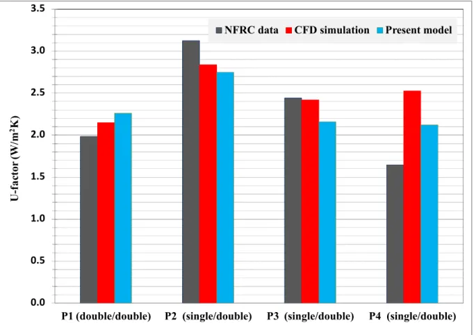
Model Validation
The previous simplified thermal model to compute the thermal performance of TDDs is validated against third party measurement and detailed computational fluid dynamic (CFD) simulations. The measurement data for U-factors were taken from the NFRC certified product directory database (NFRC, 2011), and respective manufacturers supplied the detailed CAD drawings for the CFD simulations. The validation methodology is described below. SIMULATED PRODUCTS
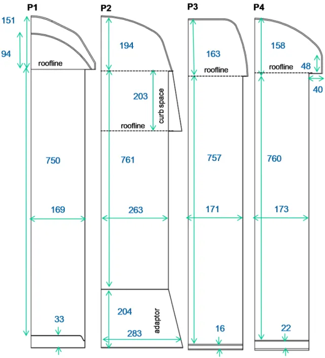
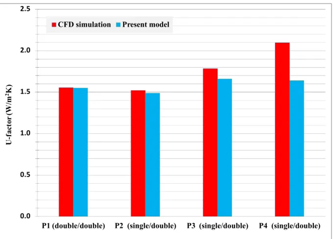
Four commercially available TDD products were selected from the NFRC product database. Table 2 summarizes the physical characteristics of the selected TDDs, and Figure 8 shows their geometrical details. Note that product P2 is a hybrid TDD with a domed ceiling adaptor and square diffuser, and a pipe section (0.203 m, 8”) in a curb space above the roofline exposed to the outdoor conditions. The four TDD products were simulated under the residential rating conditions (Figure 7), and product P1 and P2 with and without an exterior curb section were simulated under the commercial rating conditions.
Table 2 Physical characteristics of the simulated TDDs TDD product Component Descriptions
P1
Collector 3 mm double acrylic glazing
Pipe 0.5 mm Aluminum. The inner surface was coated with a dielectric reflective film with an assumed emissivity of 90%.
Diffuser 1 mm frosted over 0.6 mm prismatic double acrylic glazing
P2
Collector 3 mm single acrylic glazing
Pipe 0.5 mm Aluminum. The inner surface was coated with a dielectric reflective film with an assumed emissivity of 90%.
Diffuser 1 mm over 2 mm double acrylic glazing
P3
Collector 3 mm single acrylic glazing
Pipe 0.5 mm Aluminum with a reflective coating on the inner surface with an assumed emissivity of 3% (ASHRAE, 2009).
Diffuser 3 mm double acrylic glazing
P4 Collector 3 mm single acrylic glazing.
Pipe 0.5 mm Aluminum. The inner surface was coated with an Enhanced Silver film with an assumed emissivity of 2% (ASHRAE, 2009)
Figure 8. Simulated TDD products (dimensions in mm)
CFD SIMULATIONS
The NRC hygrothermal computer program (hygIRC-C) was used in this study. hygIRC-C is a versatile computational fluid dynamic (CFD) program, built under the platform of COMSOL Multiphysics (COMSOL, 2009). The hygIRC-C program simultaneously solves nonlinear multi-dimensional moisture and energy transport equations, long-wave surface-to-surface radiation equations, Navier–Stokes momentum equations in gas cavities,
and Darcy or Brinkman equations in porous layers. hygIRC-C uses the Finite Element Method (FEM) to discretize the governing equations. The program has been extensively benchmarked in previous studies against experimental data (Saber et al., 2010a,b; Saber et al., 2011; Saber et al., 2012a,b,c).
For vertical TDD systems, buoyancy-driven flows in TDD cavities are symmetrical with respect to the TDD axis of revolution (z-axis). A two-dimensional model was thus developed for the CFD analysis (note that a three-dimensional model was also implemented, but produced the same result). The CFD simulations used the following assumptions to solve the various heat transfer modes in a TDD system:
Buoyancy-driven flows in air cavities are incompressible, laminar, and steady-state.
The physical properties of air are constant, except for density in the body force terms in the momentum balance equations. The constant physical properties of air are evaluated at the average temperature of the bounding surfaces.
The fluid density is given by the Boussinesq approximation.
Compression work and the viscous dissipation energy in the energy balance equation are neglected.
The values of thermal properties (conductivity and emissivity) of the TDD materials (aluminum, silver, and acrylic) were taken from the ASHRAE material database (Chapter 33 and Table 5) (ASHRAE, 2009). One exception was that the emissivities of materials with unknown coatings were assumed as shown in Table 2.
Numerical procedure
The numerical approach of the present CFD model used the finite element method. To assure that the numerical results were mesh-independent, a non uniform mesh was selected with finer sizes near the boundaries in order to capture the thermal and momentum boundary layers. Typically, the numerical mesh was refined by doubling the number of nodes until the final results did not appreciably change. Triangular elements were chosen to capture the curved computational domain with less discretizing error. To assure that the steady-state solution was independent on the initial temperature conditions, the numerical simulations were conducted using different initial temperature fields for each TDD product. Two numerical simulations with and without radiation heat transfer were conducted for each TDD product. Radiation heat transfer was turned off by setting the long-wave emissivity of TDD surfaces to zero. More details on the CFD simulation methodology and detailed results for the flow and temperature fields in the selected TDD systems are to be presented in separate studies.