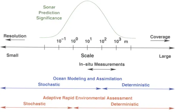
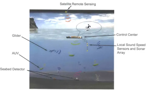
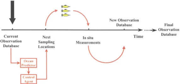
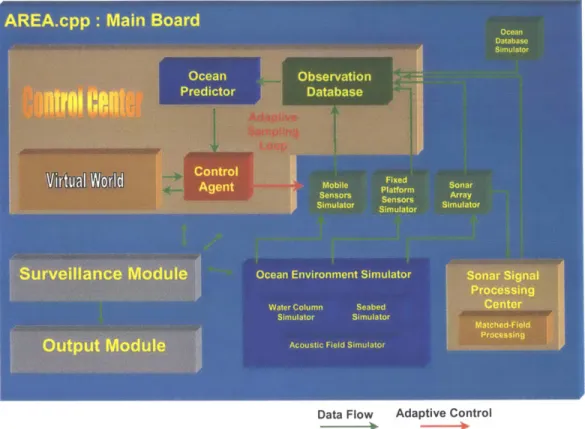
Adaptive rapid environmental assessment system simulation framework

The simultaneous measurement of both heat and ionization signals provides an excellent event by event discrimination between nuclear and electron recoils.. The ratio of the

To support the optimal digitizing system selection according to a given application,the two databasesare coupled with a decision process based on the minimization

The changes of geographical entities in the real world or the changes of data collection standards may result into update operations which modify the content of the database

This paper describes a consistent updating processus over a Geographical Data Base (GDB) as a complex operation concerning Geographic Information Systems (GIS). Our purpose is

The Ecoscore System (ES), based on ecoscores calculated from a battery of liquid and solid phase bioassays, proved to be a robust method which allowed us to evaluate

Thanks to Honduras, Peru, Brazil, Paraguay and Costa Rica, the value of agricultural exports from Latin America and the Caribbean increased by 3.8 percent in August 2020 compared

IICA itself has developed discussion sessions and forums, such as the IICA Blog, where it emphasizes the importance of working jointly on these pillars, especially

The Ministry of Agriculture and Rural Development has advised that agricultural producers who have workers employed to their operations, and whose income from production activity