Analytic Theory of the Gyrotron Lentini, P. J.
Plasma Fusion Center
Massachusetts Institute of Technology Cambridge, MA 02139
by
Philip Joseph Lentini
SUBMITTED TO THE DEPARTMENT OF PHYSICS IN PARTIAL FULFILLMENT OF THE REQUIREMENTS
FOR THE DEGREE OF
BACHELOR OF SCIENCE
at the
MASSACHUSETTS INSTITUTE OF TECHNOLOGY
June 1989Copyright (c) 1989 Massachusetts Institute of Technology. All rights reserved
Signature of Author Department of Physics
June
5,
1989
Certified by0.
Accepted byRichard J. Temkin
Thesis Supervisor
Professor Aron M. Bernstein
Chairman, Undergraduate Thesis Committee
by
Philip Joseph Lentini
Submitted to the Department of Physics on June 5, 1989 in partial fulfillment of the requirements for the degree of Bachelor of Science.
Abstract
An analytic theory is derived for a gyrotron operating in the linear gain regime. The gyrotron is a coherent source of microwave and millimeter wave radiation based on an electron beam emitting at cyclotron resonance fl in a strong, uniform magnetic field. Relativistic equations of motion and first order perturbation theory are used. Results are obtained in both laboratory and normalized variables.
An expression for cavity threshold gain is derived in the linear regime. An analytic expression for the electron phase angle in momentum space shows that the effect of the RF field is to form bunches that are equal to the unperturbed transit phase plus a correction term which varies as the sine of the input phase angle. The expression for the phase angle is plotted and bunching effects in and out of phase (0 and -n) with respect to the RF field are evident for detunings leading to gain and absorption, respectively. For exact resonance, field frequency o= Q, a bunch also forms at a phase of -t/2. This beam yields the same energy exchange with the RF field as an unbunched, (nonrelativistic) beam.
The frequency pulling equation, Awo/o, as a function of detuning, field amplitude, and interaction length is also derived in the linear regime. The linear theory predicts that a gyrotron can be tuned an amount IAo/oITot =-Qf3/
P13
2L, where13±
($11) is the perpendicular (parallel) velocity divided by c, and L is the interaction length.The gain process is shown to depend explicitly on the use of the relativistic equations of motion and the variation of electron mass with beam velocity. These analytic results give a simple explanation for gain in the gyrotron that is useful to those learning about this device. It also provides a relatively simple framework for understanding the physics of the gyrotron in detail without use of numerical techniques. Some of the results derived are believed to be new, and have not been found by other, more rigorous techniques.
Thesis Supervisor: Richard J. Temkin
Dedication
To Rick Temkin, whose excellent support and advice made this thesis possible. To Susan Hakkarainen, who gave me a head start on the math and who has been a good boss and
friend. To Ken Kreischer, who helped me to understand gyrotrons and bunching. To Sam
Chu, whose help with the computer and general good humor made the work a little easier. Most of all to my parents, Salvatore and Grace Lentini, whose sacrifice and support were indispensible to me during my years at MIT.Table of Contents
Abstract 2Dedication
3
Table of Contents
4
List of Figures
5
1. Introduction 62. Physics of the Gyrotron 7
2.1 Brand's Derivation 7
2.2 Normalization of Equations 12
2.2.1 Determination of Parameters 13
3. Electron Bunching 16
3.1 Bunch Angle vs. 8 16
3.2 Inertial vs. Force Bunching 22
4. Frequency Pulling 24
5.
Effect of Relativity
30
List of Figures
Figure 2-1:Figure 2-2:
Figure 3-1: Figure 3-2: Figure 3-3:Figure 3-4:
Figure 4-1:
Figure 4-2:
Figure 4-3:
Figure 4-4:Physical Setup of the Gyrotron W" vs.
8
0 vs. Vi for 8= +2.6, g= 30, F= 0.019, 0.19
0 vs. Vi for 8= 0, g= 30, F= 0.019, 0.19
0 vs. Vi for 8= -2.6, g= 30, F= 0.019,0.19
Initial and Final positions of Eight Electrons; F= 0.19, g=30
Frequency Pulling, Work vs. 8 for 8 negative, p= 30Frequency Pulling, Work vs. 8 for 8 positive, p= 30 Frequency Pulling, Work vs. 8 for 8 negative, p= 1000 Frequency Pulling, Work vs. 8 for 8 positive,
=
10007
15
18
19
20
21
26
27
28
29
Chapter 1
Introduction
The gyrotron, or electron cyclotron resonance maser, is a novel and important microwave and millimeter wave generation device. Gyrotrons are currently being used for Electron Cyclotron Resonance Heating (ECRH) of plasmas in plasma fusion experiments.
The gyrotron basically consists of a resonant cavity in a strong, continuous magnetic field. A beam of relativistic electrons enters the cavity and interacts with the RF (microwave) fields present in the cavity. The gain mechanism consists of a transfer of energy between the electrons and the RF field. The electrons must be moving at relativistic speeds so that their mass will change as their velocity changes. This leads to the formation of bunches of electrons in areas where the electrons lose energy to the RF field.
Most current theories of the gyrotron use particle simulation or some other numerical technique to model the behavior of the electrons and the RF field. Although this method is very useful for designing a gyrotron, it does not offer much insight into the basic physics of the device. This thesis investigates simpler, analytic methods of studying the interaction between the electrons and the RF field. The analytic expressions derived show the bunching effect, and offer deeper insight into the gain mechanism.
This thesis is based upon work done by Brand [2], who derived the basic analytic
expressions of the gyrotron. In his paper, Brand worked out the gain equation, and demonstrated which conditions would lead to a net emission of energy by the electrons. The purpose of this thesis is to extend that work by investigating the electron bunching effect directly, and determining the location of the electron bunches which lead to maximum gain, maximum loss, and other cases. This thesis will also investigate the frequency pulling (Ao/o) of a gyrotron.Chapter 2
Physics of the Gyrotron
2.1 Brand's Derivation
The derivation presented here follows that found in [2]. Figure 2-1 shows a side view
of the idealized gyrotron treated in this thesis. A single beamlet of electrons moving in the
z
direction traverses a cavity in which there is a continuous, uniform magnetic field. Due to
the field, the electrons gyrate in their orbits at the cyclotron frequency:
SeB
(2.1)
yMi
where
BO
is the strength of the magnetic field, mi is the rest mass of the electron, and y is
the relativistic factor:
y=/
-
=-Fl-
(2.2)
22
The cavity also contains the RF field
E=Ele"lm,
which is perpendicular to the field,
and in this case is considered to point in the y direction. For most of the equations derived
here, it is only necessary to use the real part of the field, E=E'
coswe.
The field frequency
(o
is approximately equal to the cyclotron frequency Q. Because this treatment is based
upon a small-signal analysis, the field strength El
is a first order quantity.
When electrons enter the cavity, some are accelerated by the RF field, causing a
relativistic increase in mass, and therefore, a decrease in cyclotron frequency. This causes
these electrons to slip back in their orbits. Other electrons are decelerated by the RF field,
causing a relativistic decrease in mass and a corresponding increase in cyclotron frequency.
These electrons then move ahead in their orbits. The net effect is the formation of a bunch
of electrons at some angle relative to the electric field. The location of this bunch will
determine the sign and magnitude of the energy transfer between the electrons and the RF
field.
The equabion of motion of the electrons is simply that of a charged particle moving in
an electric and a magnetic field:
dp
_e (El cos otj + v xBo k)
(2.3)
dt
The momentum vector p can be separated into the components px, py, and p., with p_ being
the momentum parallel to the magnetic field. It is possible to convert px and py to other
coordinates using the definitions px=-pj sin i and pY=p1 cosw, where pL is themomentum perpendicular to the magnetic field and V is the angular position of the electron
in momentum space. It is then possible to write the equations of motion of the separate
components as:
-- eEcoswtcosN (2.4)
dt
= +
eE
cos siNo
(2.5)dp.
= 0
(2.6)
These equations have zero order solutions of:
P 0 (2.7)
- 4+1 (2.8)
P= A (2.9)
At this point it is convenient to define
0=
ot - x and Q, = CO/y
.0
is the anglebetween the electron and the RF field, and Di is the initial value of the cyclotron frequency.
It is possible to expand equations (2.4) and (2.5) using the identities for products of sines
and cosines. This produces a sum of terms oscillating at frequencies of (o
+f) and
(o
-
92). Because Q,- ~ o the sum of the terms produces a frequency approximately twice
that of Q while the difference of the terms produces a frequency much less than that of 0.
Since we are interested only in changes which occur over many cycles, we may ignore the
rapidly varying part. It is also possible to change from time derivative to spatial derivative
over z, using the identity d/dt
=
v. d/dz. When these substitutions are made, equations (2.4),
(2.5), and (2.6) can be rewritten as:
dp
1eE'
=
-
1cos 0
(2.10)
dO (0
d-
-00
+eE'
sin
(2.11)
dz v,y
v, 2p v. dpz 0 (2.12)To derive p
1to first order in El it is necessary to obtain the zero-order solution of 0.
00 = Bz - N; (2.13)
V.i
P , is found by substituting 00 into equation (2.1O)and integrating. The final answer for p
1is
found to be:
eE'
[
-Cos1
sin-00PIPJ.
2(o-Qj)
I
V
sij
-
si
z
cosO
0(2.14)
2(CO-1,) (vi
Before 0 can be derived, it is necessary to determine y, since this quantity appears in
equation (2.11) when the substitution v,
=
p'/rn, is made. Because y is velocity dependent,
it will change as p
1changes. It is possible to write y in terms of the first order change in
momentum p'
1from equation (2.14):
Y = + Y Pi2P 1 (2.15)
When this is substituted into equation (2.11), 0 to first order in El can be expressed
as:
0=0
zi
eE'sinO F i2 +2-
s.[1 2piu((o-Qj) W-R vi +o -co --eE
cosO
+ Co$2+ co-sos
0-2piL(o-Q)
CO-ngvzi
Using equations (2.14) and (2.16) it is possible to find the work done by the field.
The work done by the RF field on an electron is defined to be:
W=Re [J-e
EI. vdt
(2.17)
When rapid fluctuations of the work are disregarded and the variable of integration is
changed from t to z, this equation can be rewritten:
1 L
W= -- eElp, cos0 dz
(2.18)
To carry out this integration it is necessary to separate the variables pj and 0 into
their zero order and first order parts, and use the identity for the cosine of a sum. Assuming
that 0, is small, it is possible to make the substitution cosO
1=_1 and sin O, =01. W can then
be expressed to second order in El as:
W=
2p
(p1O cos 00 +pj cos 1_L-p0
sin 0) dz
(2.19)This equation for W only applies for an electron of a certain phase. It is therefore
necessary to average W over all phases
jiyfrom 0 to 2n to obtain the ensemble average:
1 2n
<W> -
W dVi
(2.20)
2 n fo
The first term in equation (2.19) represents the work done by the unperturbed
electrons, and goes to zero when averaged over the initial phase. The other two terms are
non-zero and give the final result for the work done:
W
= 2 2
-E
cos L)-14yjm0(W_-Q,)2
L
I_i
( VUi1
2L
,-+ -($P)2 -sin
L)
(2.21)2
v
2i
(
vzi
I
for <W> to be negative for emission to occur. The conditions under which <W> is
negative are examined in the next section.2.2 Normalization of Equations
At this point it is convenient to rewrite equations (2.14), (2.16), and (2.21) in terms of three dimensionless parameters, in order to normalize the equations and make them clearer. The dimensionless parameters are defined as:
8= -L (2.22) V. F=ek - (2.23) p -Li V. S2 =
L
(2.24)
V.iThe parameter 8 represents the net detuning between the frequency of the RF field and the cyclotron frequency after the electrons have left the cavity; F represents the normalized EM field strength; and R represents the dimensionless relativistic interaction time or length. Before the equations can be rewritten in terms of these parameters, it is necessary to redefine equations (2.14) and (2.21) as dimensionless quantities. This is done by dividing the quantities by some convenient expression with the proper units:
p? =-
(2.25)
p.
112
W,=<W>
I
(2.26)2y
m
Now equations (2.14), (2.16), and (2.21) can be rewritten in their dimensionless, parameterized form. These equations are functions of L and not of z, indicating they represent final values after the electrons have left the cavity.
p,= I -F
[sin
iyj + sin(8 - y)] (2.27)0=
-+
[-gsinyV +[1-g]
-
[cos1v-cos(S-w,)]
(2.28)
Wfl
=
1- cos (8)
+
+cos()-
(2.29)
2.2.1 Determination of Parameters
F, as defined in equation (2.23), can be shown to be:
F=
eEIL
(2.30)
The order of magnitude of the RF field, E, can be found using the equation
Power
1 E
2(2.31)
2zo
where
zo
is the free space impedance, 377 ohms. Using $
=0.4, $
=0.2, and L
=
1 cm,
and letting the power range from 1 kW to 100 kW, F is found to vary from 0.02 to 0.2.
In order to find R, equation (2.24) is changed to:
2
$i +
(2.32)
Using the same parameters used to calculate F, and additionally assuming that L/A=5,
la is found to be approximately 30.
8 can take on any value, however, there are three main cases of interest. Figure 2-2
shows a plot of W, for the cases g= 0, 10, 30, and F= 0.19. It is not necessary to make
additional plots for other values of F, as F is a scaling factor which would only change the
height of the curve, and would not affect its dependence on S. The R= 0 plot is never less
than zero, indicating that the electrons must be moving at relativistic speeds to obtain gain,
as g is dependent on Pi. The curve for g= 30 has a minimum at 8=+2.6 and a maximum at
8=
-2.6. Maximum gain occurs at 8= +2.6, which demonstrates that the RF field frequency
co must be greater than the cyclotron frequency Q2 for gain to occur. It is also interesting
that all three curves intersect at 8= 0, indicating that in the limit as 8 goes to zero, W,
becomes independent of g.
-15-Figure 2-2: W, vs.
S
-60
40 w 20 0 r 3 0 t -t
--5 0 De I 5 , *, ' -20 -A -10=0
= 10
10Chapter 3
Electron Bunching
3.1 Bunch Angle vs. 5
The location of the electron bunch depends upon the value of 8, according to equation (2.28). This equation consists of four terms. The first two terms represent the unperturbed angle which is a result of the natural progression of 0 as the electrons travel through the cavity. These terms, when plotted on a 0 vs. Ni plot would produce a straight line. The last two terms represent the effect of the RF field upon the electrons. 0 can be defined as:
0F= + R (3.1)
where
R=(-g-sin8+asin5 sinw, + (1-cos8-1 +cos) cosvi (3.2)
Using the identity: A sinx + Bcosx =
A + B 2 sin tan- + ) sin (x + tan' (3.3)
it is evident that
S=
s
-v
+ [(A+B/2
sin (tan- I+ it sin Vw+tan-IB) (3.4)where
A = - -sins +I sin 8 (3.5)
B
=1-cos6-LL+cos8
(3.6)
For a fixed value of the detuning 6, the evolution of the angle 0 as as a function of the input phase angle y is seen to be:
S= 8 - Vi +f,
(8) sin (xVg
+ (8)) (3.7)where
fj()F
I
.
B
t
(3.8)
f ( 5)= A + B 2 sin tan- +(.
$A tan- (3.9)
This shows that the angle 0 is described by a single sinusoidal bunching effect added to the unperturbed case.
Figures 3-1, 3-2, and 3-3 show 0 vs. xy for the case R= 30, F= 0.019 and F= 0.19. The F= 0.019 plot is close to the unperturbed case and shows a near uniform distribution of 0 over x,. The F= 0.19 plot, however, shows a plateau forming at a certain angle 0, indicating that electrons starting over a certain range of y finish over a much narrower range of 0. This implies that these electrons are being pushed together in a bunch. The approximate location of these bunches is 0= 0 for 8= +2.6, 0= -n/2 for 8= 0, and 0= -n for
5= -2.6.
The location of the bunch corresponds to the work done in each of the three cases. 0~ 0 means that the electron bunch is moving in the same direction as the RF field when it leaves the cavity. Since an electron has a negative charge, the electrons in the bunch will be decelerated by the field, transferring energy to the field. O~ -7t means that the bunch is moving directly against the RF field. These electrons will be accelerated, causing a loss of energy by the RF field. 02 -n/2 means that the bunch is moving perpendicular to the RF
Figure 3-1: 0
vs. Ay
for
S=
+2.6, p= 30,
F=
0.019,0.19
3 2 1 0 T h e --2 -3 -4 -5 0 3 4 Initial Psi 5 F=0.019---F=0. 19
2 I II
I ~ I~ ~ I II
I
I
p 6 7 IFigure 3-2:
0
vs. yi for
=0, ,=
30, F= 0.019, 0.19
2 3 4 5 In i t i a I Ps iF= 0.019
-F= 0. 19
0 T h e -4 t I ~I
I jI
I
-6 -8 0 6 7 -2i
1Figure 3-3: 0 vs. N'~for 8= -2.6,
j=30, F= 0.019,0.19
2 3 4 In it ialI Psi 5F= 0.019
-F=0. 19
-4 Te
a
-6 I I-' -8F
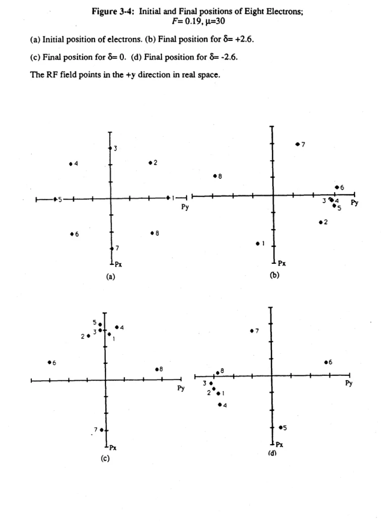
-0 6 7 1Figure 3-4: Initial and Final positions of Eight Electrons;
F= 0.19, I±=30
(a) Initial position of electrons. (b) Final position for 8= +2.6.
(c) Final position for 8= 0. (d) Final position for 8= -2.6.
The RF field points in the +y direction in real space.
.4 '3 .2 Py *1 9-.7 +6 65 Px (b) Px (a) .7 .8 3.0 Py 2 0. 04 *6 Py Px (d) 20 3* I I 7 04. .LPx (C) I
field as it leaves the cavity, implying little or no interaction between the electrons in the bunch and the RF field. In this case W, is zero only because of the effect of the non-bunched electrons.
Another method of examining the bunching effect is to take an ensemble of electrons with the same p1 and uniformly distributed in phase, and find their final p1 and xV in the three cases. This is shown for eight electrons in figure 3-4. The axes are p, vs. -p". These plots were done for the same parameters as the previous plots: F= 0.19, R= 30, 8= +2.6, 0, -2.6. Again, it is apparent that the location of the bunch explains the value of W, in each case. For 8= +2.6, the bunch forms where p, is at its maximum positive value, indicating that the electrons are moving in the same direction as the RF field. For 8= -2.6, the bunch forms where p, is at its maximum negative value, showing that these electrons are moving directly against the RF field. For 8= 0, the bunch forms where p, has its maximum negative value, indicating that these electrons are moving perpendicular to the field. When the electrons leave the region of the RF field, they continue to gyrate in circles about the magnetic field B0. Particles which move around a circle have a position vector perpendicular to their momentum vector. Because of this, an electron which has a momentum of p, = p_, px = 0 must be at the position (x,0). Therefore, the axes in figure
3-4 could be relabeled to x vs. y, demonstrating that bunching occurs in real space as well as momentum space.
3.2 Inertial vs. Force Bunching
Two simultaneous processes occur which lead to bunching. Inertial bunching occurs
when the field acts upon p
1, changing y and hence also changing the cyclotron frequency by
equation (2.1). This causes the electrons to slip either ahead or back in their orbits to form the bunch. Force bunching occurs when the field directly moves the electrons in their orbits to form a bunch. Inertial bunching is introduced into equation (2.16) by the p term fromequation (2.15). Equation (2.16) is then separable into separate equations, representing the
inertial and force bunching:
i=
[-F
- sin 4fv -[Cos
-Cos( -4f)] (3.10)F
fo =
[cosy-cos(8-Xy)]
(3.11)
Tot = (5 - Vi)+ (in + (3.12)
It is also possible to separate
W,into inertial and force terms, in order to compare the
relative strength of the two effects. Using equation (2.19) it is apparent that the second
term represents inertial bunching, since it explicitly contains p . The third term however,
depends upon 0,, which contains both inertial and force bunching terms. The total work is
separable into:
F2
1
_ cos (8) + sin(8) + cos(S)1
(3.13)
"
22
2
\
2
8
0 1
W =
-Cos([) (3.14)Assuming that R >> 1, the first two terms of (3.13) can be ignored. Using this
assumption, W,, becomes proportional to F
2R, while WfO is proportional to F
2. Since F is
proportional to L, and g is also proportional to L, Wi,, is proportional to L
3while Wg is
proportional to L
2. It is evident that Wf
0cannot become negative; it is the product of
squares of terms and a (1-cos5) term. This implies that in the linear theory, the force
bunching cannot lead to gain, however, the results might be different for nonlinear theory.
For the 8= +2.6, R= 30 case, W,
=
-13.7- W.
In this case, the inertial bunching is
the greater effect. For the 8= -2.6 case, W,
=+15.7 -Wf,. Here, the inertial bunching is
even greater. For the 8= 0 case, the two effects are exactly equal.
Chapter 4
Frequency Pulling
The frequency pulling of a gyrotron is A/o. Before an explicit expression can be found for the pulling, it is necessary to solve for D, the imaginary counterpart of W:
D = Im [ -e El - dt (4.1)
Following the same method used to obtain Wn, D is averaged over the initial phase, made dimensionless, and normalized to obtain:
D,=
L
[ n)sin()+-in()( + cos(S)) (4.2)It is now possible to find the frequency pulling, since Ao/o is defined defined by Slater [6] to be:
A
1
D4.3)0
2Q
WnQ
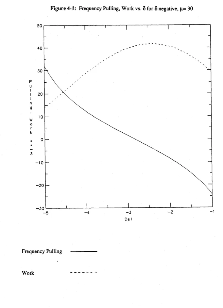
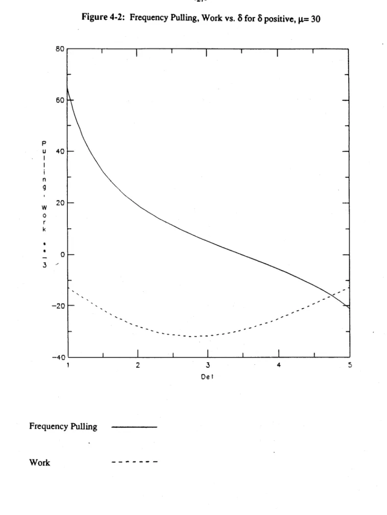
is the quality factor of the gyrotron and is only a scaling factor of the frequency pulling. The pulling and the work done are shown in figures 4-1 and 4-2 for the case F= 0.19, R= 30, andQ=
25. This value ofQ
was chosen so that the variations of Wn and the pulling could be seen on the same scale. There are two separate plots for8 negative and 8
positive because the frequency pulling has a singularity near 6=0. It is apparent from these plots that the frequency pulling is very nearly linear in the regions about 8 = ± n. Making the assumption that g>> 1, it is possible to simplify Adoio in these regions to:Ao
=.
82
(4.4)
0)
-4Qg
This approximation should be valid over the regions -4
<
8 < -1 and 1 < 8 < 4. Over
each of these regions, 8 will vary from 1 to 16. Assuming that the detuning8
does range from 1 to 4, which is the region in which gain occurs, the total range of frequency tuning is:Amo
4
-- jTot =
(4.5)
For a given gyrotron operating at 140 GHz, with a cavity whose
Q is 500, and where
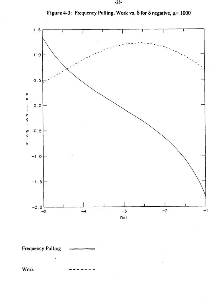
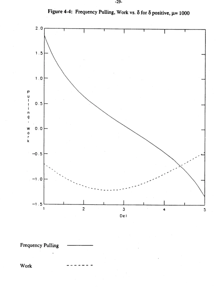
20, Aoorot/o will be approximately 0.0004, and the total tuning range predicted by linear theory will be about 50 MHz. This is reasonably close to the tuning range predicted by nonlinear theory [4], which is approximately 100 MHz.Figures 4-3 and 4-4 show frequency pulling and work for F= 0.019, R= 1000, and
Q=
0.5. Again, the value of
Q
has been chosen so that the curves vary over the same scale. Linear regions still exist about 8= ±in. Because the pulling is proportional to 1/, in this case the frequency cannot be tuned nearly as much as in the R= 30 case.50 40 30 20 10 0 -10 -20
Figure 4-1: Frequency Pulling, Work vs. 6 for 8 negative, p= 30
- --5 -4 -3 De I -2 Frequency Pulling Work P U n w 0 r k 3 -1
Figure 4-2: Frequency Pulling, Work vs. 8 for S positive, g= 30
80 60 40 20 0 -20 -40 2 3 Del 4 Frequency PullingWork
P U n w 0 r k * *. 3 II
I
I
5 1Figure
4-3: Frequency Pulling, Work vs. 8 for 8 negative, g= 1000
1 .5 100 P U n 9 w -0.5 -0 r k -1 .0 -1 .5 -2.0 -5 -4 -3 -2 -1 De IFrequency Pulling
Work1.0t 0.5F 0.0k -1 .0 -1 .5 2.0 1 .5 2 3 De I 4 Frequency Pulling
Work
Figure
4-4: Frequency Pulling, Work vs. 8 for 8 positive, = 1000
-p U n w 0 r k -0.5 5 I
Chapter 5
Effect of Relativity
The change in mass due to relativity is essential to the operation of the gyrotron. This can be seen by investigating what occurs when relativity is assumed to be nonexistent. An absence of relativity means that y = 1, and therefore the mass of the electron is always
equal to the rest mass nmg. The way to accomplish this transformation is to set the second term of equation (2.15) to zero. The previously derived equations can be simply converted to a non-relativistic forn by noticing that g, as defined in equation (2.24), is dependent on Pi. The only term which introduces
Pi
into the equations is the second term of equation (2.15), which has been set to zero. Therefore, it is only necessary to set R to zero in the equations to investigate the effect of relativity.The momentum, pn, does not change with a lack of relativity, since it is not dependent upon a relativistic change in mass. Both 0 and W, however, change dramatically without relativity:
= - + F cos (XV) - cos (8- ) (nonrelativistic) (5.1)
W,,f [1 -cos() (nonrelativistic) (5.2)
2 82
One immediate observation is that W, is now a positive quantity; it is the product of the squares of terms and a (1-cos8) term, and cannot become negative. This implies that it is now impossible to obtain any gain from the device. Another result is that the applied RF field no longer contributes to inertial bunching, since the field term in equation (3.10) is dependent upon [t. The dependence of W. upon the length of the cavity is also dependent upon relativity. In the relativistic case, as R becomes large, W,, goes as F2 g. Both F and R
are directly proportional to L, so the work done is proportional to L
3. In the non-relativistic
Chapter 6
Discussion and Conclusions
Analytic expressions were derived for the transverse momentum and phase angle of electrons in a gyrotron. Expressions were also found for the work done by the field on the electrons, and the frequency pulling of the gyrotron.
The nature of the bunching which occurs in a gyrotron was investigated. It was found that bunching occurs in a sinusoidal manner. It was also seen that the location of the bunch is dependent upon the detuning factor 8, and the size of the bunch, that is, the proportion of electrons which go into the bunch, is dependent upon the strength of the RF field. The location of the electron bunch was found for three separate cases: maximum emission, maximum absorption, and zero detuning. It was found that a bunch forms at 0= -ir/2 for the zero detuning case, a previously unknown result.
The expression derived for the frequency pulling Aoaw is a new result. It was found that the range of frequency tuning is proportional to the square of the detuning
8,
and is inversely proportional to the relativistic interaction length g.References
[1]
Baird, J. Mark.
Gyrotron Theory.High-Power Microwave Sources.
Artech House, Inc, 1987, Chapter 4. [2] Brand, G. F.
Gyrotron or electron cyclotron resonance maser: An introduction.
American Journal of Physics 50(3), March, 1982.
[3]
Kreischer, K. E. and Temkin, R. J.
High-Frequency Gyrotrons and Their Application to Tokamak Plasma Heating.
Infrared and Millimeter Waves 7, 1983.
[4] Kreischer, K. E., Danly, B. G., Woskoboinikow, P.,\Mulligan, W. J., and Temkin, R. J.
Frequency Pulling and Bandwidth Measurements of a 140 GHz Pulsed Gyrotron.
International Journal of Electronics 57(6), 1982.
[5] Robinson, L. C.
Cyclotron Resonance with Free Electrons and Carriers in Solids.
Methods of Experimental Physics. Volume 1O.Physical Principles of Far-Infrared Radiation.
Academic Press, 1973, Chapter 5. [6] Slater, C.
Microwave Electronics.