https://doi.org/10.5194/nhess-17-1837-2017 © Author(s) 2017. This work is distributed under the Creative Commons Attribution 3.0 License.
Assessment of evolution and risks of glacier lake outbursts in the
Djungarskiy Alatau, Central Asia, using Landsat imagery and
glacier bed topography modelling
Vassiliy Kapitsa1, Maria Shahgedanova2, Horst Machguth3,4, Igor Severskiy1, and Akhmetkal Medeu1
1Institute of Geography, Almaty, 050010, Kazakhstan
2Department of Geography and Environmental Science, University of Reading, Reading, RG6 6AB, UK 3Department of Geography, University of Zurich, Zurich, 8057, Switzerland
4Department of Geosciences, University of Fribourg, Fribourg, 1700, Switzerland
Correspondence to:Maria Shahgedanova ([email protected]) and Vassiliy Kapitsa ([email protected]) Received: 5 April 2017 – Discussion started: 29 May 2017
Revised: 11 September 2017 – Accepted: 16 October 2017 – Published: 24 October 2017
Abstract. Changes in the abundance and area of mountain lakes in the Djungarskiy (Jetysu) Alatau between 2002 and 2014 were investigated using Landsat imagery. The number of lakes increased by 6.2 % from 599 to 636 with a growth rate of 0.51 % a−1. The combined areas were 16.26 ± 0.85 to 17.35 ± 0.92 km2respectively and the overall change was within the uncertainty of measurements. Fifty lakes, whose potential outburst can damage existing infrastructure, were identified. The glacier bed topography version 2 (GlabTop2) model was applied to simulate ice thickness and subglacial topography using glacier outlines for 2000 and SRTM DEM (Shuttle Radar Topography Mission digital elevation model) as input data achieving realistic patterns of ice thickness. A total of 513 overdeepenings in the modelled glacier beds, presenting potential sites for the development of lakes, were identified with a combined area of 14.7 km2. Morphomet-ric parameters of the modelled overdeepenings were close to those of the existing lakes. A comparison of locations of the overdeepenings and newly formed lakes in the areas glacierized in 2000–2014 showed that 67 % of the lakes de-veloped at the sites of the overdeepenings. The rates of in-crease in areas of new lakes correlated with areas of modelled overdeepenings. Locations where hazardous lakes may de-velop in the future were identified. The GlabTop2 approach is shown to be a useful tool in hazard management providing data on the potential evolution of future lakes.
1 Introduction
The retreat of mountain glaciers has been observed since the end of the Little Ice Age (LIA) worldwide and has intensified during the last 30–50 years. The mountains of Asia, includ-ing the Pamir, Tien Shan and Djungarskiy (Jetysu) Alatau, where currently glaciers occupy about 16 427 km2 (Sorg et al., 2012), are no exception. Across this region, glaciers re-treated, losing both area and mass (Solomina et al., 2004; Shahgedanova et al., 2010; Kutuzov and Shahgedanova, 2009; Sorg et al., 2012; Yao et al., 2012; Farinotti et al., 2015; Pieczonka and Bolch, 2015), with the highest retreat rates reaching 1 % a−1 reported for the northern Tien Shan and Djungarskiy Alatau (Narama et al., 2010a; Severskiy et al., 2016).
One of the main impacts of glacier recession is an increase in number, area, and volume of glacial and proglacial lakes. These lakes are potentially dangerous as rapid snow and glacier melt can result in lake outbursts threatening life and infrastructure (Richardson and Reynolds, 2000). Many stud-ies of glacial and proglacial lake evolution were published for Asia, focusing on the following three topics: (i) lake in-ventories documenting spatial and temporal trends in lake formation and development, (ii) identification of potentially hazardous lakes and assessment of likelihood of glacial lake outburst flood (GLOF), and more recently (iii) attempts to predict the formation of lakes following de-glaciation.
To date, these studies were mostly concerned with the Hindu-Kush–Himalaya region and the Tibetan Plateau (e.g.
Bolch et al., 2008; Komori, 2008; Ye et al., 2009; Huang et al., 2011; Gardelle et al., 2011; Wang et al., 2012; Zhang et al., 2011; 2013; Fujita et al., 2013). Most reported an increase in number of lakes, their areas and water storage (e.g. Wang et al., 2012). Many studies highlight important regional dif-ferences in lake evolution (e.g. Gardelle et al., 2011; Zhang et al., 2013) showing that trends in changes in lake areas and volumes correlate well with changes in glacier mass bal-ance and other factors such as changes in evaporation, wa-ter withdrawal for human use in the wawa-ter-deficient regions and lake drainage (either deliberate or natural). Possible fu-ture development of lakes in the Karakorum–Himalaya re-gion was investigated by Linsbauer et al. (2012, 2016), who applied the glacier bed topography (GlabTop) model to iden-tify overdeepenings in the glacier beds in which potential lakes may evolve in the future.
Glacial and proglacial lakes in the mountains of Central Asia received less attention. Recently, an inventory of lakes with individual areas in excess of 2000 m2 was compiled by Wang et al. (2013) for the Tien Shan, reporting an in-crease in the count and combined area of lakes of 22.5 % and 16.7 ± 2.9 % respectively between 1990 and 2010. Wang et al. (2015) assessed water storage in lakes of the Tarim Basin, reporting a decline in the levels of glacier-fed lakes, despite the observed glacier thinning and negative mass balance, and they attributed this discrepancy to water abstraction for agri-cultural needs. Bolch et al. (2011) and Petrov et al. (2017) as-sessed hazard potential of 132 lakes in the Zailiiskiy Alatau and of 242 lakes in Uzbekistan respectively. Other studies, including Narama et al. (2010b), Jansky et al. (2010), Medeu et al. (2013) and Herget et al. (2013), and earlier studies from the 1970s to the 1990s reviewed by Medeuov et al. (1993) and more recently by Evans and Delaney (2015) focused on hazard potential of individual lakes, particularly in the densely populated Zailiiskiy Alatau.
The Djungarskiy Alatau is one of the mountain regions of Central Asia where lakes are particularly widespread and where glacier retreat rates are among the highest in the re-gion (Severskiy et al., 2016). Between 1955 and 2011, 48 % of the glacier area was lost; between 2000 and 2011, glaciers lost 12 % of their combined area (Table S1 in the Supple-ment), retreating at a rate of 1.1 % a−1. Vilesov et al. (2013) reported a widespread degradation of permafrost and melt of buried ice across the region. Lake dams are predomi-nantly composed of morainic material, and thawing of per-mafrost and buried ice increases the risk of moraine failure and lake outburst (Popov, 1986; Jansky et al., 2010; Bolch et al., 2011). A number of GLOF events, followed by mud-flows, were reported in the region in the 1970s and early 1980s, when positive temperature anomalies were close to those observed in the 2010s, e.g. in the upper reaches of the Aksu River in 1970 and 1978 and the Sarkand valley in 1982 (Medeuov et al., 1993). In 1982, the outburst of Lake Akkol in the upper reaches of the Sarkand River at about 3200 m a.s.l. and its discharge into Lake Tranzitnoe
and then Lake Kokkol, which were overtopped, led to the formation of the largest recorded mudflow in the region, with an estimated volume of water and transported material of ap-proximately 2.7 million m3. The maximum discharge was es-timated as 2300 m3s−1. Within the town of Sarkand, located 45 km downstream, discharge reached 300 m3s−1, leading to a widespread destruction of infrastructure (Tikhomirov and Shevyrtalov, 1985).
However, despite the rapid retreat of glaciers, abundance of lakes, and recently initiated development projects and ex-panding infrastructure, there is no comprehensive inventory of lakes in the region enabling assessment of their evolu-tion and hazard potential. An inventory for a single year of 2002 was compiled using Landsat imagery by Severskiy et al. (2013) for selected regions in the Djungarskiy Alatau reporting that the majority of lakes were located between 3300 and 3600 m a.s.l. on either young (20th or 21st century) or LIA and older moraines. Medeu et al. (2013) examined changes in 48 lakes in the catchment of the river Khorgos between 1978 and 2011 using the USSR 1 : 100 000 topo-graphic maps and Landsat imagery. This study concluded that the number and combined area of lakes positioned on the 20th to 21st century moraines in proximity to glaciers exhibited the largest change, while those positioned on the older moraines changed the least. The study stressed that opposite trends in lake evolution can be observed within the same relatively small region, particularly with regard to lakes positioned on the young moraines. Kokarev and Shes-terova (2014) assessed changes in glacier area in the southern Djungarskiy Alatau, where they identified 190 lakes with the total area of 6 km2as in 2000 but did not provide any analysis of lake distribution and evolution.
The aim of this paper is to provide a comprehensive inven-tory of lakes and their observed and future evolution in the Djungarskiy Alatau and an assessment of their hazard poten-tial using remote sensing and the GlabTop version 2 model. The specific objectives are to (i) present inventories of lakes for 2002 and 2014; (ii) assess changes in number and area of lakes between these years for different river basins and ele-vation, types and size classes; (iii) assess hazard potential of lakes, providing recommendations for further investigation using higher-resolution satellite imagery and field studies; and (iv) model glacier bed topography and identify overdeep-ened areas where future lakes may develop, testing the results against the observed development of lakes.
2 Study area
The Djungarskiy Alatau is located at the north-eastern flank of the Tien Shan (Fig. 1). The maximum elevation is 4622 m but most peaks extend to about 3800 m. The glacier snouts descend to approximately 3400 m a.s.l. In 1956, the com-bined glacierized area was 814 km2, declining to 465 km2in 2011 (Vilesov et al., 2013). By 2011, 103 glaciers (half of
Figure 1. Study area. GLOF symbols show lakes identified as potentially in danger of outburst. Meteorological stations: 1 – Sarkand (764 m a.s.l); 2 – Lepsy (1012 m a.s.l.); 3 – Jarkent (643 m a.s.l.).
those catalogued in 1956) had disappeared. At present, the northern sector (basins of the Bien, Aksu and Lepsy rivers) is most heavily glacierized, followed by the southern (basins of the Khorgos and Usek) and then western (the Karatal basin) sectors. The number and combined area of glaciers decline towards the east (basins of the Tentek, Tastau and Rgaity) (Fig. 1; Table S1).
The climate is characterized by strong seasonal contrasts in temperature and precipitation (Fig. 2). In winter, the re-gion is dominated by the western extension of the Siberian anticyclone which predetermines low temperatures and small amounts of precipitation. The westerly flow dominates in au-tumn and spring, with frequent depressions and precipita-tion maxima in October–November and April–May. In sum-mer, the thermal Asiatic depression dominates and the ad-vection of warm, dry air from the south results in low precip-itation. Precipitation declines towards the east from 1400 to 1600 mm at the altitude of 3400–3600 m a.s.l. in the west to about 1000 mm in the east (Vilesov et al., 2013). The accu-mulation period extends between mid-September and early June; the ablation period is limited to June–July–August (JJA). 0 20 40 60 80 100 -20 -15 -10 -5 0 5 10 15 20
Jan Feb Mar Ap
r
May Jun Jul Au
g
Se
p
Oct Nov Dec
mm
oC
Precipitation Temperature
Figure 2. Temperature and precipitation climatology for the Lepsy meteorological station (45.32◦N, 80.37◦E; 1012 m a.s.l.), 1960– 2014. Location of the station is shown in Fig. 1.
3 Data and methods
3.1 Satellite and ground-based data
To map glacier lakes, six (nearly) cloud-free Landsat scenes for 2002 and 2014 were obtained from the US Geologi-cal Survey (USGS; http://glovis.usgs.gov/) in the Universal Transverse Mercator (UTM) zone 44 WGS 84 projection
Table 1. Characteristics of the Landsat images used in this study. The July 2014 scene covered an area containing 15 lakes (2 % of all lakes as in 2014).
Satellite/sensor Channels (µm) Path/row Scene ID number Acquisition date Landsat 7 ETM+ 2 (0.519–0.601); 4 (0.772–0.898); 7 (2.064–2.345); 8 (0.515–0.8986) 148/29 LE71480292002237SGS00 25 August 2002 147/29 LE71470292002230SGS00 18 August 2002 147/28 LE71470282002214SGS00 2 August 2002 Landsat 8 OLI 3 (0.525–0.600); 5 (0.845–0.885); 7 (2.100–2.300); 8 (0.500–0.680) 148/29 LC81480292014214LGN00 2 August 2014 147/29 LC81470292014223LGN00 11 August 2014 147/28 LC81470292014191LGN00 10 July 2014
Figure 3. An example of the upper section of a cascade (vertical sequence) of lakes in the Aksu River basin (an oblique aerial photo-graph by M. Kasenov; July 2014). Figure 9a shows a Landsat scene depicting the cascade.
(Table 1). Five out of six scenes were obtained in August to minimize uncertainty associated with seasonal fluctuations of lake levels. According to the data from the Lepsy mete-orological station located at 1012 m a.s.l. (Fig. 1), the JJA temperatures in 2002 and 2014 were very close at 16.9 and 17.3◦C respectively, ensuring similar melt conditions. The selection of the July–August scenes helped to eliminate one of the main sources of uncertainty in lake mapping – the presence of seasonally frozen water and seasonal snow on the frozen surfaces of lakes. It also ensured that lake levels were at their maximum, aiding mapping of the ice contact lakes and lakes located on the young moraines whose areas may be significantly reduced during the cold season. A col-lection of the ground-based and oblique aerial photographs (e.g. Figs. 3, 4) obtained in 2014 was used as supplementary data.
The void-filled SRTM3 GDEM (https://lta.cr.usgs.gov/ SRTM1Arc) and ASTER GDEM2 (https://asterweb.jpl.nasa. gov/gdem.asp) with 30 m resolution were used to derive data on slope angles. SRTM3 DEM (digital elevation model) was used to derive elevations of the lakes. A reliable global DEM
(GDEM) of the study area is essential for the assessment of thresholds for mass movements in the vicinity of lakes and potential debris flow pathways. Both GDEMs were shown to be suitable for assessments of slope angles and elevations in the Zailiiyskiy Alatau with limitations regarding smaller features (e.g. lateral moraines, deep gorges) and steep slopes (Bolch et al., 2011). To assess accuracy of both GDEMs in the study region, elevations of eight ground control points (GCPs) obtained using differential GPS (DGPS) in the ice-free areas were compared with elevations derived from the GDEM. The RMSE values were ±10 and ±15 m for SRTM3 and ASTER2 respectively. However, the number of ground-based measurements is insufficient to quantify uncertainty of slope estimation. Therefore, a comparison between slope an-gles derived from ASTER and SRTM was used to charac-terise uncertainty.
3.2 Lake identification
A total of 599 and 636 lakes were mapped on the 2002 and 2014 images respectively using ERDAS Imagine. All lakes had a natural regime and were not lowered artificially or used for water abstraction. A number of previous studies devel-oped (Huggel et al., 2002; Li and Sheng, 2012) and applied (Ye et al., 2009; Bolch et al., 2011; Gardelle et al., 2011; Wang et al., 2012, 2013) an automated technique for the mapping of lakes using the normalized difference water in-dex (NDWI) based on the low water reflectance in the NIR band and using various band combinations (e.g. green, blue). The well-known advantages of automated mapping are (i) the reproducibility of results and (ii) the ability of the method to quickly map large numbers of lakes. The disadvantages are (i) the inability to map small lakes imposed by the res-olution of multispectral Landsat imagery; (ii) the misclassi-fication of lakes due to shadows (although this problem can be negated by the use of a shadow mask generated using a precise DEM, Huggel et al., 2002); and (iii) a wide range of NDWI values characterising lake pixels resulting from the widely different physical and chemical properties of moun-tain lakes and, consequently, a wide range of their spectral
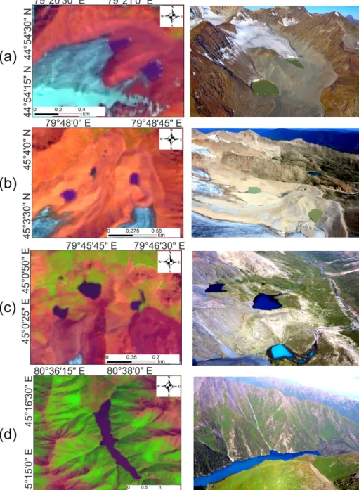
Figure 4. Examples of lakes of different types: Landsat imagery (2014) and oblique aerial photographs (V. Kapitsa; M. Kasenov; July 2014): (a) Type 1 (contact lakes); (b) Type 2 (proglacial lakes on 20th to 21st century moraines); (c) Type 3 (proglacial lakes on LIA and older moraines); (d) Type 4 (rock-dammed lake).
signatures making application of a single threshold to map-ping of mountain lakes problematic (Li and Sheng, 2012). Lakes with high water turbidity are especially difficult to map using automated techniques (Bolch et al., 2011) as are small lakes which tend to have low NDWI values (Li and Sheng, 2012).
In this study, automated mapping of lakes was initially per-formed using various band combinations but did not produce satisfactory results because the method frequently misclassi-fied melting glaciers as lakes and, importantly, consistently
failed to distinguish lakes with high water turbidity, which is particularly typical of the lakes developing on newly formed moraines (Type 2 lakes as defined in Sect. 3.4; Fig. 3). In 2014, there were 234 Type 2 lakes in the study area (37 % of all lakes) and the high proportion of misclassified lakes of this type alone significantly reduced the advantages of the au-tomated mapping with regard to efficiency and reproducibil-ity of the results.
Moreover, small lakes cannot be mapped using automated techniques. Applying NDWI to the Landsat imagery with
30 m resolution, Wang et al. (2013) used a threshold of 2000 m2 in digitization of lake areas as it covered approxi-mately three pixels of uninterrupted water body. In the Djun-garskiy Alatau, 7 % of all lakes had individual areas less than 2000 m2 (Sects. 4, 5). The identification and mapping of smaller lakes was important because, in the study area, they frequently form vertical sequences or cascades whereby several lakes either have a hydraulic connection or are lo-cated in close proximity at different elevations (e.g. Fig. 3). While an outburst of a single small lake is unlikely to cause severe damage, it can trigger an outburst of a larger or mul-tiple lakes. Having reviewed a number of studies document-ing debris flows in the northern Tien Shan, Evans and De-laney (2015) commented that outbursts of small lakes can ini-tiate debris flows whose volumes significantly exceed those of the initial outburst. In addition, the detection of small lakes may be used in the context of interpretation of future lake de-velopment alongside the outputs from the GlabTop2 model. Therefore, lakes were mapped manually using channels 7, 4 and 2 of Landsat 7 (Li and Sheng, 2012) and channels 3, 5 and 7 of Landsat 8 as closest to those of Landsat 7 (Ta-ble 1). The use of the panchromatic channel 8 with 15 m resolution, which requires manual mapping, enabled us to lower the threshold of digitization from 2000 to 675 m2. The outcomes of the attempted automated classifications, where successful, were used as axillary material.
3.3 Quantification of uncertainty
We considered uncertainties of lake area mapping in individ-ual years and uncertainties of lake area change between 2002 and 2014. The main uncertainty in lake area identification in a single year is the uncertainty originating from the lake boundary delineation by an individual operator. To quantify it, we followed the multiple digitization method proposed by Paul et al. (2013) for the digitization of glaciers. Seventy one lakes with areas ranging between 675 and 190 000 m2were mapped by four operators using the Landsat scenes from 2002 and 2014. For each lake in a given year, the mean and standard deviation of four measurements were calculated, and the uncertainty value was calculated as a ratio between standard deviation and mean area multiplied by 100 %. These were averaged over three size classes. The following uncer-tainty values were applied to the 2002 and 2014 measure-ments respectively: ±8.2 and ±8.7 % for lakes with individ-ual areas less than 10 000 m2, ±6.9 and ±6.7 % for lakes with areas between 10 000 and 50 000 m2, and ±4.3 and ±4.0 % for lakes larger than 50 000 m2.
To quantify the uncertainty of measurements of lake area change, uncertainties due to image co-registration and lake boundary delineation were considered. The scenes from 2002 and 2014 were co-registered, and for each pair of scenes, a network of 10–15 tie points was established us-ing clearly identifiable terrain features whose location did not change. The derived root-mean-square error (RMSEx,y)
val-ues ranged between ±3.7 and ±5.3 m. The uncertainty term was calculated following a method proposed by Granshaw and Fountain (2006) and modified by Bolch et al. (2010). On the individual scenes, a buffer with a width of half of RMSEx,y was created along the lake boundaries and the
un-certainty term was calculated as an average ratio of the orig-inal lake areas to the areas with a buffer increment. The total uncertainty value was calculated as the root mean square of the uncertainty values of co-registration for 2002 and 2014 and lake boundary identification for 2002 and 2014.
3.4 Classification of lakes
Various classifications of lakes exist in literature, including those developed for the northern Tien Shan. A classifica-tion developed by Popov (1986) comprised 4 types and 10 subtypes of lakes including supra-glacial, proglacial contact, glacial-morainic and morainic lakes, with the two latter lo-cated on newly formed, LIA or older moraines respectively. A classification by Medeuov et al. (1993) included proglacial contact, thermokarst, moraine-dammed and cirque lakes (the latter forming in the ice-free glacier cirques). This classi-fication was later modified by Medeu et al. (2013) to dis-tinguish between lakes forming on the 20th to 21st century moraines and on the LIA or older moraines and to include rock-dammed lakes.
In this study, all mapped lakes were assigned to one of following types (Fig. 4): Type 1 – contact lakes developing at glacier tongues, Type 2 – proglacial morainic lakes form-ing on the 20th to 21st century moraines in close proximity (typically within 500 m) to but without contact with glacier tongues, Type 3 – morainic lakes positioned in depressions on the LIA or older moraines, and Type 4 – dammed lakes forming due to the damming of rivers and streams by rocks. There are no ice-dammed lakes in the region. This classifica-tion is less detailed than those by Popov (1986) and Medeuov et al. (1993); however, analysis of Landsat imagery does not enable a more-detailed discrimination. Medeu et al. (2013) showed that including two types of morainic lakes is impor-tant because their responses to climate and glacier change are different. Type 2 lakes often have hydraulic connections to glaciers and moraines, on which they develop, usually con-tain buried ice (Vilesov et al., 2013). Both factors control the rapid response of these lakes to temperature increase. Older moraines may be underlain by permafrost whose response to temperature change is slower (Severskiy, 2009) but whose melt can potentially lead to dam instability (Bolch et al., 2011). The dammed lakes are currently not in contact with glaciers, and direct discharge of melt water into these lakes is unlikely but may occur via discharge from the Type 1–2 lakes located upstream, potentially initiating outflow from a dammed lake. An example is Lake Kazankol in the Khorgos River basin (Fig. 4d) with a volume of 6 million m3, upstream of which four lakes are located (Medeuov et al., 1993).
3.5 Assessment of risks of lake outburst
Several studies proposed criteria for the identification of po-tentially dangerous lakes (e.g. Huggel et al., 2002, 2004; Allen et al., 2009; Bolch et al., 2008, 2011; Petrov et al., 2017). We followed the three-tier methodology of assess-ment of hazard potential of lakes proposed by Huggel et al. (2002), and, having completed their level 1 (basic detec-tion of lakes), we focused on level 2: consideradetec-tion of cri-teria which can be derived from Landsat imagery and both SRTM and ASTER GDEM. These criteria and the order of their consideration were (i) lake type, (ii) presence of cas-cade of lakes, (iii) lake area (as an indicator of peak dis-charge), (iv) distance to infrastructure, (v) average slope, and (vi) presence of slopes of 45◦ and steeper in proxim-ity to the lake. Single lakes and cascades of lakes (hydro-logically connected or located in close proximity) were as-sessed separately with regards to criteria (iii) and (iv). We did not include change in areas of individual lakes as a cri-terion of hazard. An increase in lake area is a factor making lakes outburst more likely (Bolch et al., 2011). However, no change or reduction in lake area is not a guarantee that out-burst will not occur. This is because potential thawing of ice contained within the morainic dam (Jansky et al., 2010; Her-get et al., 2013; Evans and Delaney, 2015) or blockage of channels within the dam (Narama et al., 2010b) can lead to its breach in a short period of time.
We considered as potentially hazardous contact lakes (Type 1) and those located on the young moraines (Type 2) on the basis of the analysis of lake evolution according to their type presented in Sect. 4. Using data on lake areas from 2014, we disregarded all single lakes whose discharge is un-likely to generate large flood events. Lake area is frequently used as a proxy for peak discharge (Huggel et al., 2002); however, there is no uniformly accepted threshold for a crit-ical lake area and this is often set according to the previous GLOF events (e.g. Cook et al., 2016). Wang et al. (2013) used a threshold of 100 000 m2, assessing potentially danger-ous lakes across the Tien Shan, while the Kazakhstan State Agency for Mudflow Protection (KSAMP) uses a threshold of 10 000 m2in the Zailiiskiy Alatau (Bizhanov et al., 1998) but does not specify any threshold for the study region. For single lakes, we set a threshold of 20 000 m2 based on the consideration that the lakes in the Aksu and Kora valleys, whose previous outbursts significantly damaged the infras-tructure, had areas of approximately 20 000 m2(Medeuov et al., 1993) and that the valleys in the Djungarskiy Alatau are approximately twice the length of the valleys in the Zailiiskiy Alatau. We considered all Type 1 and Type 2 lakes, irrespec-tive of their size, as potentially dangerous if they were part of a cascade of lakes with further lakes located on the potential flood path.
Lakes were considered as potentially dangerous if they had a hydrological connection to the downstream settlements, in-frastructure and agricultural fields located within 60 km
dis-tance. In the absence of flow modelling, the selection of this threshold is based on the past events when lake outburst in the Aksu and Sarkand valleys generated flows travelling up to 45 km from their sources respectively and based on the fact that areas of these lakes increased in 2014 in comparison to the 1970–1980s when the outbursts occurred. In cases of lake cascades, the distance was measured from a lake positioned at the lowest elevation in the cascade. The locations of in-frastructure objects and agricultural fields were derived from the 2014 Landsat imagery. Pastures were not included as they could not be distinguished from any other natural grasslands. Haeberli (1983) and Huggel et al. (2002) suggested an av-erage slope threshold of 11◦as a condition for debris flow propagation. In the events of previously recorded mud and debris flows in the Djungarskiy Alatau, which travelled dis-tance over 40 km, the average incline was 6–9◦(Tikhomirov and Shevyrtalov, 1985; Medeuov et al., 1993), but very few events were studied. Allen et al. (2009), Frey et al. (2010) and Bolch et al. (2011) used an average incline of 3◦ as a threshold. Given the uncertainty in determination of slope threshold resulting from multiple approximations based on limited data, we assumed the most stringent threshold was 3◦.
Mass movements and in particular ice falls and calving events can serve as triggering mechanisms for lake outburst (Evans and Delaney, 2015). Slopes steeper than 45◦are con-sidered as particularly dangerous in this regard (Alean, 1985; Bolch et al., 2011; Cook et al., 2016). Slope maps were gen-erated from both SRTM GDEM and ASTER GDEM2 to identify slopes of 45◦ and steeper. Cook et al. (2016) re-viewed typical runout distances for ice avalanches and rock falls, concluding that most widely used values vary between 102and 103m, and used 500 m as a threshold for runout dis-tance. On the basis of this review, we considered lakes lo-cated within 500 m of slopes exceeding the 45◦ threshold (identified from at least one of the GDEMs) as dangerous. Slope values derived from ASTER2 GDEM exceeded those derived from SRTM3: within the 500 m distance from Type 1 and 2 lakes, mean slope values and standard deviations were 16.9 ± 4.8◦ and 21.3 ± 4.0◦for SRTM and ASTER respec-tively. Snow avalanches were not considered as capable of causing lake outburst as these occur during the time when both lakes and the ground are frozen, preventing the devel-opment of floods capable of travelling long distances even if the lake ice is broken by snow mass (Popov, 1986).
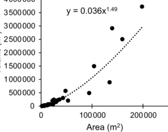
In order to assess the severity of potential GLOF events, lake volumes were estimated using an empirical relation-ship between lake area and volume derived from bathymet-ric measurements of 32 Type 1 and Type 2 lakes, with ar-eas ranging between 2000 and 200 000 m2, in the Zailiiskiy Alatau and Djungarskiy Alatau in 2009–2014 at the end of the ablation seasons in late August–September (Medeu and Blagoveshenskiy, 2015). In these surveys, lake depth was measured using echo sounding conducted along the multiple profiles spaced at approximately 10 m with the along-profile
y = 0.036x1.49 0 500000 1000000 1500000 2000000 2500000 3000000 3500000 4000000 0 100000 200000 Vo lu me (m 3) Area (m2)
Figure 5. Relationship between lake area and volume in the Zaili-iskiy and Djungarskiy Alatau.
increment of 3–5 m. The values of lake volumes were derived from the depth measurements using Surfer software. The high-density depth measurements of each lake enabled rep-resentation of complex lake morphometries which are often neglected in lake area–volume scaling (Cook and Quincey, 2015). The relationship between volumes and areas of the surveyed lakes is shown in Fig. 5 and is approximated by the Eq. (1)
V =0.036 · A1.49, (1)
where V (m3)is lake volume and A (m2)is lake area. This re-lationship is almost identical to that quoted by Evans (1986) for the ice-dammed lakes in Canada. Peak discharge was es-timated using the relationship between lake volume and dis-charge of Haeberli (1983):
Qmax=2V /t, (2)
where V is volume calculated using Eq. (1) and t is time equalling 1000 s. Peak discharge was calculated for the indi-vidual lakes which were identified as potentially hazardous. While peak discharge represents the worst-case scenario ex-pected from a sudden and complete drainage of individual lakes, which is unlikely in the case of larger lakes, it does not account for potential drainage of cascades of multiple lakes as observed in the region in the 1970–1980s.
3.6 Modelling glacier bed topography and detection of overdeepenings
Here we use the glacier bed topography version 2 (GlabTop2) model to derive glacier bed topography based on glacier sur-face slope. GlabTop2 is fully described in Frey et al. (2014) and is based on the same concept as the original GlabTop model (Linsbauer et al., 2012). Both models assume a con-stant basal shear stress along the central flow line of an entire glacier. Ice thickness is then calculated according to
h = τ
f · ρ · g ·sin α, (3)
where h is ice thickness (m), τ is basal shear stress, f is shape factor (0.8), ρ is ice density (900 kg m−3), g is accel-eration due to gravity (9.81 m s−2)and α is glacier surface slope. The basal shear stress is estimated from an empiri-cal relationship between τ and glacier height extent 1z (i.e. maximum elevation minus elevation of the glacier tongue) according to Haeberli and Hölzle (1995). Here we calculated 1zusing the elevation z of the lowest and highest grid cells that fall within each glacier polygon.
GlabTop2 is fully automated, entirely grid-based and first calculates the ice thickness at a set of randomly selected grid areas. Subsequently, these thickness values are interpolated to the entire glacier area. To achieve realistic glacier cross sections, the interpolation scheme assigns a minimum, non-zero ice thickness to all grid cells directly adjacent to the glacier margin. The method includes some non-physical, tun-able parameters such as the density of the random point sam-pling (see Frey et al., 2014, for a detailed description and discussion).
To calculate the glacier bed topography of all glaciers in the Djungarskiy Alatau, identical settings as in Frey et al. (2014) were used. Ice thickness distribution for all glaciers larger than 0.1 km2 has been calculated based on the out-lines of glaciers as in 2000 generated as part of regular cat-aloguing of glaciers of Kazakhstan (Severskiy et al., 2016) and SRTM DEM surface topography. To reduce the influence of small-scale surface undulations in the ice thickness mod-elling, SRTM DEM with 30 m resolution was down-sampled to 75 m cell size.
Overdeepenings in the glacier beds, where future lakes may develop, were identified following the methodology outlined in Linsbauer et al. (2012, 2016) – namely a sink fill algorithm available in ARC GIS 10.4 was run on the modelled bed topography to create a sink-filled version of DEM and the original bed topography DEM was subtracted from the sink-filled version. The difference grid between the filled DEM and the initial DEM without glaciers resulted in a bathymetry raster of the overdeepenings. The follow-ing morphometric characteristics of overdeepenfollow-ings were de-rived: area, maximum and mean depth, volume, maximum length, maximum width (perpendicular to the longest line), and elongation (width-to-length ratio) following Linsbauer et al. (2016) and Haeberli et al. (2016). Overdeepenings with individual areas larger than 11 000 m2, corresponding to the area of approximately two grid cells in the glacier bed topog-raphy, were considered to exclude potential model artefacts in line with previous studies (Linsbauer et al., 2012; Haeberli et al., 2016).
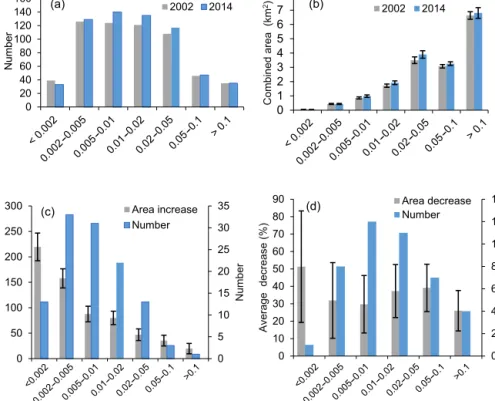
0 20 40 60 80 100 120 140 160 Nu mbe r (a) 2002 2014 0 1 2 3 4 5 6 7 8 Co mbi ne d are a (km 2) (b) 2002 2014 0 5 10 15 20 25 30 35 0 50 100 150 200 250 300 Nu mbe r Ave rag e in crea se ( %) (c) Area increase Number 0 2 4 6 8 10 12 14 0 10 20 30 40 50 60 70 80 90 Nu mbe r Ave rag e de crea se (%) (d) Area decrease Number
Figure 6. (a) Number of lakes, (b) their combined areas, relative change in lake areas averaged over size category, and number of lakes whose areas (c) increased and (d) decreased. The x axes show size categories (km2). The vertical bars represent the uncertainty of measurements. Note that different scales are used in (c) and (d).
4 Results
4.1 Characteristics of lakes and their distribution In 2002 and 2014, 599 lakes with a combined area of 16.26 ± 0.85 km2 and 636 lakes with a combined area of 17.35 ± 0.92 km2 respectively were identified. In 2002, the largest measured lake area was 1.03 km2, the small-est was 0.0007 km2 and the mean was 0.027 km2. Lakes with individual areas of 0.002–0.05 km2prevailed, account-ing for 80 % by number and 42–45 % of the combined area (Fig. 6a, b).
The lakes were positioned within the elevation bands of 2220–3660 and 2220–3690 m in 2002 and 2014 respectively. The small shift of the upper boundary of 30 m is larger than the absolute vertical accuracy of SRTM GDEM of ±10 m, but we note that the latter was derived from a small number of GCPs (Sect. 3.1). The majority of lakes (60 and 56 %), accounting for 56 and 52 % of their total combined area in 2002 and 2014 respectively, were positioned between 3100 m and 3400 m a.s.l. (Fig. 7).
The Type 3 lakes prevailed by both number and combined area followed by the Type 2 lakes (Table 2). There were rel-atively few Type 4 lakes, but their individual areas were an order of magnitude larger, averaging 0.11 km2than the other types of lakes. Type 4 lakes were positioned at lower eleva-tions and, for this reason, the average lake size within the
0 2 4 6 8 10 2200–2500 2500–2800 2800–3100 3100–3400 3400–3700 Combined area (km2) 2002 2014 m a.s.l. 11 9 7 7 358 362 144 162 79 96
Figure 7. Lake count (numbers) and combined area (bars) by el-evation (m a.s.l.). The black bars represent the uncertainty of area measurements.
lowest elevation range of 2200–2500 m a.s.l. was 0.2 km2, which is higher than in any other elevation band.
The largest number of lakes with the highest total com-bined area occurred in the catchments of the rivers Usek, Koksu and Aksu, of which the first two are the largest catch-ments in the study area (Table S2; Fig. 1). The average size of the lakes in these catchments was 0.023–0.036 km2. Larger
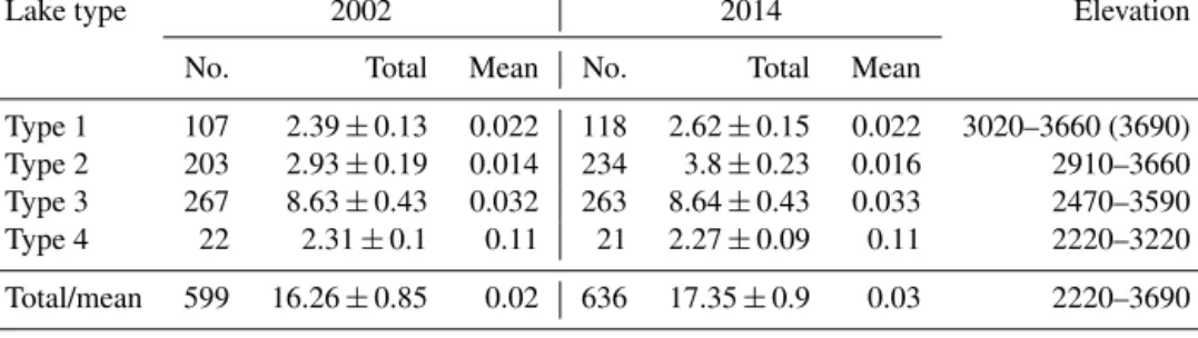
Table 2. Distribution of lakes by type in 2002 and 2014. Lake areas (combined and mean) are in km2; elevation is in m a.s.l. Elevation given in parentheses refers to 2014.
Lake type 2002 2014 Elevation
No. Total Mean No. Total Mean
Type 1 107 2.39 ± 0.13 0.022 118 2.62 ± 0.15 0.022 3020–3660 (3690) Type 2 203 2.93 ± 0.19 0.014 234 3.8 ± 0.23 0.016 2910–3660 Type 3 267 8.63 ± 0.43 0.032 263 8.64 ± 0.43 0.033 2470–3590
Type 4 22 2.31 ± 0.1 0.11 21 2.27 ± 0.09 0.11 2220–3220
Total/mean 599 16.26 ± 0.85 0.02 636 17.35 ± 0.9 0.03 2220–3690
lakes with mean areas of 0.04 and 0.062 km2 were char-acteristic the Khorgos and Lepsy catchments respectively. The number and combined area of lakes in 15 catchments as in 2002 (Table S2) correlated closely with the number of glaciers (correlation coefficients of 0.86 for both) and with the combined glacierized area (0.67 and 0.72 respectively) (Table S1).
4.2 Changes in the number and characteristics of the lakes
Between 2002 and 2014, the overall number of lakes creased by 6.2 %. While areas of 19.5 % of the lakes in-creased, areas of 12.5 % of the lakes declined, including those lakes that have drained completely (Table 3; Fig. 6c, d). Changes in 68 % of all the lakes (as in 2002) were within the uncertainty of measurement.
Figure 6 illustrates changes in areas and abundance of lakes according to size category. The count of lakes increased in all size categories except the largest (> 0.1 km2), where the count did not change, and the smallest (< 0.002 km2), in which the total number of lakes declined because their areas increased in 2014 in comparison with 2002, and they were assigned to the next size category (Fig. 6a). A small increase in the combined area was observed in all categories too but was close to the uncertainty of measurements (Fig. 6b), and lakes, whose areas either increased (Fig. 6c) or decreased (Fig. 6d) beyond the uncertainty, were analysed separately. The smaller lakes exhibited greater expansion, with the aver-age area of the smallest lakes increasing by 220 % (Fig. 6c). The average area reduction was lower than the increase in all size categories and did not appear to correlate with lake size (Fig. 6d).
The largest increase in abundance and average area, both absolute and relative, characterized Type 1 lakes (Table 4). Out of 44 lakes in the whole sample, which doubled their area, 31 belonged to this type. Out of 69 newly formed lakes, 51 were Type 1 lakes while very few Type 1 lakes decreased in size or drained completely (Table 4). The second largest category exhibiting growth was Type 2 lakes. Although av-erage increase was smaller than that of the Type 1 lakes, their overall numbers and combined area increased by 30 %
(Table 2) due to the transition of 35 lakes from the contact (Type 1) lakes (Table 4). The Type 2 lakes exhibited the most dynamic behaviour as, alongside their growth and formation of new lakes, 12 and 11 % disappeared or decreased respec-tively between 2002 and 2014. The count and area of Type 3 and Type 4 lakes exhibited smaller variations.
Figure 8 shows locations of those lakes whose areas ex-hibited changes exceeding the uncertainty of measurement. The largest number of new lakes and those that increased in size were positioned in the northern and western sec-tors of the Djungarskiy Alatau in the basins of the rivers Aksu (10 % increase in combined area), Bien (14 %), Kora (17 %) and Koksu (11 %) between approximately 3000 m and 3500 m a.s.l. The Koksu catchment accommodates the largest combined glacierized area in the region and the Kora catch-ment is characterized by the highest proportion of glacier-ized area (Table S1). Out of 69 new lakes, 25 formed in these four catchments (Fig. 8c; Table S2). The distribution of lakes whose areas declined was uniform across region and most of these lakes were positioned at slightly lower elevations of 3000–3300 m a.s.l.
4.3 Potentially dangerous lakes
Fifty lakes were identified as potentially dangerous and most are located in the north-western and south-western sectors of the study area (Fig. 1; Table S3). The three largest lakes had individual areas of about 200 000 m2. The area of the second largest lake in the sample (N 5 in the Usek basin) increased by 29 % between 2002 and 2014. The potential worst-case scenario peak discharge of the three largest lakes was es-timated to exceed 5600 m3s−1. Peak discharge of 35 lakes may exceed 300 m3s−1, which was the registered velocity of the flow that devastated the town of Sarkand in 1982 fol-lowing the outburst of Lake Akkol (N 43) positioned 45 km upstream (Tikhomirov and Shevyrtalov, 1985).
The characteristic arrangement of lakes in vertical se-quences or cascades creates the potential for outburst of mul-tiple lakes. Therefore, even small lakes (e.g. six lakes with areas below 20 000 m2; Table S3), which are frequently dis-regarded in GLOF assessments, may be hazardous. Thirty two of the potentially dangerous lakes are part of cascades
Table 3. Changes in number and the combined areas of lakes.
Change 2002–2014 No. Combined area (km2) Change in combined area
2002 2014 km2 %
Increased 116 1.43 ± 0.097 2.41 ± 0.15 0.98 ± 0.26 69 ± 17 Decreased 42 0.68 ± 0.042 0.46 ± 0.03 0.22 ± 0.08 32 ± 17.4 Change within uncertainty 409 13.91 ± 0.7 14.06 ± 0.71 0.15 ± 1.3 1 ± 15.1
New 69 – 0.44 ± 0.03 0.44 ± 0.18 100 ± 15.3
Drained completely 32 0.25 ± 0.02 – 0.25 ± 0.09 100 ± 15.6
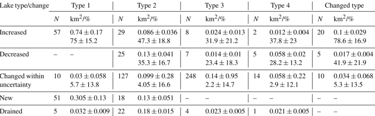
Table 4. Changes in number (N ) and combined area of lakes of different types. For each category, the upper and the lower lines show the absolute (km2)and relative (%) changes respectively. Lakes classified as Type 1 in 2002 and Type 2 in 2014 are shown separately as the “changed type” category.
Lake type/change Type 1 Type 2 Type 3 Type 4 Changed type
N km2/% N km2/% N km2/% N km2/% N km2/% Increased 57 0.74 ± 0.17 75 ± 15.2 29 0.086 ± 0.036 47.3 ± 18.8 8 0.024 ± 0.013 31.9 ± 21.2 2 0.012 ± 0.004 37.8 ± 23 20 0.1 ± 0.029 78.6 ± 16.9 Decreased – – 25 0.13 ± 0.041 35.3 ± 16.7 7 0.014 ± 0.01 23.4 ± 18.3 5 0.058 ± 0.02 28.2 ± 13.2 5 0.017 ± 0.004 41.9 ± 21.9 Changed within uncertainty 10 0.03 ± 0.058 5.7 ± 13.8 127 0.099 ± 0.28 4.05 ± 16.6 248 0.14 ± 0.95 2.2 ± 14.7 14 0.058 ± 0.22 2.9 ± 12.1 10 0.034 ± 0.068 5.3 ± 13.5 New 51 0.305 ± 0.13 18 0.13 ± 0.051 – – – – – – Drained 5 0.032 ± 0.009 22 0.18 ± 0.015 4 0.023 ± 0.005 1 0.021 ± 0.005 – –
of lakes including the two largest lakes in the sample and those in the Aksu (N 45) and Sarkand (N 43) valleys, which burst out in 1970, 1978 and 1982 respectively, causing over-topping of the lakes located at lower elevations. Lake Kap-kan (N 25), identified as dangerous and the only lake in the Djungarskiy Alatau that has been periodically lowered since August 2014, belongs to a cascade of six lakes. Four of those lakes (not identified as potentially dangerous by themselves), including Lake Boskol (Type 3) with an estimated volume of about 5.34 × 10⁵m3and Lake Kazaknkol (Type 4; Fig. 4d) with an estimated volume of 6 × 10⁶m3, are located at lower elevations on the potential flow path to the town of Khorgos hosting the recently established International Trade Centre (Medeu et al., 2013).
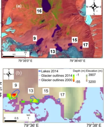
Lakes N 15 (Type 1) and 17 (Type 2; 72 % increase) in the Aksu catchment are positioned at the top of the largest cas-cade of lakes in the Djungarskiy Alatau (Figs. 3 and 9a). The largest lake (N 16) in this cascade has an area of 185 000 m2. The outburst of Lakes 15 ad 17 can potentially cause over-topping of Lake 13, whose area increased by 121 % between 2002 and 2014, reaching 67 000 m2. The outburst of Lake 13 and Lake 9, whose area increased between 2002 and 2014 by 57 %, reaching 68 825 m2, can trigger, in the worst-case sce-nario, an outburst of four downstream lakes with a combined area exceeding 340 000 m2.
A number of large cascades consisting of multiple lakes are positioned in the basin of the river Bien. Figure 10 shows a cascade comprised by four lakes of Types 1 and 2 with a combined area of 119 300 m2. A contact Lake N 22, posi-tioned at the top of the cascade, formed after 2002, reaching 44 200 m2 in 2014, and has potential for further expansion (Sect. 4.4; Fig. 10b). In the Bien basin, the downstream in-frastructure and farmland are located within 23–30 km from the potentially dangerous lakes, which is closer than in other regions.
4.4 Ice thickness modelling and detection of overdeepenings
4.4.1 Ice thickness calculation
Ice thickness distribution for all glaciers larger than 0.1 km2 has been calculated based on the glacier outlines for 2000 and the SRTM DEM surface topography with the original 30 m spatial resolution resampled to 75 m resolution. The to-tal calculated ice volume in the Djungarskiy Alatau amounts to 29 km3. Average modelled ice thickness is relatively shal-low at 33 m; maximum ice thickness reaches 197 m. Both values reflect the fact that the glaciers of the Djungarskiy Alatau are mostly small mountain valley or cirque glaciers. To our knowledge, no ice thickness measurements have been
Figure 8. Spatial distribution of lakes which (a) increased in size, (b) decreased in size, (c) newly formed and (d) drained completely.
carried out in the Djungarskiy Alatau besides the extensive helicopter-borne measurements on 103 glaciers in 1981, pub-lished by Macheret et al. (1988). However, the hand-drawn maps and sketches of ice thickness distribution, shown in the aforementioned study, only allow for a qualitative compari-son with our model results. We find that the measurements and our model results agree on relatively thin glaciers with maximum ice thicknesses of typically around 80 to 120 m and rarely exceed 150 m. The qualitative comparison agrees with the more quantitative evaluations where GlabTop2 has been shown to be well suited for mountain glaciers (Frey et al., 2014, Farinotti et al., 2017).
An extensive model intercomparison exercise (Farinotti et al., 2017) has compared ice thickness measurements from various glaciers to a variety of different modelling ap-proaches that all calculate ice thickness based on glacier surface properties. The study has shown that for mountain glaciers both GlabTop and GlabTop2 perform similar to other approaches. The intercomparison exercise also showed that an uncertainty of ±30 % in modelled ice thickness, earlier es-tablished for GlabTop (Linsbauer et al., 2012) and GlabTop2 (Frey et al., 2014), is fairly typical for all modelling ap-proaches. We thus suggest adopting the same uncertainty for
the present modelling of the ice thickness distribution in the Djungarskiy Alatau.
In the context of this study, it would be of particular inter-est to compare modelled and measured overdeepenings un-derneath glacier tongues. However, Macheret et al. (1988) indicate lacking bed returns on the termini of the vast major-ity of the measured glaciers, making such a comparison vir-tually impossible. Instead, we analyse whether some of the overdeepenings modelled underneath glacier termini in 2000 have developed into actual lakes by the year 2014.
4.4.2 Detection of overdeepenings and potential development of lakes
A total of 513 overdeepenings with individual areas in ex-cess of 11 000 m2were detected in the modelled glacier beds within the glacierized area as in 2000. Their combined area was estimated as 14.7 km2, which corresponds to 3 % of the total glacierized area (Table S1).
Most overdeepenings are small and shallow with length and width of a few hundred metres and maximum depth of 65 m (Fig. 11). The individual areas of 96 % of all overdeep-enings are less than 0.1 km2. Larger overdeepenings with in-dividual areas between 0.05 and 0.5 km2 are found in the regions where existing lakes are most abundant (the Aksu,
Figure 9. (a) Cascade of lakes in the Aksu basin (Landsat scene from 2014) and (b) modelled overdeepenings using the glacier mask from 2000 and actual lakes as in 2014.
Usek and Khorgos basins), but also in the north-east of the region where the existing lakes are small and currently less numerous, but where new lakes develop and the existing ones show rapid (over 100 %) increase (Fig. 8a, c). The mean vol-ume is 0.33 × 10⁶m3, and this is close to the mean volume of 32 Type 1 and Type 2 lakes (whose bathymetry was mea-sured; Sect. 3.5) of 0.47 × 10⁶m3.
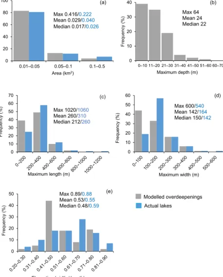
Frequency distributions, mean and median values of the selected morphometric parameters of the modelled overdeepenings were compared to those of 134 Type 1 and Type 2 lakes with areas in excess of 11 000 m2 as in 2014 (Fig. 11). The frequency distributions of areas of the mod-elled overdeepenings and existing lakes are very similar; however, both mean and median areas of the overdeepenings are smaller than those of the lakes (Fig. 11a). The major-ity of the existing lakes have maximum lengths and widths of 200–400 and 100–200 m respectively, and their width-to-length ratio (elongation) peaks at 0.6–0.8, pointing to a lower eccentricity in line with the prevalence of the cirque glaciers in the region currently and in the past (Vilesov et al., 2013). While the frequency distribution of the maximum length val-ues is replicated by the model, the majority of the modelled overdeepenings tend to be narrow, probably because most overdeepenings are small. Thus elongation of 44 % of the overdeepenings is within a 0.4–0.5 range (Fig. 11e), while
Figure 10. (a) Cascades of lakes in the Bien River basin (Land-sat scene from 2014) and (b) modelled overdeepenings using the glacier mask from 2000 and actual lakes as in 2014.
areas of 38 % of the overdeepenings do not exceed that of two model grid cells.
The locations and characteristics of overdeepenings were analysed with regard to the lakes formed within the as-sessment period in the de-glacierized area. All actual lakes, including those smaller than 11 000 m2, were considered. Overall, 66 actual lakes (56 new and 10 whose formation began earlier) were identified within this domain ranging in size between 960 m2and 44 260 m2. Within the same area, 148 overdeepenings were identified (116 within the fully de-glacierized area). Positions of 44 overdeepenings coincided with positions of the actual lakes – i.e. 67 % match. The mean and median areas of these overdeepenings were 60 600 and 39 400 m2respectively.
Not all overdeepenings will become lakes, as those that are smaller and shallow will be filled by sediment (Linsbauer et al., 2012, 2016). In this study, 72 overdeepenings were iden-tified as “false positives”, e.g. no lakes formed in place of the identified overdeepenings following the complete retreat of glaciers by 2014. The remaining overdeepenings were within the partially de-glacierized area where lakes can potentially develop. Most of the false positive overdeepenings were shal-low (maximum depth less than 25 m) and small with individ-ual areas less than 0.05 km2and mean and median areas of
0 20 40 60 80 100 0.01–0.05 0.05–0.1 0.1–0.5 Frequ en cy (%) Area (km2) (a) Max 0.416/0.222 Mean 0.029/0.040 Median 0.017/0.026 0 10 20 30 40 0–10 11–20 21–30 31–40 41–50 51–60 60–70 Frequ en cy (%) Maximum depth (m) (b) Max 64 Mean 24 Median 22 0 10 20 30 40 50 60 70 Frequ en cy (%) Maximum length (m) (c) Max 1020/1060 Mean 260/310 Median 212/260 0 10 20 30 40 50 60 Frequ en cy (%) Maximum width (m) (d) Max 600/540 Mean 142/164 Median 150/142 0 10 20 30 40 50 Frequ en cy (%)
Elongation (width / length)
(e) Max 0.89/0.88 Mean 0.53/0.55 Median 0.48/0.59 Modelled overdeepenings Actual lakes
Figure 11. Histograms of the selected parameters of 513 modelled overdeepenings and 134 actual Type 1 and Type 2 lakes with areas in excess of 11 000 m2as in 2014: (a) area (km2); (b) maximum depth (m); (c) maximum length (m); (d) maximum width (m); (e) elongation (width to length ratio).
18 900 and 16 875 m2. The areas of 50 % of the false positive overdeepenings were at the imposed threshold of two grid cells.
Figure 10b shows an overdeepening with the largest area in the data set is positioned at the top of a cascade of lakes in the Bien River basin identified as in danger of GLOF. In the worst-case scenario, filled to the brim, this overdeepen-ing may contain 9.4 × 10⁶m3 of water, which exceeds the volume of Lake Kapkan, the only artificially lowered lake, approximately by a factor of 3. At the exact site of this overdeepening, modelled using the glacier mask from the year 2000, Lake 22 formed and increased rapidly between 2002 and 2014 (Fig. 10b; Table S3; Sect. 4.3), and its area could potentially increase by an order of magnitude in the fu-ture. In the Aksu basin, the formation and growth of Lakes 9 and 13 (by 57 and 123 % respectively) coincided with the modelled overdeepenings; however, modelling suggests that
the potential for the increase in Lake 13 is limited (Fig. 9). Similarly, limited expansion is projected for Lake Kapkan (N 25) although multiple overdeepenings with individual areas between 40 000 and 70 000 m2were identified in its vicinity, suggesting that new lakes may form (not shown). Lake Akkol (N 43) is not expected to increase according to the results of modelling, and, indeed, the lake area did not change between 2002 and 2014 (Table S3).
5 Discussion
5.1 The inventory and evolution of lakes
This study assessed changes in approximately 600 un-managed lakes in the Djungarskiy Alatau between 2002 and 2014 with regard to various types and size classes of lakes and characteristics of the catchments. The
over-all number of lakes increased between 2002 and 2014 by 6.2 % (0.51 % a−1). The combined areas increased from 16.26 ± 0.85 to 17.35 ± 0.92 km2and the overall change was within the uncertainty of measurements. These results are comparable to the increase of 7 % (0.7 % a−1)in lake count and area presented by Wang et al. (2013) for a wider re-gion of the northern Tien Shan for the 2000–2010 period. The difference between the two studies is close to the un-certainty of measurements and can be attributed to the dif-ference between methodologies (automated versus manual mapping) and lake size distributions in the samples. Narama et al. (2010b) reported a smaller increase in the area of 36 lakes in the Terskey Alatoo in the 1998–2008 period, attribut-ing it to the comparatively slow glacier retreat in the region.
The overall increase in both count and area is relatively small. This is partly because the sample is dominated by small lakes for which uncertainty is higher, and we consider changes in 68 % of all lakes to be within the uncertainty of measurements. In this study, 7, 17 and 24 % of lakes were smaller than the thresholds of 2000, 3600 and 4500 m2 ap-plied by Wang et al. (2013), Gardelle et al. (2011) and Li and Sheng (2012) respectively in their assessments of changes in lake areas in the Tien Shan, Hindu Kush and Himalayas. Another reason is a dynamic behaviour of the lakes. In con-trast to changes in the area of glaciers, which retreated in the region during the 2000s (Severskiy et al., 2016; Table S1), both the expansion and formation of lakes and their drainage were registered, and the average statistics conceals signifi-cant variations.
In the subsample of lakes whereby changes exceeded the uncertainty of measurements, the increase in lake count and area dominated over reduction. The areas of 116 lakes in-creased and 69 new lakes formed, while areas of 42 lakes decreased and 32 lakes drained completely (Table 2; Fig. 6). Similar diversity in lake evolution and rates between increas-ing and decreasincreas-ing numbers of lakes was reported by Li and Sheng (2012) for the Himalayas. The largest increase in lake count characterized Type 1 (contact) lakes (Table 4), and sim-ilar results were reported by Wang et al. (2012) and Gardelle et al. (2011) for the Hindu Kush and the Himalayas. The Type 2 lakes, developing on the young moraines, were the second largest group exhibiting growth; however, the most active reduction in lake area was also registered in this sub-set, usually following glacier retreat and separation between lakes and glacier tongues.
In comparison with other regions of the Tien Shan, the number of lakes increased marginally faster in the Djun-garskiy Alatau than in the western and central Tien Shan, where the abundance of lakes was growing at a rate of 0.4 % a−1, but slower than in the eastern Tien Shan, where the increase in the number of lakes reached 1.7 % a−1 be-tween 2000 and 2010 (Wang et al., 2013). The increase in combined area was marginally higher than in the western Tien Shan but lower than in its central and eastern sectors (Wang et al., 2013). The growing numbers and areas of lakes
in the glacierized regions contrasted strongly with the evo-lution of lakes on the adjacent plains where the large-scale atmospheric circulation controls (and subsequently variabil-ity in temperature and precipitation) are the same but glacier melt does not contribute to lake nourishment. Thus during 1987–2010, on the plains of Mongolia, the number of lakes with individual areas in the range of 1–10 km2and their com-bined area decreased by 10.5 and 28 % respectively follow-ing a strong increase in evaporation (Tao et al., 2015). 5.2 The observed climate and glacier change and lake
evolution
The evolution of lakes resulted from a combination of the following factors: (i) climatic changes including changes in temperature and the difference between precipitation and potential evaporation (PET), (ii) glacier melt nourishing lakes, (iii) melt of buried ice and permafrost affecting both lake nourishment and drainage, and (iv) local topography and stability of moraines supporting the lakes. Contributions of these factors vary between lake types, temporally and spa-tially.
There are no high-altitude meteorological stations with continuous records in the study area; however, significant positive temperature trends were identified at the stations lo-cated between approximately 600 and 1700 m a.s.l. in all sea-sons, including the summer ablation season. The JJA tem-peratures were increasing at a rate of 0.18◦C per decade be-tween 1960 and 2014 at the regional stations (Fig. 1) with lin-ear trends, which is significant at the 95 % confidence level, explaining approximately 20 % of the variance in the data set. Positive trends in summer temperatures are observed across the Tien Shan (Kutuzov and Shahgedanova, 2009; Narama et al., 2010a; Wang et al., 2013). Vilesov et al. (2013) estimated PET for the Mynzhylki meteorological station (3010 m a.s.l.) in the Zailiiskiy Alatau, concluding that, while the long-term record exhibits a statistically significant positive trend con-sistent with temperature increase, the change in PET between the 1990s and 2000–2010 was small (about 5 % of the annual mean). Trends in precipitation vary between the mountainous regions of Central Asia (Kutuzov and Shahgedanova, 2009; Narama et al., 2010a; Wang et al., 2013), but in the foothills of the Djungarskiy Alatau as well as at the high-elevation stations of the Zailiiskiy Alatau neither annual nor summer precipitation exhibited statistically significant trends both be-tween 1960 and 2014 and within the assessment period. We suggest that changes in effective precipitation (difference be-tween precipitation and PET) were not the main control over lake evolution in the Djungarskiy Alatau in contrast to the adjacent plains (Tao et al., 2015).
Glacier mass balance is a useful predictor of lake evo-lution (Gardelle et al., 2011; Wang et al., 2015). While no continuous records exist for the assessment period in the Djungarskiy Alatau, mass balance records from the Tuyuksu glacier in the Zailiiskiy Alatau show predominantly
nega-tive annual and strongly neganega-tive cumulanega-tive mass balance (Severskiy et al., 2016). The mass balance data derived from GRACE and ICESat (Farinotti et al., 2015) show that val-ues of negative mass balance in the Djungarskiy Alatau are close to those observed in the Zailiiskiy Alatau and indicate a mass loss of approximately −0.5 × 10³kg m−2a−1. As a result, between 2002 and 2014 glaciers lost between 5 and 30 % of their combined area (Table S1), contributing to the expansion of particularly contact Type 1 lakes, 73 % of which increased, and 51 new lakes formed (Table 4).
Degradation of buried ice and permafrost controls both growth and rapid discharge of morainic lakes as GLOF events often result from buried ice erosion and moraine dam instability (Jansky et al., 2010; Evans and Delaney, 2015). By contrast, Severskiy et al. (2013) noted that many morainic lakes that existed in the 1970s gradually disappeared in the 21st century because of thawing of permafrost (Severskiy, 2009). Permafrost originally formed an impermeable layer on which lakes developed, but, as it thawed, the active for-mation of underground drainage channels enabled gradual drainage of the lakes. Field surveys revealed the widespread presence of buried ice in the contemporary moraines in the Djungarskiy Alatau, where Type 2 lakes develop, but not in the LIA and older moraines, where Type 3 lakes occur (Vilesov et al., 2013). This difference might explain the small changes in Type 3 lakes over the relatively short period of time and more dynamic behaviour of Type 2 lakes (Table 4). The effect of melting permafrost on dam stability can be monitored using multi-temporal high-resolution satellite im-agery and DEMs (Fujita et al., 2008; Narama et al., 2010b; Bolch et al., 2011; Petrov et al., 2017), and this analysis will be performed in the future.
5.3 Risks of lake outbursts and modelling of overdeepenings in glacier beds for hazard management
GLOF events peaked in the Djungarskiy and neighbouring Zailiiskiy Alatau between 1975 and 1984 (Fig. 12) when strong positive JJA temperature anomalies and enhanced glacier melt were observed. The frequency of GLOF was lower in the late 1980s when glacier retreat was slower and when management of lakes was introduced in the more densely populated Zailiiskiy Alatau (Severskiy et al., 2013). Despite these efforts, two GLOF events occurred in 2014 and 2015 in the Zailiiskiy Alatau following strongly posi-tive JJA temperature anomalies of 2–3◦C (reaching 6◦C in
July 2015) recorded at the Tuyuksu meteorological station (3440 m a.s.l.). In August 2014, periodic artificial lowering of Lake Kapkan commenced in the Djungarskiy Alatau to prevent its outburst.
Fifty lakes, whose outburst can potentially pose a threat to existing infrastructure, were identified (Table S3) as a first step in the assessment of GLOF risk. Most are large enough to cause damage in the case of an outburst of a single lake;
0 1 2 3 4 5 6 7 8 9 1952 1955 1958 1961 1964 1967 1970 1973 1976 1979 1982 1985 1988 1991 1994 1997 2000 2003 2006 2009 2012 2015 Nu mbe r of GLOF Year
Djungarskiy Alatau Zailiyskiy Alatau
Figure 12. GLOF events attributed to an increase in air tempera-ture and melt (as opposed to precipitation), which resulted in the recorded damage to housing and infrastructure in the Zailiiskiy and Djungarskiy Alatau. The data before 1985 are from Popov (1986); data for the later years were provided by KSAMP.
however, smaller lakes can pose a danger due to their po-tential to trigger overtopping of lakes located downstream. Many lakes exhibited strong growth within the assessment period (Tables 4; S3) and are projected to increase in the fu-ture. The use of the most stringent criteria derived from the previous GLOF events, literature and empirical models (e.g. peak discharge resulting from the worst-case scenarios) im-plies that anticipated floods are low probability events, and further justification through physical modelling of floods and mudflows and field surveys, focusing on the state of lake dams, is required. An example, where further modelling of potential floods is needed to constrain uncertainty and as-sist planning, is the basin of the Bien River, where a rapid increase in newly formed lakes is observed, comparatively close to the existing infrastructure, and their further increase is projected to potentially result in the formation of one of the largest lakes in the region (Fig. 10b).
Results of modelling of outburst paths and mass move-ments depend on the quality of GDEMs. The average differ-ence between SRTM and ASTER GDEM was approximately 4◦ for the slopes surrounding lakes with steeper slopes de-rived from ASTER GDEM (Sect. 3.4). A detailed compari-son of two GDEMs and their validation will require extensive ground truth data which are currently unavailable. Due to the stringent criteria applied to the selection of dangerous lakes (i.e. distance to the infrastructure and average incline along the potential flood path line), the DEM uncertainty does not affect the “first-order” identification of dangerous lakes pre-sented here. However, a more accurate DEM and evaluation of its quality may be required for modelling debris flow prop-agation.
Modelling future evolution of dangerous lakes, based on the identification of overdeepenings in the modelled glacier beds, may be used to inform hazard management and plan-ning. Previous studies have shown that while simulation of
locations of overdeepenings is robust (Frey et al., 2014; Lins-bauer et al., 2012, 2016), their morphometry is subject to considerable uncertainty (Haeberli et al., 2016). A compar-ison of the morphometry of the overdeepenings in the Djun-garskiy Alatau with that of the existing lakes (Fig. 11) shows that their parameters, including mean statistics and frequency distributions, are close, providing a degree of confidence in the simulations. The frequency of slightly larger areas (0.05– 0.1 km2)is higher in the modelled sample, but both samples show that very small lakes (0.01–0.05 km2)prevail. Narrow overdeepenings, under 100 m in width, are most frequent (44 %), while the majority of actual lakes (57 %) are 100– 200 m wide (Fig. 11d). This discrepancy is likely to be an artefact of a large number of small (two grid cell) overdeep-enings in the sample. As a result, oval-shaped overdeepen-ings with elongation of 0.4–0.5 prevail while actual lakes tend to have a more circular form.
A comparison with the morphometries modelled for the Swiss Alps, Himalaya–Karakoram region and Peruvian Cordillera Blanca (Haeberli et al., 2016) shows that ar-eas of the overdeepenings in the Djungarskiy Alatau are smaller than in all three regions, in line with the smaller size of glaciers. Maximum depth statistics are comparable with those for the Himalaya–Karakoram region and the Cordillera Blanca. Shallow overdeepenings, with a maximum depth less than 50 m, dominate in all regions and in the study area; max-imum depth values are less than 40 m for 95 % of all identi-fied overdeepenings.
A correct simulation of locations of overdeepenings is im-portant in application to hazard management. Our compar-ison of locations of the contact lakes, formed since 2000, with modelled overdeepenings showed that locations of 67 % of the lakes were simulated correctly although the number of false positives was high. Following the analysis of phometries of the false positives and a comparison of mor-phometries of the existing lakes and the overdeepenings (e.g. width and elongation, Fig. 11), we recommend that a thresh-old of 20 000 m2is applied to identify overdeepenings which are likely to provide sites for the development of lakes, as 85 % of the actual lakes formed in the overdeepenings with areas larger than 20 000 m2.
A promising outcome of this investigation is a good agree-ment between the simulated areas of overdeepenings and the observed evolution of the lakes. For example, areas of two lakes, the Kapkan (prior to its artificial lowering) in the Khor-gos basin and Akkol in the Sarkand basin, currently consid-ered by KSAMP as the most dangerous in the region, did not increase between 2002 and 2014 and modelling suggests that they already have filled overdeepenings in the terrain. However, a strong growth of Lake 22 in the Bien catchment (Table S3) occurred in place of the largest of the identified overdeepenings (Fig. 10b). These and other (e.g. formation of multiple lakes in larger overdeepenings) examples suggest that the GlabTop modelling approach is a useful tool for plan-ning and hazard management.
6 Conclusions
An increase in abundance and combined area of mountain lakes was observed in the Djungarskiy Alatau between 2002 and 2014. The overall change was moderate at approximately 6 %; however, the small overall increase resulted from a very dynamic behaviour of lakes which involved both growth and drainage of lakes over time. Two categories of lakes, those developing on the young moraines and contact lakes, exhib-ited the strongest growth, which agreed well with projected areas of overdeepenings in the subglacial topography simu-lated using the GlabTop2 model. Fifty existing lakes were identified as potentially dangerous. In the future, the signif-icance of hazard potential of these lakes will be assessed trough further investigation of lake dams and surrounding slopes using high-resolution remote sensing and field stud-ies and physically based flow models.
Over 500 overdeepenings in the glacier beds were iden-tified using the GlabTop2 model, with the highest number in the Aksu, Bien and Kora basins in the north-west and Lepsy basin in the north-east of the region. A comparison of locations of the modelled overdeepenings and actual lakes formed within the recently de-glacierized area shows that GlabTop2 can serve as a useful tool in hazard management in the region. The application of an area threshold of 20 000 m2 to the identified overdeepenings may help to reduce the num-ber of overdeepenings which are unlikely to provide sites for lake formation. The uncertainties in modelling and the ongoing development in the region imply that the observed and modelled evolution of the lakes should be regularly re-assessed against each other and against changes in land use and infrastructure to inform hazard management and plan-ning.
Data availability. Data on the potentially dangerous lakes are pre-sented in the Supplement (Table S3). The original shape files of the lakes can be obtained from the University of Reading Re-search Data Archive (https://reRe-searchdata.reading.ac.uk/, Kapitsa and Shahgedanova, 2017).
The Supplement related to this article is available online at https://doi.org/10.5194/nhess-17-1837-2017-supplement.
Author contributions. MS designed the study, contributed to data analyses (identification of overdeepenings; statistical analysis) and wrote the text; VK carried out lake mapping and identification of potentially dangerous lakes, and contributed to the statistical anal-ysis; HM ran the GlabTop2 model and contributed to writing the text; IS and AM contributed to the study design and discussion of the results.