Distributed detection and coding in information networks

(1)

Distributed Detection and Coding in Information

Networks

by

Shan-Yuan Ho

Submitted to the Department of Electrical Engineering and Computer

Science in partial fulfillment of the requirements for the degree of

Doctor of Philosophy

at the

MASSACHUSETTS INSTITUTE OF TECHNOLOGY

February 2006

©

Shan-Yuan Ho. All rights reserved.

The author hereby grants to MIT permission to reproduce and

distribute publicly paper and electronic copies of this thesis document

in whole or in part.

A uthor ...

M^ASCUES ISITUTE.

O.TECHNOLOGY

..

J.RARIES

Department of Electrical Engineering and Computer Science

January 31, 2006

Certified by...

. . . .

.Robert G. Gallager

Professor of Electrical Engineering and Computer Science

Accepted by ...

.

...

-Thesis Supervisor

A

r C.

...

i...

Arthur C. Smith

Chairman, Department Committee on Graduate Students

MA _{SSACHUET INS} E

COF TECHNOLOGY

r

(2)

Distributed Detection and Coding in Information Networks

by Shan-Yuan Ho

Submitted to the Department of Electrical Engineering and Computer Science on January 31, 2006, in partial fulfillment of the

requirements for the degree of Doctor of Philosophy

Abstract

This thesis investigates the distributed information and detection of a binary source through a parallel system of relays. Each relay observes the source output through a noisy channel, and the channel outputs are independent conditional on the source input. The relays forward limited information through a noiseless link to the final destination which makes an optimal decision. The essence of the problem lies in the loss of information at the relays. To solve this problem, the characteristics of the error curve are established and developed as a tool to build a fundamental framework for analysis. For understanding, the simplest non-trivial case of two relays, each forwarding only a single binary digit to the final destination is first studied. If the binary output constraint is removed and the output alphabet size for one relay is M, then no more than M + 1 alphabet symbols are required from the other relay for optimal operation. For arbitrary channels, a number of insights are developed about the structure of the optimal strategies for the relay and final destination. These lead to a characterization of the optimal solution. Furthermore, the complete solution to the Additive Gaussian Noise channel is also provided.

Thesis Supervisor: Robert G. Gallager

(3)

Acknowledgments

"At times our own light goes out and is rekindled by a spark from another person. Each of us has cause to think with deep gratitude of those who have lighted the flame within us."

- Albert Schweitzer

This is the close of a continuously disrupted and extremely long chapter in my life. Therefore, these acknowledgements are long and yet cannot fully express my gratitude. I am most deeply indebted to my advisor and mentor, Professor Robert G. Gallager. His extreme patience, generosity, and genuine concern for the welfare of his students is unparalleled. Through his mentorship, I received an education in many facets far exceeding the most hopeful expectations of any graduate student. This research experience has been an extraordinary journey, which I have thoroughly enjoyed. I was shown the beauty and style of simplicity in the way of fundamental research and was given the freedom to independently explore my ideas carefully guided by his unprecedented research instinct -where to explore, where to explore further, and when to stop. Few possess a passion for research and even fewer possess the type of deep insight and understanding of both the grand perspective and the minute detail that Prof. Gallager demonstrates. He taught me the clarity of thinking and the profoundity of thought through the simplicity of solution during the research process. He then instructed me in the lucidity and elegance of exposition during the writing process. I was also the beneficiary of Prof. Gallager's wisdom and counsel in various aspects of life, which deeply impacted me. One of the most humble, generous, and honorable people I have ever known, Prof. Gallager's honesty is always stated with graciousness. His example is an inspiration, and his influence has changed my life. I am immensely fortunate to have had the privilege of being a student of Prof. Gallager.

I gratefully acknowledge my committee members from whom I have learned so much: Professor John Tsitsiklis provided invaluable insight, depth of knowledge, and precise statements. I admire his clarity of understanding and brilliance. Professor Emre Telatar gave a meticulous reading of my thesis and enormous help in many ways. His insight, clear explanations, depth of understanding in so many fields, and love of research are exceptional. Professor Daniel Spielman provided astute suggestions and many helpful discussions over the years. A number of other professors have had a signficant influence on my education. I am particularly privileged to have had many enlivening interactions with Professor Daniel Kleitman, and I thoroughly enjoyed both our technical and non-technical discussions. His ability to create valuable learning environments anywhere and to find no problem uninteresting is uncanny. I have learned so many

(4)

tools of the trade and richly benefitted from his remarkable advice and stories. Professor Al Drake was always willing to provide varied input. He included humor in every interaction and understood the soothing of the soul after a long peaceful motorcycle ride. Professor Pierre Humblet first introduced me to the blending of mathematics with engineering in research. His sharp technical insight and kindness is more than appreciated. I thank Professor Yih-Jian Tai for reviving in me my love of literature and history. Through our many scholarly discussions, I felt privileged to to be his student in the modern and classical sense. To Professor Eric Feron who generously gave me his kind help and constant encouragement. To Professor Dimitri Bertsekas for many useful and pleasant interactions. To Professor Martha Gray for her invaluable advice and honest perspective. Professor Dave Forney and Professor Sanjoy Mitter's enthusiasm for research and fruitful interactions have inspired me. To Professor

and Mrs. Vernon Ingram for the generosity of their love and kind support and wise counsel at all times.

I am especially thankful to Marilyn Pierce for her caring support, kindness, and everything she has done for me throughout my graduate career. She took care of every administrative problem that came my way and allowed me to forget the definition of "red tape." The completion of this degree would have been impossible without her. I thank Lisa Bella, Bob Bruen, Peggy Carney, Jennifer Craig, Lisa Gaumond, Michael Lewy, Fifa Monserrate, Kathleen O'Sullivan, Dennis Porche, Peter Swedock for their expert help at needed times.

Many splendid friends, colleagues, and officemates in the Department of Mathematics, Depart-ment of EECS, the Laboratory for Information and Decision Systems, and MIT have contributed richly to my graduate experience, during and beyond.

To Emre Telatar who is the best friend that anyone could possibly ask for, who puts up with my antics at all times, who always provides a listening ear, and who has always been there for me. His sensitivity, graciousness, kindness, humbleness, and integrity have never wavered. To Meng-Yong Goh whose demonstration of utmost loyalty and true friendship since our college days is unsurpassed, for not tiring of hearing my nonsense at all odd hours of the night, and who always has my best interest at heart. I enjoyed my friendship and the many thoughtful discussions with Tom Richardson and Roy Yates and appreciate their honest, down-to-earth perspective, including Roy's sometimes useful advice. Erdal Arikan whose positive

encouragement, advice, and insight is fresh water to a weary soul every time we meet, and whose love of research and learning is infectious. John Keen for his constant encouragement, support and friendship during my roughest times, without a hint of negativity. I had some

(5)

unforgettable officemates who have certainly slowed down the research and dissertation process

but created many fond memories in the meantime. They include Murat Azizoglu, Rick

Barry, Angela Chiu, Ken Chou, Ying Li, Zhi-Quan (Tom) Luo, Muriel Medard,

Rajesh Pankaj, Abhay Parekh, John Spinelli, I.E. Telatar, Paul Tseng, Cynara Wu.

I thank Alex Postnikov for the discourses in mental agility; Diana Dabby for reminding

me that I am still alive; Sanjeev Kulkarni for always keeping an even keel; John Spinelli

and Mark Wang whose humor is unmatched; Rocky Romano for honing me in the art of

procrastination; Chi-Fang Chen whose ability to relax in just about every situation had a

calming effect; Kathy Misovec who frequently questioned my sanity but never doubted my

courage or integrity.

I thank Shelene Chang for her creative and brilliant solutions to some of my

out-of-the-ordinary problems. Tom Klemas

-

fellow coach, instructor, researcher, and student (both

undergrad and grad) for sharing all sorts of thoughts and experiences. We share a rare common

language and ground to talk in breadth and depth. Dan and Lauren Crews and Rita

and John Bonugli for the stress relief and the many delicious home cooked meals. My

good friend Michelle Bonugli for her loyal friendship, hidden talents, unforgettable laughter,

and unrepeatable jokes (which we incessantly repeat anyway!). J.P. Mattia, Paparao, Dana

Pascovici, Richard Stone created many pleasant distractions through this sometimes tedious

ordeal. I have enjoyed the camaraderie of Constantinos Boussios, Randy Berry, Stefano

Casadei, Constantine Caramanis, Emre Koksal, Olivier Leveque, Marina Meila,

Angelia Nedic, Asu Ozdaglar, Anant Sahai, Tengo Saengudomlert, Huizhen Yu.

I am very appreciative of Georgios Kotsalis for his unfailing support, friendship and strength

of character. His insight into people is amazing and his courage and integrity are admirable.

I am also very grateful for the kind understanding, patience, and constant support of Fang

Zhao's friendship and appreciate her kind help with many LA)IX issues in this document,

particularly during the final stages. I will fondly miss the midnight crew of Selcuk Bayraktar,

Georgios Kotsalis, Nuno Martins where the language and topics of conversations were

somehow much more creative than during the day. Fellow instructors, TA's, and former students

(academic and athletic): Andrew Brzezinski, Jenn Cheng, Karolina Corin, Chuying

Fang, Brian Heng, 0. Pat Kreidl, Charlotte Lau, Josh Lifton, Chunmei Liu, Karen

Sachs, David Sachs, Keith Santarelli, Ayanna Samuels, Jolene Singh, Heelo Sudo,

Xiaoyan Xie, Fangyun Yang made my experiences at MIT rich and rewarding.

(6)

Sensei Dick Stroud for teaching me the finer points of harmony, balance and sensitivity, not only on the mat but in life; the MIT fencing team coaches Eric Sollee, Jarek Koniuz, and Rob Hupp, MIT Ice Hockey Team coaches Katia Paskevitch and Tony Gray, for the many hours of instruction, fun, and collegiate competitions. I especially enjoyed many enlightening conversations with my friend and men's gymnastic coach, Noah Riskin. I shall remember members of the MIT Men's Gymnastics Team who provided entertainment and

also helped me with my gymnastics.

A number of wonderful people outside the world of MIT have been especially kind to me. These very special individuals have inspired and supported me at various points during my graduate studies and in my life.

To Master Joe Pina who is the most dedicated and devoted coach that any athlete could ever ask for, who taught me the art of martial art through the sport of Tae-Kwon-Do, and whose in-tense competition training was no less gruesome than any part of my academic education. I had to dig deep within my soul to deliver when I felt there was nothing left to offer. Master Martin Mackowski who is without doubt the finest instructor I have ever had and who built my solid foundation in the basics. To Master Deb Pederson for whom I would have no other coach in my corner during my competitions. To Master Chris Jensen for refining my techniques and basics from the beginning, whose precision and martial analysis is unsurpassed. To my teammates and training partners in California and Massachusetts, thanks for the sweat, pain, and agonizing workouts where we learned that whether sport develops character is questionable,

but one thing we all know for certain, SPORT REVEALS CHARACTER. Many thanks to:

Eric Lee who is without question the finest sparring partner I have ever had and who has pre-pared me for many competitions since our teenage years; World Champions Valery Long who taught me almost everything I know about distancing, timing, and footwork and prepared me firsthand in our many sparring sessions throughout my competitive training; Marcia Hall for the high standards and inspiration; Dana Hee, Deb Pederson, Val Long, Henry Parker, Pedro Xavier, Alberto Montrond, Noel Bennett for the day-in-day-out training and the numerous competitions. Sean Clark whom our coach calls "the World Champion yet to be", whose support, friendship, and loyalty is doubly appreciated. AJ Dunbar the best physical trainer I have come across. Heather Tallman who is perhaps the most diverse and talented individual I have ever met and who has demonstrated that true friendship is timeless.

To my dear friend Dana Hee, Olympic Gold Medalist and Hollywood Stuntwoman, I shall always treasure those sweet memories of intense training, competition, and travel. It was a

(7)

glorious adventure. Since our youth, we deeply share and dearly embrace the invaluable lessons life and experience have taught us. We painfully learned to maximize working with our pre-birth lottery (genetics) in the circumstance of our post-pre-birth lottery (environment) and came to the revelation that no one can take away what is within us.

I am indebted to Kim McGlothin and John Blumenstiel for their expert advice on a variety of issues, pragmatic help at times of crisis, and for teaching me a perspective on human nature that I will carry into the future chapters of my life. I would also like to acknowledge the kind support and insightful understanding of Grace Chiang and Ming-Wen Lu.

I thank my entire medical team at Spaulding Rehabilitation Hospital. Their comprehensive guidance through the rehabilitation process over 3 years helped me rebuild my life after my near fatal accident. This process was extremely painful and trying; however, the support of the entire team gave me hope, comfort, and motivation. I am especially grateful to my Speech Language Pathologist, R. Richard Sanders whose expertise, insightfulness, and patience during our speech therapy sessions were critical to my rehabilitation.

My deep gratitude to Grandpa and Grandma Liu for their warm love and keen interest in all aspects of my life since my youth. I especially thank Grandpa Liu, my maternal grandfather's best friend, for his insightful advice over the years, his deep enthusiasm in all my undertakings, and for always standing behind me in all my pursuits. I am indebted to my Maternal Grandfather for loving me and for believing in me even before I was cognizant of it. His high standards of integrity, fairness, generosity, and strength of character will forever be imprinted on my heart. I thank my sister and brother-in-law, Della and Steve Lau for their help and support at various times.

To my loving Mother for demonstrating a zeal for life, a passion for learning, the courage to endure, for teaching me never to take anything in life for granted, and for instilling in me a love for and appreciation of mathematics. But most of all, for loving me deeply at all times, for always believing in me especially during my lowest times, and for enthusiastically sharing the experiences in all my endeavors. She always patiently listened to me, generously shared her experiences, and provided a keen insight and type of wisdom and understanding that few possess. I will never forget her sacrifices. Her strength of spirit has sustained me, her wisdom has guided me, and her love has nurtured me.

This research is partly supported by a MIT Alumni Fellowship, General Electric Fellowship, MIT EECS Graduate Fellowship, and Grass Foundation Fellowship, and is kindly appreciated.

(8)

Wisdom is supreme; therefore get wisdom.

Though it costs all you have, get understanding.

Turn your ear to wisdom and apply your heart to understanding,

Call out for insight, and cry aloud for understanding,

Look for it as for silver and search for it as for hidden treasure...

Then wisdom will enter your heart and

Knowledge will be pleasant to your soul.

Discretion will protect you and understanding will guard you.

Then you will understand what is right and just and fair

-

every good path.

Preserve sound judgement and discernment,

Do not let them out of your sight;

They will be life for you.

Blessed is the man who finds wisdom, the man who gains understanding,

For she is more profitable than silver and yields better returns than gold;

She is more precious than rubies;

And nothing you desire can compare with her.

(9)

I,

% "m

AZ

4g

t

N-p_ ~7

~)

~~~Ii'

4 L~i~j

~~iN~3

'4;..)

471)

1 --

*

A-44~

0,-4

air

(10)

Dedicated to:

My Honorable and Loving Mother

My Admirable and Respected Professor

The God of the Cosmos

Because they

Supported me during my darkest hours and lowest times,

Provided streams of profound wisdom, invaluable knowledge

and experience, and deep insight,

And are truly happy for my understanding and growth,

my successes, and my enlightenment.

(11)

4 Two Relays with Arbitrary Output Alphabets 4.1 Binary-Ternary Case . . . . 4.2 Generalization to Larger Output Alphabets . . 4.3 The Strictly Convex Relay Error Curve . . . . 4.3.1 The (M x (M + 1)) System . . . . 4.3.2 The (M x M) System . . . . 4.3.3 Additive Gaussian Noise Channel . . . . 4.3.4 The 2 x 2 Case Revisited . . . . 104 . . . 105 . . . 111 . . . 1 1 3 . . . 1 1 3 . . . 1 1 7 . . . 123 . . . 1 2 6

(13)

4.4 The Arbitrary Relay Error Curve . . . 127

4.4.1 The Decoder Matrix and System Reduction . . . 128

4.4.2 The Maximum Rate Reduction Process . . . 129

5 Conclusion 132

5.1 Future Directions for Research . . . .133

Bibliography 134

(14)

List of Figures

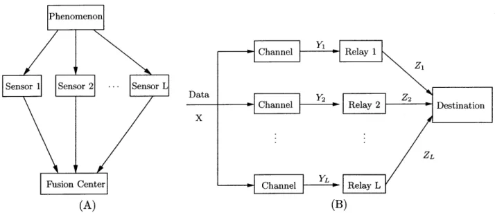
1-1 Sensors (A) and Relays (B) obtain noisy information and . . . . 18

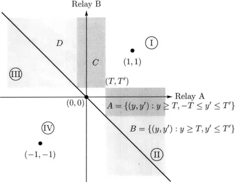
1-2 Arbitrary (T, T') relay decision threshold on the observation space . . . . 23

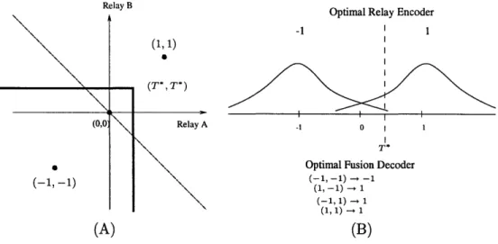
1-3 The optimal solution at T= (T*, T*) has the decision boundary . . . . 24

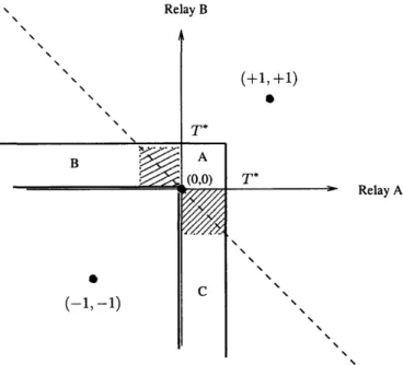
1-4 Tradeoffs in error by threshold at (T*, T*) compared to the obvious . . . . 25

2-1 The Error Curve. The parametric form . . . . 31

2-2 The error curve for the additive Gaussian noise channel. . . . 32

2-3 The Error Curve for the discrete case. . . . 35

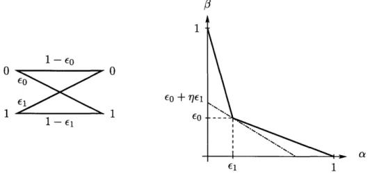
2-4 The Binary Asymmetric Channel (BAC) and its error curve. . . . 38

2-5 Possible values of V to assure convexity of the discrete error curve. . . . 40

2-6 An (N - 1) point error curve and its canonical channel representation. . . . 41

2-7 The error curve at the fusion point for two different BAC in parallel . . . 43

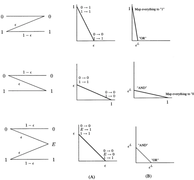
2-8 The error curve for the Z Channel and Binary Erasure Channel . . . . 45

3-1 The error curve for the equivalent channel . . . . 49

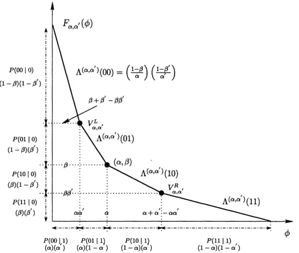
3-2 Fused error curve FQQ ( ) . . . . 51

3-3 Comparison of the fused error curves of a threshold test with that of a non-threshold test. . . . 52

(15)

3-5 For a given y and for a fixed a, the a' which minimizes error probability is the 1-tangent solution to F(#). . . . . 3-6 Fused curve for Relay A using threshold rule V, and Relay B using threshold

rule V' 57 . . . 5 8 3-7 3-8 3-9 3-10 3-11 3-12 3-13 3-14 3-15 3-16 3-17 3-18 3-19 3-20

3-21 The final fused error curve for the additive Gaussian noise channel. Whether V, or Va, or both are on F , (). . . . .

Fused left vertex point of independent randomized relay strategies Canonical DMC for a error curve with 2 vertex points. . . . . Partial structure of 2 point error curve. . . . . Convex Hull Matrix of allowed successive point . . . . Symmetric erasure-like relay channel and ML decoding at the fusion Symmetric erasure-like relay channel final fused curve . . . . The 3 stationary point solutions for the left vertex curve . . . . The iterative procedure stationary point solutions . . . . The fixed point solution . . . . The local minima solutions of the discrete error curve . . . . Discrete example of necessary conditions for optimality . . . . Functions of ratios of the Gaussian error function . . . . The chords do not intersect except at t = 0. . . . .

3-22 Construction of a relay error curve with an infinite number of stationary points. 3-23 Construction -infinite number of stationary points continued. . . . .

4-1 Equivalent performance of all 3 systems . . . . 4-2 Relay B as the fusion center. . . . . 4-3 The 2 x 3 system for the Additive Gaussian Noise Channel . . . .

. . . 59 . . . 67 . . . 69 . . . . 71 . . . 75 point. . . . 77 . . . 78 . . . 84 . . . 86 . . . 87 . . . 90 . . . 92 . . . 93 . . . 94 . . . 95 103 103 106 107 124

.

(16)

4-4 The 3 x 3 system for Additive Gaussian Noise Channel . . . 125 4-5 The 3 x 4 system for Additive Gaussian Noise Channel . . . 125 4-6 ML decoding for a symmetric relay error curve. . . . 130

(17)

Chapter 1 Introduction

1.1 Thesis Problem

There are many communication network situations where relays must each transmit a limited amount of information to a single destination which must fuse all the information together. For example, a large number of sensors could all be observing some source data which must be conveyed to a fusion center through limited communication channels. The measurements of the data are typically noisy, and the sensors usually are not able to communicate with each other since they are at physically different locations. Since each sensor is allowed to transmit very limited information to the destination, without knowing what the other sensors observe, it is not clear what information each sensor should send to the single destination. Another common example lies in a network of nodes where a number of nodes must act as relays but have no knowledge, except that from the source, about what the other relays receive. These relays all receive the same data, each corrupted by different noise, and must relay partial information about the data to a single destination. The destination fuses the information from these nodes to determine the original data. All relays and the destination have full knowledge of the code used at each relay and the decoding rule at the destination. It is assumed that no coding is permitted at the source. We assume, however, that all sensors know the statistics of the source, the noise statistics at all sensors, and the strategies of all sensors. Figure 1-1 depicts some typical scenarios.

(18)

Phenomenon

Sensor 11 Sensor 2 ... Sensor L:

Fusion Center

(A)

Data X Channel YL (L (B)

Figure 1-1: Sensors (A) and Relays (B) obtain noisy information and transmit/relay limited information to the Fusion Center/Destination

If the source X originates from a discrete distribution Qx, the problem involves distributed

detection. If the data originates from a continuous distribution FX, then the problem involves a distributed estimation problem. We restrict ourselves to distributed detection where the source is an independent identically distributed (i.i.d.) sequence generated from a fixed distribution Qx. In fact, we will usually restrict the source to be binary. The relay/sensor's observation space Y, which can be either discrete or continuous or both, will be quantized or coded and then sent to the destination or fusion point. The communication constraint between relay and fusion point determines the fineness of the relay quantization levels which we assume will be transmitted noiselessly. Otherwise, coding could be implemented on the quantized bits, and from the Coding Theorem, these bits could eventually be received by the fusion center with arbitrarily small probability of error.

Each channel can be modeled as a general discrete-time memoryless channel characterized by a conditional probability distribution for each input. One example of interest is the additive Gaussian noise channel where the noise has zero mean and unit variance. Another example of interest is the class of discrete memoryless channels (DMC) where the noise is described by a probability transition matrix P(Y

I

X).

Before studying the bigger problem of the distributed detection of an iid source sequence X' = {X}', we first study the one shot distributed detection problem of a single source symbol X. The one shot problem of detecting a single source symbol does have some advantages over encoding an entire sequence, such as no delay. However, it leaves less choice at the relays.

(19)

A relay can at most quantize the channel output, whereas encoding a long source sequence allows more sophisticated encoding at the relays, possibly resulting in better performance. For the one shot problem, given the relay encoders, it is straightforward to find the optimal fusion decoder. For certain special cases, given the fusion decoder, it may be possible to apply optimization techniques to finding the optimal relay encoders. In general, it is still difficult. For the distributed problems in this thesis, the simultaneous optimization of relay encoders and fusion decoder is necessary.

1.1.1 Special Case of Noiseless Channels

Much of the distributed nature of the system would be lost if the relays observed noiseless replicas of the data. Nevertheless, the noiseless observation case characterizes the asymptotic limit of very high signal to noise ratio (SNR). Suppose X is a discrete random variable and there are n relays, each of which can send at most one binary symbol. The fusion point receives n binary variables and decodes by mapping each binary n-tuple into some source symbol. Assume we have a minimum error probability criterion. Then the minimum error probability can be achieved if we could provide a distinct n-tuple from the set of relays to each of the most likely symbols and arbitrarily place each less likely uncoded symbol into the quantization bin of any coded symbol. Since each relay observes exactly the same thing, each can simply send one bit of the n-bit representation of the specified quantization code; the fusion center will then choose the most likely symbol in the specified quantization bin. For instance, Relay A can send the most significant bit, Relay B the next most significant bit, and so forth. The probability of error Pe is simply the sum of the probabilities of all the least probable symbols (the originally uncoded symbols) which are in a quantization bin with more than one symbol. For example, suppose the system consists of two relays, each allowed to send one bit. There are six data symbols with the following probabilities, Pr(A, B, C, D, E, F) = (n, , 3 , ) The destination receives a total of two bits. To minimize error probability, encode the four most probable symbols A - 0, B -- 1, C -- 2. D -> 3. Relay A sends the most significant bit with the mapping {A, B} -+ 0

and

{C,

D} -- 1, and Relay B sends the least significant bit with the mapping

{A,

C} -> 0 and

{B, D} -+ 1. The decoder decodes 00 -> A, 01 -> B, 10 - C, 11 -+ D with zero error. An

(20)

1.1.2 Special Case with Unlimited Communication from the Relays

The system also loses its distributed nature if there is no constraint on transmission rate from relay to destination. From the fusion center's perspective, the accuracy of the measurements increases as the allowed relay transmission rate increases. When each relay sends its full obser-vation Y, the scenario becomes a standard detection problem of estimating a random variable from a finite number of independent samples. Nevertheless, this case provides a lower bound on the error probability given a finite number of relays. Furthermore, if coding is allowed at the relays, this case also provides an upper bound on the maximum mutual information of the system in the asymptotic limit of increasing bit rate. The relay can use standard data compression on its output. The compression limit is H(Y) = - EZ log Pr(y). Therefore, as the relay output bits increase from 1 to H(Y), the system goes from a distributed to a centralized system.

1.1.3 Example of a Gaussian Channel with One Bit Relay Outputs.

We now look at the one shot distributed detection problem of a single source symbol X. To illustrate some aspects of this problem, let's look at the following simple, albeit important, example. Two relays, call them Relay A and Relay B, each observe a binary signal independently corrupted by 0-mean Gaussian noise. Each restricted to send at most one bit to the destination. The binary symbols are equally likely, the noises are independent of the input symbol and each other, and the receivers are not allowed to communicate nor have any side information about the other receiver's observation. The observations of relays A and B are, respectively, Y = X + N and Y' = X + N', x E {-1,+1}, Pr(X = +1) = Pr(X = -1) = 1/2, and N, N' are Gaussian AF(0, a2_{). Since only one bit relay transmission is allowed on a single source observation, it}

seems reasonable that the relay should just quantize the observation space. It is well known that that a threshold test on the likelihood ratio (LR) is the optimal strategy. For increased understanding, we will show via a different argument in Chapter 2, that a threshold tests are optimal. More generally, a quantization of the likelihood ratio of each relay's observation is optimal when they are allowed more symbols; this will be shown in Chapter 4. It is well known for the binary Gaussian detection problem that if each node is allowed to send its full observation to the decoder, the optimal decision boundary for Maximum Likelihood (ML) decoding is the line y = -y'. However, this is impossible to achieve since each relay is only allowed to send one bit to the destination. Upon receiving the two bits, the fusion center must decide whether

(21)

the original symbol is 1 or -1 with minimal error probability. This certainly appears like the classical detection problem of two independent samples of the data, so one would naturally think that the optimal solution would be for each relay to use a binary quantization with the origin separating the quantization regions. Letting Z E {-1, +1} and Z' E {-1, +1} denote the quantizer output of the relays, then Z= - 1 for Y < 0 and Z= + 1 for Y > 0. Likewise for

Z'. The fusion center maps (-1, -1) -> (-1) and (+1, +1) -- (+1), and arbitrarily decides the input for a (-1, +1) or (+1, -1) reception. This encoding/decoding scheme has the same error probability as if only one relay observation were used and the other relay ignored. The second relay does not help. For this specific quantizer, the reception of (-1, +1) or (+1, -1) carries no information and is a "don't care" map to either source symbol. To achieve better performance, it seems that (-1, +1) or (+1, -1) will need to carry some kind of information and having a second relay in the system should help. The importance of utilizing the (-1, +1) and (+1, -1) reception will become evident in the ensuing discussion.

Note that the map from the system input to the output of a relay takes the binary source input into a binary relay output. For the Gaussian problem above with a quantization at the origin, this map effectively produces a binary symmetric channel (BSC) with crossover probability Q

(1)

where Q (x) is the complementary distribution function' of the zero mean, unit variance

Gaussian density q(x) where

Q(x) = 1 e-2/2du q(x) = 1 e~x 2

/2 d

vl27 xV27 dx

Note that 1- Q (x) = Q (-x). Surprisingly, as we prove later in Chapter 3, the optimal solution

to this binary input additive Gaussian noise (AGN) 1-bit problem with equal priors and 2 relays is not a binary quantization separated at the origin, but rather a binary quantization separated at a point strictly away from the origin with each relay using the the same quantizer. These results were first shown in [IT94]. For one of the optimal solutions, both thresholds T and T' are set equal to T* where the relay outputs and T* are given by

( -1 for y < T* -1 for y' < T*

1 otherwise, ₁ _otherwise,

and

T =In[1 ."_i . (1.2)

'A slight variant of Q (x), used in the communication field, is the error function erf(x) = fo e- t2dt, which is also called the Gauss error function.

(22)

The decision rule at the fusion point is

-1

for(Z, Z') = (-1,

-1)

+1 otherwise

The resulting probability of error is

Pe= - 1

1 **Q (*+**

1)]

**[-Q (T*1)2)**

(1.4)

2 U0

From the symmetry of the signals, there exist two optimal solutions. The other solution simply uses the relay quantizer at -T* and a fusion point decision mapping of (+1, +1) -> +1 with

everything else mapped to -1. This is a totally symmetric problem with an asymmetric solution.

The asymmetry takes advantage of using (-1, +1) and (+1, -1) to carry information. It will soon be apparent how the gains in the asymmetric solution outweigh the costs. We now provide some intuition into the plausibility of this somewhat surprising result.

Let T and T' be arbitrary thresholds for Relays A and B, respectively. The encoding vector

T= (T, T') will split the observation region into 4 quadrants each corresponding to one of the

4 possible received vectors

Z

= (z, z') by the fusion point. Given any T, the optimal decoder

is easily calculated. In particular, for each quadrant, decode to the symbol which gives the minimum error probability. The following graphical argument shows how to determine the symbol for each region.

First assume that T + T' > 0 and observe the different decoding regions in figure 1-2. It is clear that when the fusion point receives (+1, +1) which is region I, it should map it to "+1" and region IV should be mapped to "-1". Region II can be divided into 2 regions, namely , A and B as shown in figure 1-2. The error probability is the same regardless of what region B is mapped to. Refer to these types of regions as "don't care" regions. Region A should be clearly mapped to "+1" since the likelihood of "+1" is greater than "-1" for every point in region A. Therefore, region II as a whole should be mapped to "+1". The same argument applies to region III. Region D={(y, y') : y < -T' and y' ; T'} is a "don't care" region and region

C={(y, y') : -T' < y < T and y' > T'} should be mapped to "+1." Thus, region III as a whole

should also be mapped to "+1." Now that the fusion decoder is fixed, we find the optimal T and T' that will minimize total error. Given the decoder map of (I,II,III,IV)=(1,+1,+1,-1), the optimal T equals (T*, T*), this will be derived in Chapter 3. By symmetry, if T + T' < 0, the optimal T equals (-T*, -T*). The optimal encoder and decoder map is unique and shown

(23)

in figure 1-3. Observe that when T + T' = 0, region A disappears and region II is just region B which is a "don't care" region. Likewise, region C disappears and region III is just region D which is also a "don't care" region. The regions can be optimally mapped into any of the following four choices {(+1, +1, +1, -1), (+1, -1, +1, -1), (+1, +1, -1, -1), (+1, -1, -1, -1)}.

The third and fourth choices are equivalent to decoding on the basis of the first relay alone or the second relay alone respectively. This is equal to the error probability of just a single relay observation as seen before.

The ML error probability for the case T = (T*, T*) is less than the ML error probability when T = (0, 0). We make two observations: First, the second relay is no longer redundant but useful in reducing error; and second, the "don't care" regions are now utilized. In other words, the (-1,

+1)

and (+1, -1) receptions are no longer "don't care" maps since they now carry information. Relay B D C(1, 1) (T, T') (0 Relay A (0 0 A= (y, y ,-T < y' < T'} B ={(y, y') : y T, y' < T'} (-1, -i)

Figure 1-2: Arbitrary (T, T') relay decision threshold on the observation space for T+T' > 0.

Fusion center receives 1 bit from each relay which specifies the 4 regions: I= {(y, y') : y >

T and y' > T'}, II={(y, y') : y > T and y' < T}, III= {(y, y') : y < T and y' > T}, IV= {(y, y') : y < T and y' < T'}. The "don't care" regions of whether a 1 or -1 is assigned to it are B and D. Region A and C should be assigned to "1."

Figure 1-4 shows the error trade-offs among the different schemes. First, compare the optimal solution at T = (T, T) with the suboptimal solution at T = (0,0). Since (-1, +1) and (+1, -1) are "Don't Care" decoding regions for T = (0,0), choose the same decoder for T = (0, 0) as for

(24)

T = (T*, T*) The small increase in error in region A is more than offset by an error decrease

in regions B and C. Note that if T is small, the increase in error probability in region A is proportional to T2, whereas the decrease in error probability in regions B and C is proportional

to T. Therefore, for small enough T, the solution at (T, T) has a smaller error probability than that at (0,0). In Chapter 3, we will show in detail why the two relays must use the same strategy. Solving for equation 1.2, we find there exists a unique point (T*, T*) which gives the optimal solution.

Relay B

Optimal Relay Encoder

-1 I

(1, 1)

(T*, T*)

(0,0 Relay A -1 0

T*

Optimal Fusion Decoder

(-1, -1) (--)- -1

(-1, 1) -+ 1

(1, 1) -* 1

(A) (B)

Figure 1-3: (A) The optimal solution at = (T*, T*) has the decision boundary shown by

the solid line. Points to the left and below the boundary map to "-1" and pints to the right and

above the boundary map to "1." (B) Corresponding relay encoder and optimal fusion point.

This simple example shows that these types of distributed problems are neither trivial nor obvious. The complete results for the additive Gaussian noise channel will be established in Chapter 3.

As the number of relays increases from two to L, the probability of error P decreases expo-nentially in L for any reasonable relay quantizer and decision mapping. Continuing with our toy problem, we increase the number of relays. The nontriviality of the problem is further apparent in the case of three relays for the AGN distributed system. Suppose the noise vari-ance is one and ML decoding is used at the fusion center. Then the error probabilities turn out to be within fractions of a percent of each other for the relay observation thresholds at

T=(T, T', T")=(0, 0, 0) with majority rule decoding and (T, T', T") = (0.2,0.2, -0.8) using the decoder {000, 010, 001} -+ 0, {100, 101, 011, 111} -+ _{1. The optimal result for the 3 relay case,} which uses a threshold T=(0, 0, 0) and majority rule decoding, will be proved with more insight in a future paper.

(25)

Relay B

(+1, +1)

T*

Relay A

(-1, -i)C

Figure 1-4: Tradeoffs in error by threshold at (T*, T*) compared to the obvious but subop-timal quantization at (T, T') = (0,0). Shaded regions are the "don't care" regions. Region

A = {0 < a,a' < T}, Region B = {a < -T* and 0 < a' < T*}, Region C = {0 < a < T and a' < -T}. The probability of error in Region A is Pe(A) - T2 and Region B and C are

Pe(B) = Pe(C) ~ Q (0) T. Thus, for small T the gain in decreased error (proportional to T)

from regions B and C is worth the cost in increased error (proportional to T2) in region A.

1.2 Previous Work and Background

The problem studied in this thesis is a sub-class of a classical problem in decentralized systems which was first posed by Tenney and Sandell in [TNS84I. The literature in the field is abundant since numerous people have worked on a number of variants of the distributed system problem. An excellent and thorough survey article [Tsi93] details the major contributions in this field of research. The book [Var97] and overview articles [VV97], [RB97] give a history and also discuss a number of variations in decentralized detection and coding.

Although more complicated networks have been addressed, parallel and serial topologies are generally considered. Almost across the board, the Bayesian and Neyman-Pearson approach is implemented. Conditional independence of sensor observations given the source is generally assumed, because the optimal solution is generally intractable otherwise. In [TA84] and [TA85], the authors proved that such problems are non-polynomial complete.

The asymptotic analysis of the system has already been well established by Tsitsikis in [Tsi88]. The complete asymptotic result and computational complexity as the number of relays tend to infinity is established. In general, any reasonable rule will drive the error probability down

(26)

exponentially in the number of relays. Tsitsikis further shows that for M hypothesis, the maximum number of distinct relay rules needed is M(M - 1)/2. Thus, for binary hypothesis, one single relay rule for each relay is sufficient for optimality as the number of relays tend to infinity.

Optimality of likelihood ratio tests at the relays and fusion point is well known. In our analysis, we will give a treatment and proof from a different viewpoint for added clarity. The problem with binary hypothesis and conditional independence assumptions (which is studied in this thesis) is the most studied in the literature. Various characteristics of the optimal solution for the binary detection problem and especially the specialized case of the additive Gaussian noise

channel has been given in [IT94], [QZ02], [WS01].

[Tsi93], [PA95], and [WW90] discuss randomized strategies. They recognized the non-convexity of the optimal non-randomized strategies, so dependent randomization was necessary for some cases. We will state precisely and supply the necessary conditions for the different types of randomization in our treatment.

[TB96] considered encoding long sequences of the source and looking at the rate-distortion function and [Ooh98] gave the complete solution to the specialized case for Gaussian sources. We by no means claim to give an exhaustive list of the field.

1.3 Outline of Thesis

Ad-hoc networks with a large numbers of nodes must use intermediate nodes to relay informa-tion between source and destinainforma-tion. This is a highly complicated problem. At the moment, there exists no structure to analyze the major issues in a fundamental way. This thesis attempts to understand and gain insight into a sub problem of this general problem of wireless networks. The thesis is organized as follows. Chapter 2 describes and characterizes the Neyman-Pearson error curve for arbitrary distributions and how it is utilized as a fundamental tool in analyzing the overall distributed detection and coding problem with relays. We prove some general results for the purely discrete case which will be used in later chapters. In Chapter 3, we study the joint optimization of relay encoder and fusion decoder. For the case of two relays, each sending a single bit to the fusion center, this will aid in the understanding of the optimal

(27)

solution and its structure. We provide a complete solution to the Gaussian case and also the optimal solution for arbitrary channels. Chapter 4 establishes the complete optimal solution and provides fundamental insights at the encoder and decoder for the case of 2 relays with non-binary outputs. Finally, chapter 5 concludes the thesis.

(28)

Chapter 2 The Error Curve

A significant part of this thesis deals with the detection of a binary digit through relays. Without relays, there are several approaches to the classical binary detection problem. In the maximum likelihood (ML) problem, we would like to minimize the overall error probability given equally likely inputs. More generally, in the maximum a posteriori (MAP) problem, we would like to minimize error probability for an arbitrary known input distribution. Even more generally, the minimum cost problem deals with minimizing overall cost given an arbitrary known input distribution and a cost function associated with each type of error. A final example of interest, known as the Neyman-Pearson problem , is to minimize the error probability of one type given a maximal tolerable error probability of the other type. In the classical problem without relays, the solutions to all these problems can be summarized by the error curve'. When relays are introduced into the system, we will find that the solution to all the above problems can be found from appropriately combining the error curves at the relays with an associated error curve at the fusion point.

This chapter will describe the Error Curve, its properties, and how it is used as a tool to both characterize the relays and the fusion process. The relay channels are described by error curves, and the final error curve at the fusion point is a function of the relay error curves.

(29)

2.1 Binary Detection and the Neyman-Pearson Problem

Binary detection for both discrete-alphabet and continuous-alphabet channels is characterized by the error curves. We start by reviewing binary detection without relays. We can view this in terms of a channel with binary input X and arbitrary output Y. Let the source a priori distribution be Pr(X=0)=po and Pr(X=1)=pi. Further, assume for now that fyx(YIO) and

fylx(Y|l) are densities. The discrete channel will be dealt with later in section 2.4. The likelihood ratio (LR) is defined for the set Y to be

A(Y) - fyx{Y 1} (2.1)

fylx{Yl

1}

For the values of y that are possible under X=1 but impossible under X=0, the likelihood ratio is A(Y) = 0. Likewise, for the values of y that are possible under X=0 but impossi-ble under X=1, A(Y) is infinite. We assume in this section that Pr (A(Y) rjX = 0) and Pr (A(Y) 1 X = 1) and Pr (A(Y) q) are continuous functions of ij. It follows that

Pr (A(Y) rIX = i) = 0 for all q and for i = 0, 1.

Define a test, t(Y) -+ {0, 1}, as a function which maps each output Y to 1 or 0. Define a randomized test over a finite set of tests {ti, t2, . .., tn} as a mapping

tg(Y) = ti(Y) with probability Oj (2.2)

where ?/ = (01, 42, .... , ./n) is the probability vector with which the tests {ti, t2, ... , tn} are

used.

Define a threshold test at 77 as a mapping

W1 if A(Y)< (2.3)

0 otherwise

A MAP test is any test which minimizes error probability for given a priori probabilities. The following lemma shows that the MAP test is a threshold test.

Lemma 2.1.1 A threshold test at q is a MAP test for a priori probabilities po and p1 where

=Pi

(30)

Proof: A MAP test decides X = 1 if Pr(X = 1 1 Y = y) > Pr(X = 0 1 Y = y) and decides X = 0 if Pr(X = 1 I Y = y) Pr(X = 0 1 Y = y). By Bayes Rule, this is the same as deciding X = 1 if A(Y) < q and X = 0 if A(Y) > T/. More compactly, for the continuous case,

x=O

A(Y) <> (2.4)

x=1

where by the assumption above, A(Y) has no point masses. D

Having cost functions associated with the different error probabilities is a more general problem but does not change the core of the problem. The optimal test for arbitrary cost is simply another threshold test. We show that changing the cost function and a priori probabilities in the system does not alter the fundamental problem. Let Cj be the cost of choosing hypothesis

i given hypothesis

j

has occurred. Let pi and po be the a priori probabilities, so 7 = P1. The PO

total cost becomes

C = p1P(011)Co1 +poP(1|O)C10 + poP(0|0)Co + p1P(1I1)Cn

= _{P(Ol)[piCo1 -poCool + P(1|0)[poCio -piCi] +poCoo +p1Cii}

= p'1P(0j1) + pP(1I0) +C' (2.5)

where p' = piCol - poCoo and pl = poCio - piC1 and C' = poCoo + piC1. The overall cost is minimized by a threshold test on the LR with threshold q, where

p' _ pico1 - PoCOO

P -P (2.6)

PO P0C10 - Pi 1 1

Thus, for any arbitrary cost, the problem is equivalent to solving the MAP problem with the modified a priori probabilities given in equation 2.6. If the MAP problem is solved for all apriori probabilities, it also solves the arbitrary cost problem. That is, the minimum cost problem is a trivial extension of the MAP problem. In what follows we will solve the arbitrary MAP problem.

For any given 1, let &(,q) = Pr(e I X = 1) and /(7) = Pr(e

I

X = 0) for the MAP test, i.e., the threshold test at i. Since Pr{A(Y)< 1 X=0} is continuous and increasing in 77, and

Pr{A(Y)r IX=1} is continuous and decreasing, we see that /(q) can be expressed as a function of &(q). Define the error curve by this pair of parametric functions of the threshold 'q, 0 < 77 < oo, called &(77) = Pr{A(Y) 77

I

X=1} and )(q) = Pr{A(Y)<7

I

X=0} both of which are

(31)

1-i(a)

tangent line slope of

,elO

-_p 11

11

Figure 2-1: The Error Curve. The parametric form of the error curve is described by

(&(77), iff) and the direct form of the curve by

~3

= /3(a). Each point (a, /3) on the error curve results from a threshold test with threshold value 77 = P1which is the magnitude of the slope of its point of tangency. The overall error probability is the value of the abscissa-intercept multiplied by a priori probability P0.

continuous functions of 77. That is, Pr{A(Y) = qj is zero for all q~. Then the ordinate and abscissa of the error curve are respectively,

&7)= PrfeIX=1} = Pr{A(Y)>?7IX=1} (2.7)

0q)= PrjejIX=O} = Pr{A(Y)<,qj X=O} = fl(o) (2.8)

As 77 increases, 03(,q) increases and

&(q)

decreases. The error curve is a graph plotting L(77) on the ordinate and &(77) on the abscissa as q goes from 0 to oo. An example of an error curve is shown in figure 2-1. The error curve is later shown to be convex. Note that &(77) is a monotonically decreasing function and f3() is a monotonically increasing function of q. Later we will treat the situation in which

&(77)

and ,3(77) are discontinuous. We call sections of the error curve which contain discontinuous &(77) and /3(7) the "discrete" part of the error curve

and treat it in a subsequent section. Define &(0)= limn'

0

&(77)

and &(oo)=

lim77,*0 &(,q)

and

03(0)= lim~l-+ 0

(-q)

and /3(oo)= lim- *(iO) When &(O) < 1, there is some event with non-zero

probability under X = _{1 and with probability zero under X}= 0. Likewise, when /3(Oo) < 1, there is some event with probability greater than zero under X = 0 and with probability zero under X = _{1. We call these types of curves erasure-like error curves.}

(32)

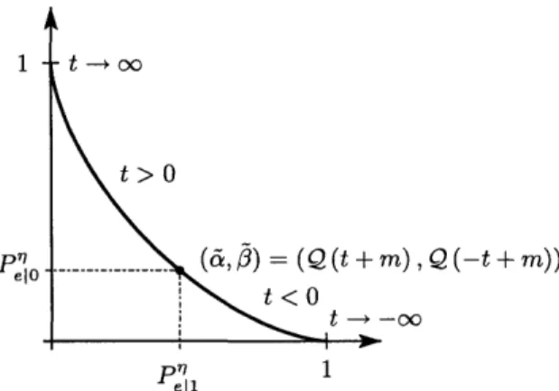
1 -t-+ oo 1t > 0 p _ _ (&,)=(Q(t+m),Q(-t+m)) t < 0 t -- oo

>I 0

eli

Figure 2-2: The error curve for the additive Gaussian noise channel. The parameters t and

m are normalized.

2.2 The Gaussian Error Curve

Let a relay observe a binary signal at signal level m or -m independently corrupted by Gaussian

noise, A(0,). SinceY=X+N, then Y=m+N if X =0 and Y= -m+N underX= 1.

We now describe the error curve for this additive Gaussian noise channel which we call the Gaussian error curve.

The Gaussian error curve is an example of an error curve which is strictly convex and everywhere differentiable. Thus, the function

&(r1)

is strictly decreasing and 3('r) strictly increasing . It is easier to represent the Gaussian error curve in parametric form, (a, 0) = (Q (Y9m), Q (Y2M)))

for m = 0 and a 0 and y E R. The LR is A(Y) = exp( 2 _{). Gaussian channels can be}

normalized and are completely characterized by one parameter, either the signal level m or variance a2. To see this, let t = then (a, ) =(Q(t

+

)

, Q (-t

+

E) for t E R. All that matters in the curve is the signal to noise ratio g. Thus, without loss of generality, we can assume a = 1 and let the mean m characterize the different Gaussian error curves. An example of a Gaussian error curve is illustrated in figure 2-2.

Furthermore, any single point (a*, 3*) on an error curve in the region a*+ 0* < 1 for a* > 0 and

0* > 0 completely specifies the Gaussian error curve. For any fixed point (a*, 0*), there exists

a unique t and m such that Q (t + m) = a* and Q (-t + m) = 0*. Thus, one point completely

determines the entire Gaussian error curve. From this point on, all Gaussian channels will be normalized with a = 1, mean m, and the error curve described parametrically with parameter t by (&(t), /(t)) = (Q (t + m) , Q (-t + m)), t

E

R and m 0 0. Additionally, observe that the LR is monotonic with the observation parameter y. Henceforth, for the rest of the thesis, whenever

(33)

the Gaussian case is discussed, rather than give solutions as thresholds on the likelihood ratio A(Y), we will represent solutions as observation thresholds of the parameter t for the normalized Gaussian error curve.

2.3 The q-tangent Line

We have seen that the error curve was generated from the MAP test over all threshold values. In this section, we will show that the value of the threshold q is the magnitude of the slope of the tangent line to its respective point on the error curve. This result is known but we give a new derivation and explanation. This simpler derivation will be useful in the distributed case later. Denote the line of slope -q through the point at (&(j), /(i)) as the q-tangent line as seen in figure 2-1. We now show that every 71-tangent line for an error curve lies on or below the entire error curve. We have seen that for given a priori probabilities po and pi, the threshold test at q = P minimizes error probability. Thus, for any arbitrary test x, it must be that

po/3(n) + pi&(,q)

poO(x) + pia(x)

(2.9)

0(q) +

O()

/(x) + ?la(x)

(2.10)

7(d(7)

-

a(x))

3(x)

-

(7)

(2.11)

Suppose a(x) < 5(n), then

/3(x) -/3(n) S< O 0(2.12)

- (n)

-

a(x)

The quantity on the right of 2.12 is the magnitude of the slope of the line connecting

(W(n),

3(7))

and (a(x), O(x)), so the point (a(x), 3(x)) must lie above the q-tangent line. For a(x) > a(nj), the inequality in 2.12 is reversed, again showing (a(x), 3(x)) lies above the n-tangent line. Thus, all the 77-tangent lines lie on or below the error curve. Furthermore, by the same argument, all the q-tangent lines lie below the point (&(,q), /3(,q)) for any test or randomized test. Finally, this argument also shows that all points of the error curve lie on the convex envelope2 of these tangent lines. Thus, every error curve is convex.

2

Define a convex combination of elements of a set X C R2 _{as a linear combination of the form}

A1X1 + A2 2 + - - + AnXn

for some n > 0, where each xi E X, each A, ; 0 and E Ai = 1. Define the convex hull, denoted co(X), to be

the smallest convex set which contains X. Define the convex envelope as the curve which is the lower boundary