Publisher’s version / Version de l'éditeur:
J. Syst. Software, 1999
READ THESE TERMS AND CONDITIONS CAREFULLY BEFORE USING THIS WEBSITE.
https://nrc-publications.canada.ca/eng/copyright
Vous avez des questions? Nous pouvons vous aider. Pour communiquer directement avec un auteur, consultez la première page de la revue dans laquelle son article a été publié afin de trouver ses coordonnées. Si vous n’arrivez pas à les repérer, communiquez avec nous à PublicationsArchive-ArchivesPublications@nrc-cnrc.gc.ca.
Questions? Contact the NRC Publications Archive team at
PublicationsArchive-ArchivesPublications@nrc-cnrc.gc.ca. If you wish to email the authors directly, please see the first page of the publication for their contact information.
NRC Publications Archive
Archives des publications du CNRC
This publication could be one of several versions: author’s original, accepted manuscript or the publisher’s version. / La version de cette publication peut être l’une des suivantes : la version prépublication de l’auteur, la version acceptée du manuscrit ou la version de l’éditeur.
Access and use of this website and the material on it are subject to the Terms and Conditions set forth at
The Prediction of Faulty Classes Using Object-Oriented Design Metrics
El-Emam, Khaled; Melo, W.
https://publications-cnrc.canada.ca/fra/droits
L’accès à ce site Web et l’utilisation de son contenu sont assujettis aux conditions présentées dans le site LISEZ CES CONDITIONS ATTENTIVEMENT AVANT D’UTILISER CE SITE WEB.
NRC Publications Record / Notice d'Archives des publications de CNRC:
https://nrc-publications.canada.ca/eng/view/object/?id=284d9d89-97be-4aaf-b706-aad56b4a24f3 https://publications-cnrc.canada.ca/fra/voir/objet/?id=284d9d89-97be-4aaf-b706-aad56b4a24f3National Research Council Canada Institute for Information Technology Conseil national de recherches Canada Institut de technologie de l'information
The Prediction of Faulty Classes Using
Object-Oriented Design Metrics *
El-Emam, K., Melo, W.
November 1999
* published as NRC/ERB-1064. November 1999. 24 pages. NRC 43609.
Copyright 1999 by
National Research Council of Canada
Permission is granted to quote short excerpts and to reproduce figures and tables from this report, provided that the source of such material is fully acknowledged.
National Research Council Canada Institute for Information Technology Conseil national de recherches Canada Institut de Technologie de l’information
The Prediction of Faulty
Classes Using Object-oriented
Design Metrics
Khaled El Emam and Walcelio Melo
November 1999
The Prediction of Faulty Classes Using
Object-Oriented Design Metrics
Khaled El Emam Walcelio Melo
National Research Council, Canada Institute for Information Technology
Building M-50, Montreal Road Ottawa, Ontario Canada K1A OR6 Khaled.El-Emam@iit.nrc.ca Oracle Brazil SCN Qd. 2 Bl. A Ed. Corporate, S. 604 70712-900 Brasilia, DF Brazil wmelo@br.oracle.com
Abstract
Contemporary evidence suggests that most field faults in software applications are found in a small percentage of the software’s components. This means that if these faulty software components can be detected early in the development project’s life cycle, mitigating actions can be taken, such as a redesign. For object-oriented applications, prediction models using design metrics can be used to identify faulty classes early on. In this paper we report on a study that used object-oriented design metrics to construct such prediction models. The study used data collected from one version of a commercial Java application for constructing a prediction model. The model was then validated on a subsequent release of the same application. Our results indicate that the prediction model has a high accuracy. Furthermore, we found that an export coupling metric had the strongest association with fault-proneness, indicating a structural feature that may be symptomatic of a class with a high probability of latent faults.
1 Introduction
Recent evidence indicates that most faults in software applications are found in only a few of a system’s components [50][31][40][55]. The early identification of these components allows an organization to take mitigating actions, such as focus defect detection activities on high risk components, for example optimally allocating testing resources [37], or redesign components that are likely to cause field failures. In the realm of object-oriented systems, one approach to identify faulty classes early in development is to construct prediction models using object-oriented design metrics. Such models are developed using historical data, and can then be applied for identifying potentially faulty-classes in future applications or future releases. The usage of design metrics allows the organization to take mitigating actions early and consequently avoid costly rework.
A considerable number of object-oriented metrics have been constructed in the past, for example, [6][10][19][48][47][18][15][38][66]. There have also been empirical studies validating various subsets of these metrics and constructing prediction models that utilize them, such as [2][18][1][10][12][14][47][20][36][54][66][6][16][7][53]. However, most of these studies did not focus exclusively on metrics that can be collected during the design stage.
In this paper we report on a study that was performed to construct a model to predict which classes in a future release of a commercial Java application will be faulty. In addition to identifying the faulty classes, the model can be applied to give an overall quality estimate (i.e., how many classes in the future release will likely have a fault in them). The model uses only object-oriented design metrics. Our empirical validation results indicate that the model has high accuracy in identifying which classes will be faulty and in predicting the overall quality level.
Furthermore, our results show that the most useful predictors of class fault-proneness are a metric measuring inheritance depth and a metric measuring export coupling, with export coupling having a dominating effect. These results are consistent with a previous study on a C++ telecommunications system, which found that export coupling was strongly associated with fault-proneness [28].
The paper is organized as follows. In the next section we provide an overview of the object-oriented metrics that we evaluate, and our hypotheses. In Section 3 we present our research method in detail, and in Section 4 the detailed results, their implications, and limitations. We conclude the paper in Section 5 with a summary and directions for future research.
2 Background
2.1 Metrics Studied
Our focus in this study are the two metrics sets defined by Chidamber and Kemerer [19] and Briand et al. [10]. In combination these constitute 24 metrics. Of these, only a subset can be collected during the design stage of a project. This subset includes inheritance and coupling metrics (and excludes cohesion and traditional complexity metrics).
At the design stage it is common to have defined the classes, the inheritance hierarchy showing the parent-child relationships amongst the classes, identified the methods and their parameters for each class, and the attributes within each class and their types. Detailed information that is commonly available within the definition of a method, for example, which methods from other classes are invoked, would not be available at design time. The cohesion metrics defined in these metrics suites were not collected for the same reason. This leaves us with a total of 10 design metrics that can be collected, two defined by Chidamber and Kemerer [19], and eight by Briand et al. [10].
The two Chidamber and Kemerer metrics are DIT and NOC. The Depth of Inheritance Tree [19] metric is defined as the length of the longest path from the class to the root in the inheritance hierarchy. It is stated that as one goes further down the class hierarchy the more complex a class becomes, and hence more fault-prone. The Number of Children inheritance metric [19] counts the number of classes which inherit from a particular class (i.e., the number of classes in the inheritance tree down from a class).
The Briand et al. coupling metrics are counts of interactions between classes [10]. The metrics distinguish between the relationship amongst classes (i.e., friendship, inheritance, or another type of relationship), different types of interactions, and the locus of impact of the interaction.
The acronyms for the metrics indicate what types of interactions are counted. We define below the acronyms and their meaning, and then summarize the design metrics.
• The first two letters indicate the relationship (A: coupling to ancestor classes; D: Descendents; and O: other, i.e., none of the above). Although the Briand et al. metrics suite covers it, friendship is not applicable in our case since the language used for the system we analyze is Java.
• The next two letters indicate the type of interaction between classes c and d (CA: there is a attribute interaction between classes c and d if c has an attribute of type d; and CM: there is a class-method interaction between classes c and d if class c has a class-method with a parameter of type class d). Method-method interactions are not available at design time. There is a method-method interaction between classes c and d if c invokes a method of d, or if a method of class d is passed as parameter to a method of class c.
• The last two letters indicate the locus of impact (IC: Import Coupling; and EC: Export Coupling). A class c exhibits import coupling if it is the using class (i.e., client in a client-server relationship), while it exhibits export coupling if is the used class (i.e., the server in a client-server relationship).
Ancestor-based coupling metrics that we considered were: ACAIC and ACMIC. The descendent-based coupling metrics that we considered were: DCAEC and DCMEC. The remaining coupling metrics cover the four combinations of type of interaction and locus of impact: OCAIC, OCAEC, OCMIC, and OCMEC.
2.2 Hypotheses
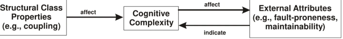
An articulation of a theoretical basis for developing quantitative models relating object-oriented metrics and external quality metrics has been provided in [12], and is summarized in Figure 1. This illustrates
that we hypothesise a relationship between the object-oriented metrics and fault-proneness due to the effect on cognitive complexity.
Structural Class Properties (e.g., coupling) Cognitive Complexity External Attributes (e.g., fault-proneness, maintainability) affect affect indicate
Figure 1: Theoretical basis for the development of object oriented product metrics.
There, it is hypothesized that the structural properties of a software component (such as its coupling) have an impact on its cognitive complexity. Cognitive complexity is defined as the mental burden of the individuals who have to deal with the component, for example, the developers, testers, inspectors, and maintainers. High cognitive complexity leads to a component exhibiting undesirable external qualities, such as increased fault-proneness and reduced maintainability.
Therefore, our general hypothesis is that the metrics that we validate, and that were described above, are positively associated with the fault-proneness of classes. This means that higher values on these metrics represent structural properties that increase the probability that a class will have a fault that causes a field failure.
3 Research Method
3.1 Data Source and Measurement
The system that was analyzed is a commercial Java application. The application implements a word processor that can either be used stand-alone or embedded as a component within other larger applications. The word processor provides support for formatted text at the word, paragraph, and document levels, allows the definition of groupings of formatting elements as styles, supports RTF and HTML external file formats, allows spell checking of a range of words on demand, supports images embedded within documents or pointed to through links, and can interact with external databases.
We consider two versions of this application: versions 0.5 and 0.6. Version 0.5 was fielded and feedback was obtained from its users. This feedback included reports of failures and change requests for future enhancements. To address these additional functionalities, version 0.6 involved an extensive redesign of the application, partially to avoid using an externally provided library which had critical limitations.
Version 0.5 had a total of 69 classes. The design metrics were collected from an especially developed static analysis tool. No Java inner classes were considered. For each class the design metrics were collected. Also, for each class it was known how many field failures were associated to a fault in that class. In total, 27 classes had faults. Version 0.6 had 42 classes. This version was also used in the field and based on failure reports a subsequent version of the application was released. For version 0.6, 24 of the classes had faults in them that could be traced to field failures.
In addition to the inheritance and coupling metrics, we collected two measures of size: the number of attributes defined in a class and the number of methods. The size measure that we use is the number of attributes defined in the class, denoted ATTS. This was defined as a size measure for object-oriented classes in the past [14]. Since our conclusions are not changed by this alternate size measure, we only consider the ATTS size measure in this paper.
In our analysis we used data from version 0.5 as a training data set, and data from version 0.6 as the test data set. As noted above, all faults were due to field failures occuring during actual usage. For each class we characterized it as either faulty or not faulty. A faulty class had at least one fault detected during field operation.
It has been argued that considering faults causing field failures is a more important question to address than faults found during testing [7]. In fact, it has been argued that it is the ultimate aim of quality
modeling to identify post-release fault-proneness [30]. In at least one study it was found that pre-release fault-proneness is not a good surrogate measure for post-release fault-proness, the reason posited being that pre-release fault-proneness is a function of testing effort [31].
3.2 Data Analysis Methods
Our data anslysis approach consists of four steps:1 1. Variable Selection
2. Calibration 3. Prediction
4. Quality Estimation
We describe the objectives of each of these steps below as well as the analysis techniques employed. 3.2.1 Variable Selection
During this step the objective is to identify the subset of the object-oriented metrics that are related to fault-proneness. These variables are then used as the basis for further modeling steps explained below. We select variables that are individually associated with fault-proneness and that are orthogonal to each other.
Variable selection is achieved by looking at the relationship between each metric and fault-proneness individually.2 The statistical modeling technique that we use is logistic regression (henceforth LR). This is explained in detail below as well as some diagnostics that are applied to check the stability of the resulting models.
Our approach accounts for the potential confounding effect of class size. This can be illustrated with reference to Figure 2. Path (a) is the main hypothesized relationship between an object-oriented metric and fault-proneness. We also see that class size (for example, measured in terms of number of attributes) is associated with the object-oriented metric (path (c)). Evidence supporting this for many contemporary object-oriented metrics is found in [14][12][18]. Also, class size is known to be associated with the incidence of faults in object-oriented systems, path (b), and is supported in [18][35][14]. The pattern of relationships shown in Figure 2 exemplifies a classical confounding effect [64][8]. This means that the relationship between the object-oriented metric and fault-proneness will be inflated due the effect of size. A recent study highlighted this potential confounding effect [27] and demonstrated it on the Chidamber and Kemerer metrics [19] and a subset of the Lorenz and Kidd [48] metrics. Specifically, this demonstration illustrated that without controlling for the confounding effect of class size one obtains results that are systematically optimistic. It is therefore necessary to control class size to get accurate results.
1
The research method presented here and that we use in our study is a refinement of the methodology used in a previous study [28].
2
We do not employ automatic selection procedures since they are known to be unstable. It is more common to use a forward selection technique rather than backward selection. The reason being that backward selection starts off with all of the variables and then eliminates variables incrementally. The number of observations is usually not large enough to justify construcing a model with all variables included. A Monte Carlo simulation of forward selection indicated that in the presence of collinearity amongst the independent variables, the proportion of ‘noise’ variables that are selected can reach as high as 74% [25]. It is clear that many object-oriented metrics are inter-correlated [12][14].
O-O
Metric
Fault-Proneness
Size
(a)
(b)
(c)
Figure 2: Path diagram illustrating the confounding effect of class size on the relationship between an object-oriented metric and fault-proneness.
3.2.1.1 Logistic Regression Model
Binary logistic regression is used to construct models when the dependent variable is binary, as in our case. The general form of an LR model is:
+ −
∑
+
=
= k i i ixe
1 01
1
β βπ
Eqn. 1where
π
is the probability of a class having a fault, and thex
i’s are the independent variables. Theβ
parameters are estimated through the maximization of a log-likelihood [39].As noted above, it is necessary to control for the confounding effect of class size. A measured confounding variable can be controlled through a regression adjustment [8][64]. A regression adjustment entails including the confounder as another independent variable in a regression model. Our logistic regression model is therefore:
( 0 11 2 2)
1
1
x xe
β β βπ
− + ++
=
Eqn. 2where
x
1 is the object-oriented metric being validated, andx
2 is size, measured as ATTS. We construct such a model for each object-oriented metric being validated.It should be noted that the object-oriented metric and the size confounding variable are not treated symmetrically in this model. Specifically, the size confounder (i.e., variable
x
2) should always be included in the model, irrespective of its statistical significance [8]. If inclusion of the size confounder does not affect the parameter estimate for the object-oriented metric (i.e., theβ
1 parameter of variable1
x
), then we still get a valid estimate of the impact of the metric on fault-proneness. The statistical significance of the parameter estimate for the object-oriented metric, however, is interpreted directly since this is how we test our hypothesis.In constructing our models, we follow previous literature in that we do not present results for interactions nor higher order terms (for example, see [27][2][6][10][11][12][14][66]). This is to some extent justifiable given that as yet there is no clear theoretical basis to assume any of the above.
The magnitude of an association can be expressed in terms of the change in odds ratio as the
x
1 variable (i.e., object-oriented metric) changes by one standard deviation, and is denoted by∆Ψ
, and is given by3:(
)
( )
σ
β1σ 1 1e
x
x
=
Ψ
+
Ψ
=
∆Ψ
Eqn. 3where
σ
is the standard deviation of thex
1 variable. 3.2.1.2 Diagnosing CollinearitySince we control for the size confounder through regression adjustment, careful attention should be paid to the detection and mitigation of potential collinearity. Strong collinearity can cause inflated standard errors for the estimated regression parameters.
Previous studies have shown that outliers can induce collinearities in regression models [52][61]. But also, it is known that collinearities may mask influential observations [3]. This has lead some authors to recommend addressing potential collinearity problems as a first step in the analysis [3], and this is the sequence that we follow.
Belsley et al. [3] propose the condition number as a collinearity diagnostic for the case of ordinary least squares regression4 First, let
߈
x be a vector of the parameter estimates, andX
is an
×
(
k
+
1
)
matrix of thex
ij raw data, withi
=
1
K
n
andj
=
1
K
k
, wheren
is the number of observations andk
is thenumber of independent variables. Here, the
X
matrix has a column of ones to account for the fact that the intercept is included in the models. The condition number can be obtained from the eigenvalues of theX
TX
matrix as follows:min max
µ
µ
η =
Eqn. 4where
µ
max≥
L
≥
µ
min are the eigenvalues. Based on a number of experiments, Belsley et al. suggestthat a condition number greater than 30 indicates mild to severe collinearity.
Belsley et al. emphasize that in the case where an intercept is included in the model, the independent variables should not be centered since this can mask the role of the constant in any near dependencies. Furthermore, the
X
matrix must be column equilibrated, that is, each column should be scaled for equal Euclidean length. Without this, the collinearity diagnostic produces arbitrary results. Column equilibration is achieved by scaling each column inX
,X
j, by its norm [4]:X
jX
j .This diagnostic has been extended specifically to the case of LR models [24][68] by capitalizing on the analogy between the independent variable cross-product matrix in least-squares regression to the information matrix in maximum likelihood estimation, and therefore it would certainly be parsimonious to use the latter.
The information matrix in the case of LR models is [39]:
3
In some instances the change in odds ratio is defined as:
(
)
( )
1 11
x
x
Ψ
+
Ψ
=
∆Ψ
. This gives the change in odds when the object-oriented metric increases by one unit. Since different metrics utilize different units, this approach precludes the comparison of the change in odds ratio value. By using an increment of one standard deviation rather than one unit, as we did, we can compare the relative magnitudes of the effects of different object-oriented metric since the same unit is used.4
Actually, they propose a number of diagnostic tools. However, for the purposes of our analysis with only two independent variables we will consider the condition number only.
( )
ß
X
V
X
I
ˆ
ˆ
=
Tˆ
Eqn. 5where
V
ˆ
is the diagonal matrix consisting ofπ
ˆ
ii(
1
−
π
ˆ
ii)
whereπ
ˆ
ii is the probability estimate from the LR model for observationi
. Note that the variance-covariance matrix of߈
is given byI
ˆ
−1( )
ß
ˆ
. One can then compute the eigenvalues from the information matrix after column equilibrating and compute the condition number as in Eqn. 4. The general approach for non-least-squares models is described by Belsley [5]. In this case, the same interpretive guidelines as for the traditoinal condition number are used [68].We therefore use this as the condition number in diagnosing collinearity in our models that include the size confounder, and will denote it as
η
LR. In principle, if severe collinearity is detected we would use logistic ridge regression to estimate the model parameters [60][61]. However, since we do not detect severe collinearity in our study, we will not describe the ridge regression procedure here.3.2.1.3 Hypothesis Testing
The next task in evaluating the LR model is to determine whether any of the regression parameters are different from zero, i.e., test
H
0:
β
1=
β
2=
L
=
β
k=
0
. This can be achieved by using the likelihoodratio
G
statistic [39]. One first determines the log-likelihood for the model with the constant term only, and denote thisl
0 for the ‘null’ model. Then the log-likelihood for the full model with thek
parameters is determined, and denote thisl
k. TheG
statistic is given by2
(
l
k−
l
0)
which has a2
χ
distribution withk
degrees of freedom.5If the likelihood ratio test is found to be significant at an
α
=
0
.
05
then we can proceed to test each of the individual parameters. This is done using a Wald statistic,( )
j j
e
s
β
β
ˆ
.
.
ˆ
, which follows a standard normal distribution. These tests were performed at a one-tailed alpha level of 0.05. We used one-tailed test since all of our alternative hypotheses are directional: there is a positive association between the metric and fault-proneness.
For each object-oriented metric, if the parameter of the object-oriented metric is statistically significant, then this metric is considered further. Statistical significance indicates that the metric is associated with fault-proneness. If the parameter for the object-oriented metric is not statistically significant then that metric is dropped from further consideration.
In previous studies another descriptive statistic has been used, namely an
R
2 statistic that is analogous to the multiple coefficient of determination in least-squares regression [14][12]. This is defined as0 0 2
l
l
l
R
=
−
kand may be interpreted as the proportion of uncertainty explained by the model. We use a corrected version of this suggested by Hosmer and Lemeshow [39]. It should be recalled that this descriptive statistic will in general have low values compared to what one is accustomed to in a least-squares regression. In our study we will use the corrected
R
2 statistic as an indicator of the quality of the LR model.3.2.1.4 Influence Analysis
Influence analysis is performed to identify influential observations (i.e., ones that have a large influence on the LR model). This can be achieved through deletion diagnostics. For a data set with
n
5
Note that we are not concerned with testing whether the intercept is zero or not since we do not draw substantive conclusions from the intercept. If we were, we would use the log-likelihood for the null model which assigns a probability of 0.5 to each response.
observations, estimated coefficients are recomputed
n
times, each time deleting exactly one of the observations from the model fitting process. Pergibon has defined the∆
β
diagnostic [56] to identify influential groups in logistic regression. The∆
β
diagnostic is a standardized distance between the parameter estimates when a group of observations with the samex
i values is included and when they are not included in the model.We use the
∆
β
diagnostic in our study to identify influential groups of observations. For groups that are deemed influential we investigate this to determine if we can identify substantive reasons for them being overly influential. In all cases in our study where a large∆
β
was detected, its removal, while affecting the estimated coefficients, did not alter our conclusions.3.2.1.5 Orthogonality Analysis
The above LR procedures will result in a subset of the metrics that have statistically significant parameters being retained. However, it is likely that some of these metrics are associated with each other. We use the robust Spearman correlation coefficient for investigating such associations [62].6 For metrics that are strongly associated with each other, we select only one of them for further consideration. The selected metric would be the one that has the largest change in odds ratio (i.e., the largest impact on fault-proneness).
The consequence of this step is that a small number of metrics remain that are both associated with fault-proneness and that are orthogonal.
3.2.2 Calibration
After identifying a subset of metrics that are associated with fault-proneness and that are orthogonal, we construct a multivariate model that combines all of these metrics. The construction of such a model follows the procedure described above, except that more variables will be incorporated.
The multivariate model can be practically applied in identifying which classes are likely to contain a fault (prediction step) and to estimate the overall fault content of a system (quality estimation step). The optimal operating point for the multivariate model is determined during calibration. This operating point maximizes the prediction accuracy. For calibration only the training data set is used (version 0.5).
It has been recommended that in studies where sample sizes are less than 100, as in our case, a leave-one-out approach provides reliable estimates of accuracy [69]. Therefore we use this approach during calibration.
3.2.2.1 Some Notation
It is common that prediction models using object-oriented metrics are cast as a binary classification problem. We first present some notation before discussing accuracy measures.
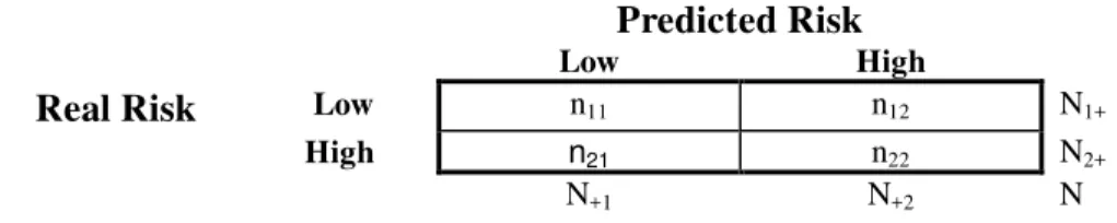
Table 1 shows the notation in obtained frequencies when a binary classifier is used to predict the class of unseen observations in a confusion matrix. We consider a class as being high risk if it has a fault and low risk if it does not have a fault.
Predicted Risk
Low High
Real Risk
Low n11 n12 N1+High n21 n22 N2+
N+1 N+2 N
Table 1: Notation for a confusion matrix.
6
We do not employ a multivariate technique such as a principal components analysis because usually a small number of metrics are retained and a simple correlation matrix makes clear the associations amongst them. If many metrics are retained, then it would be more appropriate to use a data reduction technique such as principal components analysis.
Such a confusion matrix also appears frequently in the medical sciences in the context of evaluating diagnostic tests (e.g., see [33]). Two important parameters have been defined on such a matrix that will be used for our exposition, namely sensitivity and specificity.7
The sensitivity of a binary classifier is defined as:
22 21 22
n
n
n
s
+
=
Eqn. 6This is the proportion of high risk classes that have been correctly classified as high risk classes. The specificity of a binary classifier is defined as:
12 11 11
n
n
n
f
+
=
Eqn. 7This is the proportion of low risk classes that have been correctly classified as low risk classes.
Ideally, both the sensitivity and specificity should be high. A low sensitivity means that there are many low risk classes that are classified as high risk. Therefore, the organization would be wasting resources reinspecting or focusing additional testing effort on these classes. A low specificity means that there are many high risk classes that are classified as low risk. Therefore, the organization would be passing high risk classes to subsequent phases or delivering them to the customer. In both cases the consequences may be expensive field failures or costly defect correction later in the life cycle.
3.2.2.2 Receiver Operating Characteristic (ROC) Curves
Recall that a logistic regression model makes predictions as a probability rather than a binary value (i.e., if we use a LR model to make a prediction, the predicted value is the probability of the occurrence of a fault). It is common to choose a cutoff value for this predicted probability. For instance, if the predicted probability is greater than 0.5 then the class is predicted to be high risk.
Previous studies have used a plethora of cutoff values to decide what is high risk or low risk, for example, 0.5 [13][12][2][51], 0.6 [12], 0.65 [12][14], 0.66 [11], 0.7 [14], and 0.75 [14]. In fact, and as noted by some authors [51], the choice of cutoff value is arbitrary, and one can obtain different results by selecting different cutoff values (see the example in [28]).
A general solution to the arbitrary thresholds problem mentioned above is Receiver Operating Characteristic (ROC) curves [49]. One selects many cutoff points, from 0 to 1 in our case, and calculates the sensitivity and specificity for each cutoff value, and plots sensitivity against 1-specificity as shown in Figure 3. Such a curve describes the compromises that can be made between sensitivity and specificity as the cutoff value is changed. One advantage of expressing the accuracy of our prediction model (or for that matter any diagnostic test) as an ROC curve is that it is independent of the cutoff value, and therefore no arbitrary decisions need be made as to where to cut off the predicted probability to decide that a class is high risk [73]. Furthermore, using an ROC curve, one can easily determine the optimal operating point, and hence obtain an optimal cutoff value for an LR model.
For our purposes, we can obtain a summary accuracy measure from an ROC curve by calculating the area under the curve using a trapezoidal rule [34]. The area under the ROC curve has an intuitive interpretation [34][65]: it is the estimated probability that a randomly selected class with a fault will be assigned a higher predicted probability by the logistic regression model than another randomly selected class without a fault. Therefore, an area under the curve of say 0.8 means that a randomly selected faulty class has an estimated probability larger than a randomly selected not faulty class 80% of the time.
7
The terms sensitivity and specificity were originally used by Yerushalmy [71] in the context of comparing the reading of X-rays, and have been used since.
When a model cannot distinguish between faulty and not faulty classes, the area will be equal to 0.5 (the ROC curve will coincide with the diagonal). When there is a perfect separation of the values of the two groups, the area under the ROC curve equals 1 (the ROC curve will reach the upper left corner of the plot).
Therefore, to compute the accuracy of a prediction logistic regression model, we use the area under the ROC curve, which provides a general and non-arbitrary measure of how well the probability predictions can rank the classes in terms of their fault-proneness.
3.2.2.3 Optimal Operating Point
The optimal operating point on the ROC curve is the point closest to the top-left corner. This gives the cutoff value that will provide the highest sensitivity and specificity. At the optimal cutoff one can also estimate the senstivity,
sˆ
, and specificity,fˆ
. These values are then used for quality estimation.Figure 3: Hypothetical example of an ROC curve. 3.2.3 Prediction
The calibrated model can be used to predict which classes have a fault in the test data set (version 0.6). The prediction results provide a relatistic assessment of how accurate this multivariate model will perform in actual projects.
The calibrated model with its optimal cutoff point already computed can be used to make binary risk predictions. Below we discuss different approaches that can be used for evaluating prediction accuracy. 3.2.3.1 Common Measures of Accuracy
Common measures of accuracy for binary classifiers that have been applied in software engineering are the proportion correct value, reported in for example [1][45][63] (also called correctness in [57][58]), completeness, for example [9][57] (which is equal to the senstivity), correctness which is the true positive
rate [9][14][12][13] (also called consistency in [57][58]), the Kappa coefficient [12][14], Type I and Type II misclassifications [41][42][44][43] (Type I misclassification rate is
1
−
f
, and the Type II misclassification rate is1
−
s
), and some authors report sensitivity and specificity directly [1].Proportion correct is an intuitively appealing measure of prediction performance since it is easy to interpret. With reference to Table 1, it is defined as:
N
n
n
11+
22 Eqn. 8However, in [29] it was shown that such an accuracy measure does not provide generalisable results. This can be illustrated through an example. Consider a classifier with a sensitivity of 0.9 and a specificity of 0.6, then the relationship between the prevalence of high risk classes in the data set and proportion correct is as depicted in Figure 4. Therefore, if we evaluate a classifier with a data set where say 50% of the classes are high risk then we would get a proportion correct value of 0.75. However, if we take the same classifier and apply it to another data set with say 10% of the classes are high risk, then the proportion correct accuracy is 0.63.8 Therefore, proportion correct accuracy is sensitive to the proportion of high risk classes (i.e., prevalence of high risk classes), which limits its generalisability. Similar demonstrations were made for other measures of accuracy, such as correctness and Kappa [29].
Prevalence P ro p o rti o n C o rr e c t 0.56 0.62 0.68 0.74 0.80 0.86 0.92 0.0 0.1 0.2 0.3 0.4 0.5 0.6 0.7 0.8 0.9 1.0
Figure 4: Relationship between prevalence (the proportion of high risk classes) and proportion correct for a classifier with sensitivity of 0.9 and specificity of 0.6.
Therefore, accuracy measures based on sensitivity and specificity are desirable (such as Type I and Type II misclassification rates). However, it is also desirable that a single accuracy measure be used, as opposed to two. The reason is best exemplified by the results in [43]. Here the authors were comparing nonparametric discriminant analysis with case-based reasoning classification. The Type I misclassification rate was lower for discriminant analysis, but the Type II misclassification rate was lower for the case-based reasoning classifier. From these results it is not clear which modeling technique is superior. Therefore, using multiple measures of accuracy can give confusing results that are difficult to interpret.
8
This is based on the assumption that sensitivity and specificity are stable. If this assumption is not invoked then there is no reason to believe that any results are generalisable, irrespective of the accuracy measure used.
3.2.3.2 The J Coefficient
The J coefficient of Youdon [72] was suggested in [29] as an appropriate measure of accuracy for binary classifiers in software engineering. This is defined as:
1
−
+
=
s
f
J
Eqn. 9This coefficient has a number of desirable properties. First, it is prevalence independent. For example, if our classifier has specificity and sensitivity equal to
f
=
0
.
9
ands
=
0
.
7
, then itsJ
value is 0.6 irrespective of prevalence. TheJ
coefficient can vary from minus one to plus one, with plus one being perfect accuracy and –1 being the worst accuracy. A guessing classifier (i.e., one that guesses High/Low risk with a probability of 0.5) would have aJ
value of 0. Therefore,J
values greater than zero indicate that the classifier is performing better than would be expected from a guessing classifier.We therefore use the J coefficient as a general indicator of the calibrated model’s prediction accuracy. The J value is computed by evaluating the calibrated model on the test data set (version 0.6).
3.2.4 Quality Estimation
The calibrated model can be used to estimate the overall quality of an object-oriented application. Here quality is defined as the proportion of classes that are faulty. A naïve estimate of the proportion of faulty classes is:
N
N
t
ˆ
=
+2 Eqn. 10However, as shown in [59], this will only be unbiased if both sensitivity and specificity are equal to 1. The corrected estimate of the proportion of faulty components is given by:
1
ˆ
ˆ
1
ˆ
ˆ
ˆ
−
+
−
+
=
f
s
f
t
p
Eqn. 11If both
sˆ
andfˆ
are equal to 1, thenp
ˆ
=
t
ˆ
. Since in practice this is unlikely to be the case, we should use Eqn. 11 to make the estimate.3.2.5 Summary
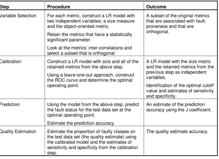
An overall summary of each of the four steps in our research method is provided in Table 2, including a description of the outputs.
Step Procedure Outcome Variable Selection For each metric, construct a LR model with
two independent variables: a size measure and the object-oriented metric.
Retain the metrics that have a statistically significant parameter.
Look at the metrics’ inter-correlations and select a subset that is orthogonal
A subset of the original metrics that are associated with fault-proneness and that are orthogonal.
Calibration Construct a LR model with size and all of the retained metrics from the above step. Using a leave-one-out approach, construct the ROC curve and determine the optimal operating point.
A LR model with the size metric and the retained metrics from the previous step as independent variables.
Identification of the optimal cutoff value and estimates of sensitivity and specificity.
Prediction Using the model from the above step, predict the fault status for the test data set at the optimal operating point.
Estimate the prediction accuracy.
An estimate of the prediction accuracy using the J coefficient.
Quality Estimation Estimate the proportion of faulty classes on the test data set (the quality estimate) using the calibrated model and the estimates of sensitivity and specificity from the calibration step.
The quality estimate accuracy.
Table 2: A summary of the steps in our research method.
4 Results
4.1 Descriptive Statistics
The descriptive statistics for the object-oriented metrics and the size metric for the train and test data sets are presented in Table 3 and Table 4 respectively. The tables show the mean, standard deviation, median, inter-quartile range (IQR), and the number of observations that are not equal to zero. In general, there are strong similarities between the two data sets. It is noticable that the OCAEC metric has a rather large standard deviation compared to the other metrics.
Variables ACAIC, ACMIC, DCAEC, and DCMEC have less than six observations that are non-zero on the training data set. Therefore, they were excluded from further analysis. This is the approach followed in previous studies [14][27].
Mean Median Std. Dev. IQR NOBS
≠
0 ACAIC .043 0 .205 0 3 ACMIC .173 0 .839 0 3 DCAEC 0 0 0 0 0 DCMEC 0 0 0 0 0 OCAIC 3.144 1 4.512 4 40 OCAEC 2.695 1 6.181 2 47 OCMIC 1.681 1 2.933 2 39 OCMEC 2.072 1 5.140 2 40 DIT 1.217 1 1.069 2 47 NOC .188 0 .624 0 7 ATTS 9.159 7 10.745 13 52Table 3: Descriptive statistics for all of the object-oriented metrics on the training data set (version 0.5).
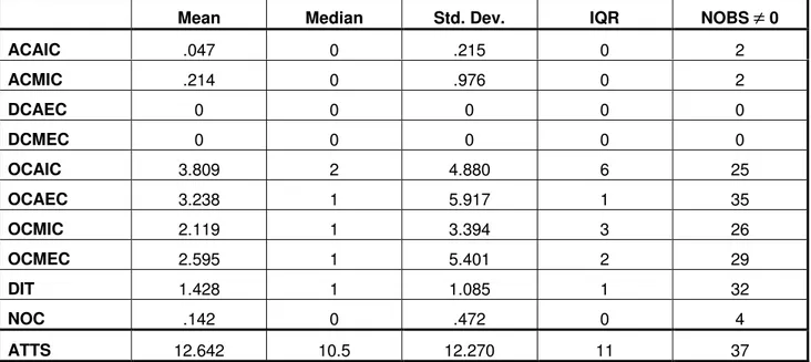
Mean Median Std. Dev. IQR NOBS
≠
0ACAIC .047 0 .215 0 2 ACMIC .214 0 .976 0 2 DCAEC 0 0 0 0 0 DCMEC 0 0 0 0 0 OCAIC 3.809 2 4.880 6 25 OCAEC 3.238 1 5.917 1 35 OCMIC 2.119 1 3.394 3 26 OCMEC 2.595 1 5.401 2 29 DIT 1.428 1 1.085 1 32 NOC .142 0 .472 0 4 ATTS 12.642 10.5 12.270 11 37
Table 4: Descriptive statistics for all of the object-oriented metrics on the test data set (version 0.6).
4.2 Variable Selection Results
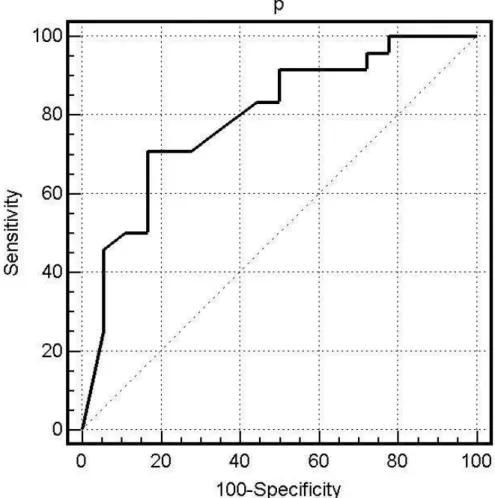
Table 5 contains the results of the LR models after controlling class size. The table only shows the parameters of the object-oriented metrics since this is what we draw conclusions from. This analysis was performed only on the training data set.
Metric G (p-value)
R2
LR
η
β2 Coefficient (s.e.) 1-sidedp-value
∆Ψ
OCAEC 42.45 (<0.0001) 0.49 5.80 2.5766 (0.6846) 0.0001 123 OCAIC 3.91 (0.1415) 0.0423 3.697 0.0541 (0.0801) 0.2498 1.276 OCMEC 29.57 (<0.0001) 0.33 3.64 1.2144 (0.3455) 0.0002 12.2 OCMIC 11.52 (0.0032) 0.124 2.61 0.3494 (0.1500) 0.0099 2.78 DIT 12.68 (0.0018) 0.137 3.869 0.7681 (0.2712) 0.0023 2.273 NOC 8.96 (0.0113) 0.099 2.239 -7.02 (25.07) 0.389 0.016 Table 5: Results of the validation, including the logistic regression parameters and diagnostics. Only four metrics out of the six had a significant association with fault-proneness: OCAEC, OCMEC, OCMIC, and DIT. The change in odds ratio for the OCAEC metric is quite large. Recall from Eqn. 3 that the change in odds ratio is a function of the standard deviation of the metric. OCAEC had a rather large standard deviation. This was due to a handful of observations that were extreme and hence inflated the variation. In general the standard deviation of this metric was sensitive to a minority of observations (i.e., removing them would have non-negligible impacts on the standard deviation). Therefore, the estimate of the change in odds ratio for OCAEC is quite unstable.Out of the remaining significant metrics, OCMEC had the largest change in odds ratio, indicating its strong impact on fault-proneness.
OCAEC OCMEC OCMIC
OCMEC 0.81 (<0.0001) OCMIC 0.50 (<0.0001) 0.71 (<0.0001) DIT 0.30 (0.0015) 0.15 (0.1067) 0.09 (0.3480) Table 6: Spearman correlations amongst the metrics that were found to be associated with
fault-proneness after controlling for size.
The Spearman correlations amongst the significant metrics are shown in Table 6. It is seen that all the coupling metrics are strongly associated with each other, with the strongest association between OCMEC and OCAEC. The DIT metric has a much weaker association with the coupling metrics.
We therefore select OCMEC and DIT for further investigation. We exclude OCAEC due to its unstable standard deviation (i.e., its usage would give us unstable results), 9 and exclude OCMIC since its change in odds ratio in Table 5 is smaller than that of OCMEC.
9
We also constructed a prediction model using the OCAEC metric instead of the OCMEC metric. The prediction accuracy was almost the same as that of the model using the OCMEC metric, but the model was, as expected, unstable.
4.3 Calibration
At this juncture we have identified two metrics that have value additional to class size, and that carry complementary information about the impact of class structure on fault-proneness. We now construct a multivariate LR model using these metrics.
G R2
LR
η
38.98; p<0.0001 0.4355 6.1737
Intercept ATTS OCMEC DIT
Coefficient -3.9735 0.0464 1.4719 1.0678
1-sided p-value 0.0001 0.1141 0.0004 0.0039
∆Ψ
1.603 20.746 3.156Table 7: Logistic regression results for the best model.
Table 7 shows the multivariate LR model incorporating the two metrics and size. It will be noted that the effect of the size measure, ATTS, is not significant. However, as noted earlier, we keep it in the model to ensure that the parameter estimates for the remaining variables are accurate.
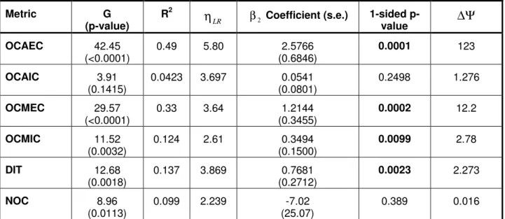
Figure 5: ROC curve for the calibration model. The area under the ROC is 0.87. The optimal operating point is at a cutoff value of 0.33, with a sensitivity of 0.81 and a specificity of 0.83.
The ROC curve for the model in Table 7 is shown in Figure 5. This curve was constructed using a leave-one-out approach. The area under this curve is 0.87, which is rather high in comparison to a previous study with object-oriented metrics [28]. The optimal cutoff value for this LR model is 0.33, which is quite different from the traditonally utilized cutoff values. The sensitivity and specificity of this model at the optimal operating point are estimated to be 0.81 and 0.83 respectively.
Now that we have calibrated the model (i.e., determined its optimal operating characteristics), it can be applied to predict which classes in the test data set (version 0.6) are going to be faulty.
4.4 Prediction
We used the model in Table 7 to predict which classes in the test data set will have a fault. Note that since we only use design metrics, this prediction can be performed at design time.
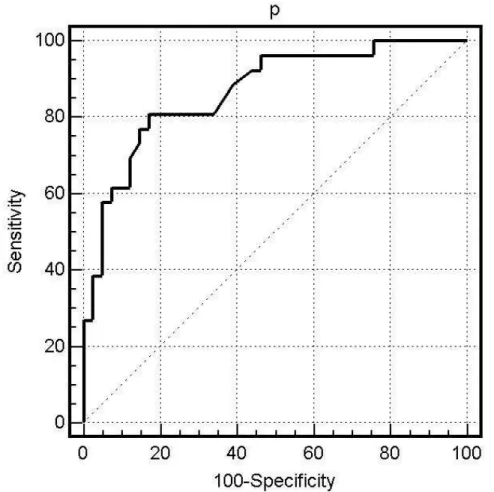
Figure 6: ROC curve for the test set. The area under the ROC curve is 0.78.
The ROC curve for the predictions on the test data set is shown in Figure 6. This curve has an area of 0.78, which is not far off from the leave-one-out estimate, and is very good. This indicates that this model would have a good prediction accuracy. The predictions at the optimal cutoff of 0.33 are shown in Table 8. The J value for this model is 0.49, which can be considered to be high.
Predicted Fault Status
Not faulty Faulty
Real Fault Status
Not faulty 14 4 18Faulty 7 17 24
21 21 42
Table 8: Prediction results in a confusion matrix. The J value for this is 0.49.
In practice, it is also informative to calculate the proportion correct accuracy for a prediction model when used in a particular context. The following equation formulates the relationship between sensitivity, specificity, prevalence of faulty classes, and proportion correct accuracy:
))
1
(
(
)
(
s
h
f
h
A
=
×
+
×
−
Eqn. 12where
A
is the proportion correct accuracy, andh
is the proportion of faulty classes. For example, if our prediction model is to be used on an actual project where only 10% of the classes are expected to have faults in them, then the proportion correct accuracy would be approximately 0.77.4.5 Quality Estimation
In version 0.6 of the system, the prevalence of classes that were faulty was 0.57, as can be seen in Table 8. The naïve estimate of the prevalence of faulty components is 0.50 (21/42). This is smaller than the actual prevalance. By using Eqn. 11 and the estimated sentsitivity and specificity, we can correct this estimate to obtain an estimate of 0.52. The corrected estimate is closer to the actual value.
In this particular example the LR model that we constructed was rather accurate on the test data set (version 0.6). Therefore, the naïve and corrected estimates were not far apart. However, it is clear that the corrected estimate is an improvement over the naïve estimate.
In general, a LR model constructed from the training data set can provide rather good quality estimates using the corrected formula. This is a considerable advantage as the LR model is usable at the design stage of a project.
4.6 Discussion of Results
Our results indicate that, in addition to a simple size metric, the OCMEC and DIT metrics can be useful indicators of fault-prone classes. They are both associated with fault-proneness after controlling for size, and when combined in a multivariate model can provide accurate predictions of which classes are likely to contain a fault. The added advantage of both of the above metrics is that they can all be collected at design time, allowing early management of software quality.
We have also added to the methodology initially presented in [27][28] by providing a correct technique for estimating the quality of an object-oriented system using design metrics. Our results indicate that such an estimate is rather accurate.
We found that an inheritance metric and an export coupling metric are both associated with fault-proneness. We discuss this finding and its implications on the design of object-oriented systems.
4.6.1 Relationship Between Inheritance Depth and Fault-Proneness
Previous studies suggest that depth of inheritance has an impact on the understandability of object-oriented applications, and hence would be expected to have a detrimental influence on fault-proneness. These are reviewed below.
It has been noted that “Inheritance gives rise to distributed class descriptions. That is, the complete description for a class C can only be assembled by examining C as well as each of C’s superclasses. Because different classes are described at different places in the source code of a program (often spread across several different files), there is no single place a programmer can turn to get a complete description of a class” [46]. While this argument is stated in terms of source code, it is not difficult to generalize it to design documents. Wilde et al. performed an interview-based study of two object-oriented
systems at Bellcore implemented in C++ and investigated a PC Smalltalk environment, all in different application domains study [70], indicated that to understand the behavior of a method one has to trace inheritance dependencies, which is considerably complicated due to dynamic binding. A similar point was made in [46] about the understandability of programs in languages that support dynamic binding, such as C++.
In a set of interviews with 13 experienced users of object-oriented programming, Daly et al. [21] noted that if the inheritance hierarchy is designed properly then the effect of distributing functionality over the inheritance hierarchy would not be detrimental to understanding. However, it has been argued that there exists increasing conceptual inconsistency as one travels down an inheritance hierarchy (i.e., deeper levels in the hierarchy are characterized by inconsistent extensions and/or specializations of super-classes) [26], therefore inheritance hierarchies may not be designed properly in practice. In one study Dvorak [26] found that subjects were more inconsistent in placing classes deeper in the inheritance hierarchy when compared to at higher levels in the hierarchy.
An experimental investigation found that making changes to a C++ program with inheritance consumed more effort than a program without inheritance, and the author attributed this to the subjects finding the inheritance program more difficult to understand based on responses to a questionnaire [17]. A contradictory result was found in [23], where the authors conducted a series of classroom experiments comparing the time to perform maintenance tasks on a ‘flat’ C++ program and a program with three levels of inheritance. This was premised on a survey of object-oriented practitioners showing 55% of respondents agreeing that inheritance depth is a factor when attempting to understand object-oriented software [21]. The result was a significant reduction in maintenance effort for the inheritance program. An internal replication by the same authors found the results to be in the same direction, albeit the p-value was larger. The second experiment in [23] found that C++ programs with 5 levels of inheritance took more time to maintain than those with no inheritance, although the effect was not statistically significant. The authors explain this by observing that searching/tracing through the bigger inheritance hierarchy takes longer. Two experiments that were partial replications of the Daly et al. experiments produced different conclusions [67]. In both experiments the subjects were given three equivalent Java programs to make changes to, and the maintenance time was measured. One of the Java programs was ‘flat’, one had an inheritance depth of 3, and one had an inheritance depth of 5. The results for the first experiment indicate that the programs with inheritance depth of 3 took longer to maintain than the ‘flat’ program, but the program with inheritance depth of 5 took as much time as the ‘flat’ program. The authors attribute this to the fact that the amount of changes required to complete the maintenance task for the deepest inheritance program was smaller. The results for a second task in the first experiment and the results of the second experiment indicate that it took longer to maintain the programs with inheritance. To explain this finding and its difference from the Daly et al. results, the authors showed that the “number of methods relevant for understanding” (which is the number of methods that have to be traced in order to perform the maintenance task) was strongly correlated with the maintenance time, and this value was much larger in their study compared with the Daly et al. programs. The authors conclude that inheritance depth per se is not the factor that affects understandability, but the number of methods that have to be traced. Further support for this argument can be found in a recent study of a telecommunications C++ system [28], whereby an ancestor based import coupling metric was found to be associated with fault-proneness, whereas depth of inheritance tree did not.
At design time it is not common that information is available to allow the tracing of method invocations up an inheritance hierarchy. For example, this information would not be available in class interface definitions. Therefore, even if evidence to this effect was found, it would not be actionable during the early design phase.
The fact that we found that the depth of inheritance tree to be associated with fault-proneness may be, according to previous literature reviewed above, due to two reasons:
• A badly designed inheritance hierarchy such that inherited classes are inconsistent with their superclasses; or
• The DIT metric is confounded with method invocations up the inheritance hierarchy, and in fact inheritance depth is not the cause of fault-proneness
Further focused studies are required to determine which of the above explanations are closer to reality. 4.6.2 Relationship between Export Coupling and Fault-Proneness
The effect of the export coupling metric in our results was much stronger than that of DIT. The export coupling metric that we selected considered class-method interactions, although we did find that it is strongly associated with class-attribute interactions as well. Therefore, a priori it seems reasonable to talk about export coupling in general since these two types of interactions tend to co-occur.
A previous study of a C++ telecommunications system [28] also noted that export coupling is associated with fault-proneness. While two studies do not make a trend, there appears to be some initial consistency in findings.
One can make two hypotheses about why export coupling is strongly associated with fault-proneness: • Classes that have a high export coupling are used more frequently than other classes. This
means that in operational systems their methods are invoked most frequently. Hence, even if all classes in a system have exactly the same number of faults in them, more faults will be discovered in those with high export coupling simply because they are exercised more. This hypothesis suggests that cognitive complexity is not the causal mechanism that would explain our findings.
• A client of a class d makes assumptions about d’s behavior. A class with more export coupling has more clients and therefore more assumptions are made about its behavior due to the existence of more clients. Since the union of these assumptions can be quite large, it is more likely that this class d will have a subtle fault that violates this large assumption space, compared to other classes with a smaller set of assumptions made about their behavior.
If either of the above hypotheses is true, it remains that they are not specific to object-oriented programs. The same phenomena can occur in traditional applications that followed structured design methodology. 4.6.3 Summary
Our results have highlighted certain structural properties of object-oriented systems that are problematic. While we cannot provide exact causal explanations for the findings that inheritance depth and export coupling are strongly associated with fault-proneness, we have posited some precise hypotheses that can be tested through further empirical enquiry.
4.7 Limitations
This study has a number of limitations which should be made clear in the interpretation of our results. These limitations are not unique to our study, but are characteristics of most of the product metrics validation literature. However, it is of value to repeat them here.
This study did not account for the severity of faults. A failure that is caused by a fault may lead to a whole network crash or to an inability to interpret an address with specific characters in it. These types of failures are not the same, the former being more serious. Lack of accounting of fault severity was one of the criticisms of the quality modeling literature in [32]. In general, unless the organization has a reliable data collection program in place where severity is assigned, it is difficult to retrospectively obtain this data. Therefore, the prediction models developed here can be used to identify classes that are prone to have faults that cause any type of failure.
It is also important to note that our conclusions are pertinent only to the fault-proneness dependent variable, albeit this seems to be one of the more popular dependent variables in validation studies. We do not make claims about the validity (or otherwise) of the studied object-oriented metrics when the external attributes of interest are, for example, maintainability (say measured as effort to make a change) or reliability (say measured as mean time between failures).
It is unwise to draw broad conclusions from the results of a single study. Our results indicate that two structural properties of object-oriented metrics are associated with fault-proneness. While these results provide guidance for future research on the impact of coupling and inheritance on fault-proneness, they should not be interpreted as the last word on the subject. Further validations with different industrial
systems are necessary so that we can accumulate knowledge and draw stronger conclusions, and explain the causal mechanisms that are operating.
5 Conclusions
In this paper we performed a validation of object-oriented design metrics on a commercial Java system. The objective of the validation was to determine which of these metrics were associated with fault-proneness, and hence can be used for predicting the classes that will be fault-prone and for estimating the overall quality of future systems. Our results indicate that an inheritance and an export coupling metric were strongly associated with fault-proneness. Furthermore, the prediction model that we constructed with these two metrics has good accuracy, and the method we employed for predicting the quality of a future system using design metrics also has a good accuracy.
While this is a single study, it does suggest that perhaps there are a small number of metrics that are strongly associated with fault-proneness, and that good prediction accuracy and quality estimation accuracy can be attained. This conclusion is encouraging from a practical standpoint, and hence urges further studies to corroborate (or otherwise) our findings and conclusions.
6 References
[1] M. Almeida, H. Lounis, and W. Melo: “An Investigation on the Use of Machine Learned Models for Estimating Correction Costs”. In Proceedings of the 20th International Conference on Software Engineering, pp. 473-476, 1998.
[2] V. Basili, L. Briand and W. Melo: “A Validation of Object-Oriented Design Metrics as Quality Indicators”. In IEEE Transactions on Software Engineering, 22(10):751-761, 1996.
[3] D. Belsley, E. Kuh, and R. Welsch: Regression Diagnostics: Identifying Influential Data and Sources of Collinearity. John Wiley and Sons, 1980.
[4] D. Belsley: “A Guide to Using the Collinearity Diagnostics”. In Computer Science in Economics and Management, 4:33-50, 1991.
[5] D. Belsley: Conditioning Diagnostics: Collinearity and Weak Data in Regression. John Wiley and Sons, 1991.
[6] S. Benlarbi and W. Melo: “Polymorphism Measures for Early Risk Prediction”. In Proceedings of the 21st International Conference on Software Engineering, pages 334-344, 1999.
[7] A. Binkley and S. Schach: “Validation of the Coupling Dependency Metric as a Predictor of Run-Time Fauilures and Maintenance Measures”. In Proceedings of the 20th International Conference on Software Engineering, pages 452-455, 1998.
[8] N. Breslow and N. Day: Statistical Methods in Cancer Research – Volume 1 – The Analysis of Case Control Studies, IARC, 1980.
[9] L. Briand, V. Basili, and C. Hetmanski: “Developing Interpretable Models with Optimized Set Reduction for Identifying High-Risk Software Components”. In IEEE Transactions on Software Engineering, 19(11):1028-1044, 1993.
[10] L. Briand, P. Devanbu, and W. Melo: “An Investigation into Coupling Measures for C++”. In Proceedings of the 19th International Conference on Software Engineering, 1997.
[11] L. Briand, J. Daly, V. Porter, and J. Wuest: “Predicting Fault-Prone Classes with Design Measures in Object Oriented Systems”. In Proceedings of the International Symposium on Software Reliability Engineering, pages 334-343, 1998.
[12] L. Briand, J. Wuest, S. Ikonomovski, and H. Lounis: “A Comprehensive Investigation of Quality Factors in Object-Oriented Designs: An Industrial Case Study”. International Software Engineering Research Network technical report ISERN-98-29, 1998.
[13] L. Briand, J. Wuest, S. Ikonomovski, and H. Lounis: “Investigating Quality Factors in Object-Oriented Designs: An Industrial Case Study”. In Proceedings of the International Conference on Software Engineering, 1999.
[14] L. Briand, J. Wuest, J. Daly, and V. Porter: “Exploring the Relationships Between Design Measures and Software Quality in Object Oriented Systems”. To appear in Journal of Systems and Software.