Constraining star formation rates and AGN feedback in high-z radio galaxies

(1)

HAL Id: tel-02475869

https://tel.archives-ouvertes.fr/tel-02475869

Submitted on 12 Feb 2020

HAL is a multi-disciplinary open access

archive for the deposit and dissemination of sci-entific research documents, whether they are pub-lished or not. The documents may come from teaching and research institutions in France or abroad, or from public or private research centers.

L’archive ouverte pluridisciplinaire HAL, est destinée au dépôt et à la diffusion de documents scientifiques de niveau recherche, publiés ou non, émanant des établissements d’enseignement et de recherche français ou étrangers, des laboratoires publics ou privés.

high-z radio galaxies

Theresa Maria Falkendal

To cite this version:

Theresa Maria Falkendal. Constraining star formation rates and AGN feedback in high-z ra-dio galaxies. Galactic Astrophysics [astro-ph.GA]. Sorbonne Université, 2018. English. �NNT : 2018SORUS248�. �tel-02475869�

(2)

SORBONNE UNIVERSITÉ

DOCTORATE THESIS

to obtain the title of Doctor of the Sorbonne Université in Astrophysics

Presented by

Theresa Maria F

ALKENDAL

Constraining star formation rates and

AGN feedback in high-z radio galaxies

Thesis Advisors: Matt L

EHNERT

, Carlos D

E

B

REUCK

, Joël V

ERNET prepared at Institut d’Astrophysique de Paris, CNRS (UMR 7095),

Sorbonne Université

Composition of the jury

Reviewers: Susanne AALTO - Chalmers University of Technology , Gothenburg, Sweden

Mark ALLEN - Strasbourg Astronomical Data Centre, Strasbourg, France

Advisor: Matt LEHNERT - IAP, Paris, France

Co-advisor: Carlos DEBREUCK - European Southern Observatory, Garching, Germany

Joël VERNET - European Southern Observatory, Garching, Germany

President: Frédéric DAIGNE - IAP, Paris, France

Examinators: David ELBAZ - CEA, Saclay, France

(3)

(4)

Abstract

The evolution of galaxies is something that is still not well understood. Events such as, galaxy mergers, gas accretion from the cosmic web, metal enrichment and galactic nuclear activity affects further galaxy growth and shapes the evolution of galaxies. The cosmic star formation rate den-sity peaks between 1 < z < 3. It is therefore important to investigate the high-z Universe and the mechanisms which triggers or quenches star-formation. The impact of active galactic nuclei (AGN) have been hypothesized through cosmological simulations to be crucial in quenching the star-formation rate, but the mechanism behind this is not understood in detail. This is where high-z observations of AGN feedback in galaxies are important, to put tight constants on the Physics at play. In this thesis I investigate the effects of in-situ AGN feedback by studying high-z radio galaxies (HzRGs). These objects provide unique laboratories to study the interplay between AGN, gas, stars and feedback processes.

Millimeter Astronomy has recently seen major advances due to the development of the ALMA telescope, which opens up the possibility to probe the cold Universe at resolutions and depths never seen before. During my thesis I utilize the capabilities of ALMA by probing dust emission in a sample of 25 HzRGs at 1< z <5.2. I combine these new observations with previous data to constrain the star formation rates by multi-wavelength spectral energy distribution (SED) fitting. The ALMA data reveal that the morphology of the _∼1 mm continuum emission can be compli-cated, with contributions from several thermal dust emission components and/or synchrotron emission. The sensitivity and spatial resolution of the ALMA data required me to develop a SED fitting routine that can combine multi-resolution photometric observations and simultaneously fit the SED of galaxies detected in multiple components. We disentangle the far-infrared continuum emission of these 25 galaxies into dust heated by star-formation and AGN, as well as from contri-butions from synchrotron emission. This leads to new much more constraining estimates of the star formation rates of HzRGs, on average 7 times lower compared to estimates based only on Her-schel. The low star-formation rates in these objects compared to the main-sequence of star forming galaxies show that HzRGs seem to be on their way of being quenched. We might therefore be observing the effect of the AGN suppressing the growth of the host galaxy.

In the second part of the thesis, I explore the possibilities of constraining the gas Physics of the host galaxy and the halo gas by combining MUSE and ALMA data cubes. MUSE is also a relatively new instrument with impressive capabilities to probe ionized gas at rest-frame ultraviolet wave-lengths in the high-z Universe. I show extended ionized gas around the HzRG 4C 19.71, where the most remarkable feature is the most distant extension of the CIVgas beyond the radio lobes.

This gas is quiescent and coincide with a molecular gas reservoir detected with ALMA in [CI]. These observations show the power of multi-wavelength observations, but also the limitations of putting constraints when only a few emission lines are available.

These studies show how new more detailed observations help constrain important properties of HzRGs. These objects are being revealed to be more complicated than previously thought, showing large differences one source to another and new data sometimes raise more questions than they answer. But these type of studies have the potential of increasing our understanding of the physically mechanisms for AGN feedback and the interplay between the AGN, host galaxy and the halo gas.

(5)

(6)

Résumé

L’évolution des galaxies n’est toujours pas bien compris. Des évènements tel que des fusions de galaxies, l’accrétion à partir de la toile cosmique, l’enrichissement des métaux et l’activité des noy-aux affecte la croissance supplémentaire et façonne l’évolution des galaxies. Le tnoy-aux de formation d’étoiles culmine entre 1 < z < 3. Il est donc important d’étudier l’Univers à grand z et les méchanismes qui déclenchent ou étouffent la formation d’étoiles. Les simulations cosmologiques prévoient que l’influence des noyaux actifs de galaxies est primordial dans l’étouffement du taux de formation d’étoiles, mais les détails de ce méchanisme restent à élucider. C’est ici que les ob-servations de la rétroaction à grand z sont primordiaux pour contraindre la Physique. Dans cette thèse, j’étudie les effets de la rétroaction in-situ en utilisant les radiogalaxies distantes. Ces objets fournissent des laboratoires uniques pour étudier l’interaction des noyaux actifs des galaxies, le gaz, les étoiles et les processsus de rétroaction.

L’astronomie (sub)millimétrique a fortement progressé grâce à l’arrivée du télescope ALMA, qui permet les études de l’Univers froid à des résolutions et profondeurs jamais atteints aupara-vant. Dans cette thèse, j’utilise les capacités d’ALMA en sondant l’émission des poussières dans un échantillon de 25 radiogalaxies à 1 < z< 5.2. Je combine ces nouvelles observations avec des données précédentes afin de contraindre les taux de formation d’étoiles en utilisant l’ajustement des distributions d’énergie spectrales (SED) multi-longeur d’ondes. Les données ALMA montrent que la morphologie de l’émission continu à∼1 mm peut être compliquée, avec des contributions de plusieurs componsantes d’émission thermique de poussières et/ou du synchrotron. La sensi-bilité et la résolution spatiale d’ALMA nécessitaient que je développe une routine d’ajustement du SED pouvant combiner des observations photométriques multi-résolutions et ajuster simul-tanément les SED des galaxies détectés dans multiples composantes. Nous démèlons l’émission du continu infrarouge lointain de ces 25 galaxies en poussières chauffées par formation d’étoiles et noyau actif de galaxie, ainsi que des contributions de l’émission synchrotron. Ceci mène à des nouvaux taux de formation d’étoiles beaucoup plus contraignantes dans ces radiogalaxies, en moyenne 7 fois plus faibles comparés aux estimations basées seulement sur les données Her-schel sondant le pic de l’émission thermique. Les faibles taux de formation d’étoiles comparés à la séquence principale des galaxies formant des étoiles montrent que les radiogalaxies sont en route d’être étouffées. On pourrait donc observer l’effet du noyau actif supprimant la croissance de la galaxie hôte.

Dans la deuxième partie de la thèse, j’explore les possibilités de contraindre la Physique des gaz de la galaxie hôte en combinant les cubes de données MUSE et ALMA. MUSE est aussi un nou-vel instrument avec des capacités impressionnantes pour sonder le gaz ionisé aux longeurs d’onde ultra-violets au repos dans l’Univers lointain. J’étudie le gaz ionisé dans la radiogalaxie 4C 19.71, où la caractéristique la plus remarquable est l’extension la plus éloignée du gaz CIVau delà des

lobes radio. Ces observations montrent la puissance des observations multi-longeur d’onde, mais aussi les limitations à mettre des contraintes quand seulement quelques raies d’émission sont disponibles.

Ces études montrent comment des observations plus détaillées peuvent contraindre les pro-priétés des radiogalaxies. Ces objets deviennent de plus en plus complexes à mesure que de nou-velles données deviennent disponibles. Les galaxies montrent égallement de grandes différences en les regardant source par source, et les nouvelles données soulèvent parfois plus de questions qu’elles ne répondent. Mais ce genre d’études ont le potentiel d’améliorer notre compréhension

(7)

des méchanismes physiques de la rétroaction et l’interaction entre la galaxie hôte et le milieu cir-cumgalactique.

(8)

List of Figures

1.1 Black hole accretion rate compared to star-formation rate history. Left: average BH accretion

rate compared to the SFRD by Hopkins & Beacom (2006) and Fardal et al. (2007) scaled by

the factor M•/Mstar = 8×10−4. Figure reprint from review by Heckman & Best (2014)

(originally published by Shankar et al. 2009). Right: Black hole accretion rate scaled by a factor of 5000 and compared to the cosmic SFR reported by Hopkins (2004) and Bouwens et al. (2012). Reprinted from Kormendy & Ho (2013) (updated from Aird et al. 2010). . . 2 1.2 The M_•–MK,bulgeand M•– σecorrelation for ellipitcal galaxies and classical bulges (classified

as being indistinguishable from elliptical galaxies, except that they are embedded in disks), with fitted slopes and gray shaded region showing the 1σ of the fits. Figure reprinted from review by (Kormendy & Ho 2013) . . . 3

1.3 Schematic representation of the difference between the observed galaxy luminosity function

(blue line) and the theoretically predicted one (red line). By invoking supernova and AGN feedback in semi-analytic models, it is possible to closer reproduce observed galaxy proper-ties. Figure reprinted from (Silk & Mamon 2012). . . 4

1.4 The main sequences of star forming galaxies with the four main classes of galaxies based

on their location in the star-formation rate (SFR) vs stellar mass (M?) plane. Credit: Harry

Ferguson . . . 13 1.5 Two color composite images of Barnard 68, a molecular cloud located at a distance of∼130 pc,

showing the effect of dust attenuation and reddening of stellar radiation at different wave-lengths. Left: image composed of three optical filters, B-band 0.44 µm (blue), V-band 0.55 µm (green) and I-band 0.90 µm (red). Right: in false color B-band 0.44 µm (blue), I-band 0.85 µm

(green) and near-IR Ks-band 2.16 µm (red). Credit: ESO/press release eso0102. . . . 15

1.6 The extinction curve of the Milky Way for different degrees of reddening, RV=2.5, 3.1, 4.0 and

5.5. Apart from the rise towards the ultraviolet, the extinction increases around the 2175 Å bump. Image reprinted from (Li & Mann 2012). . . 16

1.7 Two different views of M31, Andromeda, in visible light originating from stars and in

in-frared light (24 µm, in false color) from dust emission. In the optical, the bulge dominates. The spiral arms are more distinct in the infrared image. This illustrates the advantages of multi-wavelength astronomy. Credit: NASA/JPL-Caltech/Univ. of Ariz., visible: NOAO, infrared: Spitzer. . . 17

1.8 Modeled spectral energy distribution of dust compared to COBE data (Arendt et al. 1998) of

observed infrared emission per H nucleus from dust heated by the average starlight back-ground in the Milky Way. Left: dust model consisting of large silicates (Si), amorphous carbon (aC), small silicates (sSi), graphite (gr) and PAHs. Reprinted from (Siebenmorgen et al. 2014). Right: model SED composition are from silicate (Si, dotted line), grains (Gra, dashed line)

and PAHs (dashed-dotted line). Reprinted from (Popescu et al. 2011) . . . 18

1.9 The unification model of AGNs. The galaxy properties depend mainly on the viewing

an-gle, whether or not jets are present and the power of the radio emission. Reprinted from (Beckmann & Shrader 2012). . . 24

1.10 Generic synchrotron spectrum from a galaxy hosting an AGN. Credit: SAO . . . 25

1.11 Overview of the main components needed to crate the emission from normal galaxies in the

wavelength range UV to FIR. Reprinted from (Conroy 2013) . . . 31

1.12 Inspection of the ALMA high site in 2016 by the author and CDB. . . 34

1.13 Atmospheric transmission as a function of wavelength, given for three different column

den-sities of percipitable water vapour (PWV). Credit: ALMA European arc . . . 35

(13)

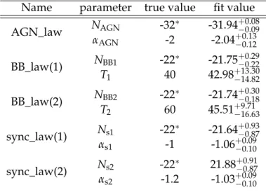
2.2 MC-Chains for each parameter for the given number of steps for example #1. Note the con-vergence reached roughly after step #100 . . . 50

2.3 Triangle diagram for example #1. The diagonal represents the marginalised probability

dis-tribution. The vertical dashed line correspond to the 10%, 25%, 50%, 75% and 90% percentiles of the distribution. The 50% percentile parameter along the 25% and 75% percentile values are reported in Table 2.6. The other diagram represents the 2D projection of the parame-ter space on the corresponding parameparame-ters on the abscissa and ordinate axes. The contours

represents the density distribution at 75%, 50% and 25% of the maximum parameter value . 51

2.4 SEDs for example #1. Note that the uncertainties are plotted but are smaller than the

data-points, diamonds being detections. left: best fit plot. The plain black line is the sum of the different components in each arrangement. right “spaghetti” plot. The best fit here is re-ported as the black plain line for each component (defined in the .dat file). The shaded area is the sum of each model representation after convergence (values of the parameters at each step of each walker). . . 51

2.5 Scheme of the combination of observations at different wavelengths from the data file to

illustrate the considered example. The circle sizes are relative to the resolution of the ob-servation but not to scale (see Fig. 2.6). Note that Herschel, LABOCA, one ALMA, one VLA and ATCA observations are not resolving the different components. From bigger to small circles: Herschel, ATCA, VLA, LABOCA, ALMA, double circles are VLA and ALMA(closer to center), and in the center Spitzer. . . 53

2.6 Images generated from the information contained data file assuming a Gaussian point spread

function, all images scaled to the same coordinates. Frequency is decreasing toward the right and the top. Note that no sources are detected in spire_350, spire_500 and laboca_870 images, while VLA_X and VLA_C present two components. North is top and East is left on all images. 54

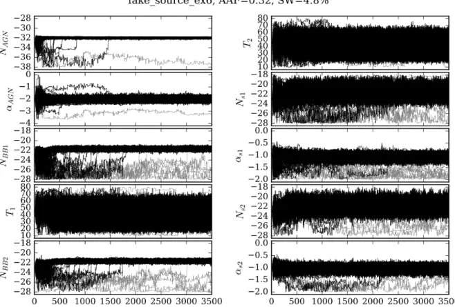
2.7 MC-Chains for each parameter for the given number of steps for example 2. Note the

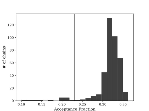
con-vergence reached roughly after 1000 steps. The grey lines are the “stuck” walkers, excluded from further analysis (see § 2.3.2 and Fig. 2.8). . . 55 2.8 Histogram of the acceptance fraction of the 400 chains. Note the cut at 0.23, chains under this

values are reported in grey in Fig. 2.7, which are the “stuck walkers” (see text § 2.3.2). . . 56

2.9 Triangle diagram for example #2. The diagonal represents the marginalised probability

dis-tribution. The vertical dashed line correspond to the 10%, 25%, 50%, 75% and 90% percentiles of the distribution. The 50% percentile parameter along the 25% and 75% percentile values are reported in Table 2.7.The other diagrams represent the 2D projection of the parameter space on the corresponding parameters on the abscissa and ordinate axes. The contours

rep-resents the 75%, 50% and 25% of the maximum parameter value. . . 57

2.10 Total SED for each arrangement of data and models plot in a single figure. Coloured lines refer to the different models and the black lines are the total of all components in each ar-rangement. This figure is reported for pedagogic purposes only as, given the increasing complexity of the system, a split SED is much clearer to disentangle the various contribution of the components to the data (see Fig. 2.11). . . 58 2.11 SEDs for example #2, split into subplots to illustrate each arrangement. Note that the

un-certainties are plotted but are smaller than the datapoints. Diamonds are detections while downward triangle are upper limits. top: best fit plot. The plain black line is the sum of the different components in each arrangement. bottom “spaghetti” plot. The best fit here is re-ported as the black plain line for each component (defined in the .dat file). The colours refer

to each model component, consistently between each subplot. . . 59

2.12 MC-Chains for example #3. Note the convergence after roughly 100 steps. Top: detections only(a). Bottom: detections and upper limits(b). . . 60 2.13 Triangle diagram for example #3. Top: detections only (a). Bottom: detections and upper limits

(b). The diagonal represents the marginalised probability distribution. The vertical dashed line correspond to the 10%, 25%, 50%, 75% and 90% percentiles of the distribution. The 50% percentile parameter along the 25% and 75% percentile values are reported in Table 2.8. The other diagram represents the 2D projection of the parameter space on the corresponding parameters on the abscissa and ordinate axes. The contours represents the 75%, 50% and 25% of the maximum parameter value . . . 61

(14)

2.14 SEDs for example #3. Top: detections only(a). Bottom: detections and upper limits(b). Left: Best fit plot. Right: Spaghetti plot. The diamonds are the detections and the triangles are the

1σ upper limits. Note that the fitting can converge above the upper limits to a certain extent. 62

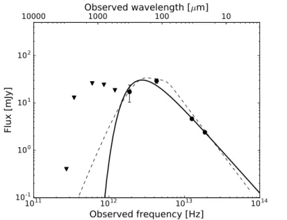
3.1 The best fit of the SED of 4C 23.56 when assuming that the AGN is solely responsible for the

mid-infrared emission and allowing λcutto be an additional free parameter. The black solid

line shows the best fit with λcut=33+3₋₃ µm. The dashed line is the best fit AGN model used

in Drouart et al. (2014) which itself is the average AGN used in the DecompIR SED fitting

code (Mullaney et al. 2011). See Table A.23 for details about the photometric data. . . 72

3.2 A comparison of the integrated IR AGN and SF luminosities computed in this paper

com-pared to the results of Drouart et al. (2014). (top) A comparison between the infrared luminos-ity of the AGN and (bottom) a comparison between the infrared luminosluminos-ity of the starburst or star forming component. In both panels, the dashed line is the one-to-one relationship between luminosities. . . 79

3.3 Model comparison between the SF and AGN models of this paper and Drouart et al. (2014)

for galaxies MRC 0350-279 (top left), MRC 0251-273 (top right), MRC 0156-252 (bottom left) and MRC 0211-256 (bottom right). In each plot, the black solid lines represent the synchrotron emission, dotted lines indicate the FIR thermal emission due to star-formation, and dash-dotted indicates the best-fit MIR emission due to the AGN as determined from the best fits to the photometry for each galaxy. The red lines with the same styles represent the same components as fitted in Drouart et al. A synchrotron power-law was not fit in the analysis of Drouart et al. . . 80 3.4 The estimated AGN luminosity, LIR_AGN, versus the SF luminosity, LIR_SF. The dashed black line

indicates the values where LIR_AGN= LIR_SF, while the dotted black line indicates parallel growth of the stellar mass and black hole mass, ˙Macc

BH=0.002×SFR. Filled black circles are galaxies

detected with ALMA and with constrained SF and AGN luminosity estimates. Purple arrows are sources with upper limit in the ALMA band. The upper limits of LIR_SFare approximated by scaling a modified black body to the 3-σ upper limit estimated assuming β=2.5 and T=50 K. We note that we assumed β=2.5 for all of our fits and 50 K is approximately the medium temperature of our best fits (Table 3.5). Black arrows indicate galaxies which are detected in ALMA but where the observed ALMA flux(es) are consistent with an extrapolation of the lower frequency synchrotron emission implying little or no contribution from thermal dust emission. We indicate with bars in the lower right corner of the plot, how the upper limits of the LIR_SFwould shift if one of the fixed parameters, β or T, are changed with respect to our assumed values of β=2.5 and T=50 K. . . 83

3.5 Relationship between the SFR and stellar mass for different redshift bins. The colored shaded

regions shows the MS of (Santini et al. 2017) for each respective redshift bins with a 0.3 dex scatter around the MS. The gray shaded regions shows the MS with a 0.3 dex scatter from Schreiber et al. (2015), with a turnover at higher stellar masses. Our stellar masses have been scaled from a Kroupa to a Salpeter IMF to be consistent with the IMF used to make the MS in this comparison. In the highest redshift bin, 3< z< 4, two sources, TN J1338+1942 and TNJ0924-2201, have been added to the right most panel despite having redshifts outside of the range used to construct the MS (z=4.110 and 5.195 respectively). Given the redshift de-pendence on the normalization of the MS, these galaxies may lie relatively lower in compar-ison with the mean relation of a MS derived using galaxies over a more appropriate, higher redshift range (see Fig. 3.6). . . 87 3.6 Specific star formation rate, sSFR (Gyr−1), as a function of redshift. The black filled circles,

black arrows and purple arrows represent the radio galaxies of our sample that are detected, detected but with unconstrained SF component and undetected with ALMA, respectively. The diamonds indicate sources which have both upper limits on the stellar mass and the SFR. The shaded region shows the galaxy main sequence (adapted from Schreiber et al. 2015) for M∗=1011.33M. We only indicate the redshift range 0.5<z<4 in the shaded region as z=4

is the redshift limit of the objects studied in Schreiber et al.. We do not extrapolate to higher redshifts (Stark et al. 2013). . . 89

(15)

3.7 Comparison of our results in the LSF–LAGN plane to other studies. LIRAGNfor our sample is

scaled by a factor 6 to estimate the bolometric luminosity. Black circles indicate sources de-tected with ALMA. Black downward pointing arrows indicate sources dede-tected in ALMA where the sub-mm flux is consistent with being dominated by synchrotron emission. Pur-ple downward pointing arrows indicate sources not detected with ALMA. The X-ray se-lected sources from Netzer et al. (2016) detected with Herschel over the redshift range z=2-3.5 are indicated with green squares; the large open green square is the SFR of the undetected sources which were stacked to estimate their median SFR. Blue triangles indicate X-ray se-lected sources from Stanley et al. (2015) over the redshift range, 1.8<z<2.1. The red line is the fit from Rosario et al. (2012) to the mean relation for AGNs over the redshift range 1.5<z<2.5 scaled up by a factor of 2 (see Netzer et al. 2016, for details). We indicate when the luminosity due to star formation equals that of the AGN with a black solid line. . . 91 3.8 Star formation rate, SFR in M.yr−1, versus the projected physical size of the radio

emis-sion in kpc, calculated using the largest angular size (LAS) of the radio emisemis-sion at 1.4 GHz (De Breuck et al. 2010). Black filled circles are detections, black arrows detections but with

unconstrained SF component and purple arrows non-detections (see text for details). . . 93

4.1 Six views around 4C19.71 from previous publications. Top left: smoothed 0.5–8 keV Chandra

images Smail et al. (2012); top center:; K-band 2.0–2.45 µm (Armus et al. 1998); top left: IRAC 3.6 µm (Seymour et al. 2007); bottom left: MIPS 24 µm (De Breuck et al. 2010); bottom center: ALMA band 3 continuum of 94.6–98.4 GHz and 106.5–110.3 GHz (Falkendal et al. 2018); bot-tom right: VLA band C 4.8 GHz (Pentericci et al. 2000). Pink plus indicate the center of the host galaxy determined from the peak of the thermal dust emission of the ALMA band 3 continuum image. Green crosses indicated the hot sport of the two radio lobes. The blue filled circles show the location of four foreground galaxies around 4C19.71. For details about coordinates and redshifts of the sources in the field see table A.26. The unmarked continuum sources in the different images are stars. . . 100 4.2 Five narrow band images of 4C19.71. Top left: Lyα (λobs=5581.64–5584.14 Å); top center: CIV

1548.2 Å (λobs=7100.39–7102.89 Å); top right: HeII(λobs=7525.39–7535.39 Å); bottom left CIII]

(λobs=8739.14–8756.64 Å); bottom center: [C I](1–0) ( 107.21–107.27 GHz) from the continuum

subtracted cube. bottom right: 13_{CO(4–3) (96.007–96.067 GHz) from continuum subtracted}

cube. MUSE moment-0 maps are smoothed with a Gaussian filter of size 7×7 pixels. Pink

contours is overlaid [C I](1–0) line emission (levels at 2.5σ, 3σ and 3.5σ, σ=29 mJy). Green contours is overlaid VLA band C (levels at 3σ,√2×3σ, 3√2×3σ and 5√2×3σ, σ=45 µm.) 102

4.3 Greyscale images of CIVemission in 4C19.71. The regions bound by red lines are positions

of the spectra extracted from the MUSE cube, determined from the CIVnarrow band image.

The regions bound by cyan lines indicate the position of the extracted [CI] spectra from

the ALMA cube, defined from the [CI] mom-0 map to maximize the S/N. The north [CI]

detection is unresolved and extracted by a beam size. The extracted spectra are shown in figure 4.4. . . 104 4.4 Extracted spectra of three different regions, as seen in Fig. 4.3. Left to right: North, Core and

South. Top to bottom: Lyα, CIV, and HeIIfrom the MUSE cube and [CI] from the ALMA

cube. The x-axes of the spectra are velocity relative to the systemic redshift, measured from the [CI] line at the core, zero indicated in dashed black. The y-axes are flux densities. Lower

panels of Lyα, CIV, and HeII: skyline spectra. Yellow shaded regions: wavelength channels

strongly affected by the skyline subtraction. Red lines: fitted line profiles, for details see Sec. 4.3.1 and Sec. 4.3.2. Dashed blue, green, cyan and magenta lines: theoretical HeIIlines if width and centering were the same as the CIVline and the flux ratio HeII/CIVwas 0.5, 1, 2, and 3, respectively. Solid cyan curve: spectrum of the non-detected13CO(4–3) line at the core. 106 4.5 The line ratios of [CI]/CIV as a function of CIV/HeII. The colored points represent the

models as indicated in the legend. The ionization parameter of each of the group of points in the figure are indicated in the appropriate regions (decreasing from -1 to -4 from left to right). For each of the isochoric models, the density of the gas increases upwards from log nH=0 to 3.

We also show a set of isobaric models for 3 pressures, P/k=2, 3 and 4. The red box show the estimated location from our observations. We note that the box shown greatly exaggerates that uncertainty in [CI]/CIVand show the range of plausible values for CIV/HeIIand not the uncertainties in the estimate. . . 109

(16)

A.1 SED of MRC 0037-258. Black solid line represents the best fit total model, green dashed line is synchrotron power-law of the radio core, dotted line indicates the AGN contribution. The colored data points indicate the data which have sub-arcsec resolution and black points indicate data of low spatial resolution. Green pentagons represent the fluxes from the radio core and the blue diamond indicates ALMA band 6 detection. Filled black circles indicate detections (>3σ) and downward pointing triangles indicate the 3σ upper limits (Table A.1). . 124 A.2 Panel A: continuum map of ALMA band 6 in grayscale with overplotted VLA C contours (the

levels are 3σ,√2×3σ, 3√2×3σ and 5√2×3σ (σ = 46 µJy)). The blue diamond indicates

the ALMA detection and is the same marker used in Fig. A.1. The green contours show the portion of the VLA data that is used in the SED fit, the red contours are excluded in the fit. Panel B: MIPS 24 µm continuum map with the same VLA C contours overplotted. . . 124 A.3 MRC 0037-258 Corner plot of the free parameters. . . 125 A.4 SED of MRC 0114-211. Black solid line shows best fit total model, green and purple dashed

lines are the western and eastern synchrotron lobes, respectively. The black dash-dotted line is one black body component associated to one of the ALMA band 6 detections. Black dotted line indicates the AGN component. The colored points indicate data with sub-arcsec resolu-tion and black ones indicate the data with low spatial resoluresolu-tion. Green pentagons indicate the western radio lobe, purple hexagons indicate the eastern radio lobe, the blue diamond indicates one of the ALMA band 6 detection, and the magenta square is the second ALMA detection. Filled black circles indicate detections (>3σ) and downward pointing triangles the 3σ upper limits (Table A.2). . . 127 A.5 Panel A: continuum map of ALMA band 6 with VLA C contours overlaid (levels are as

Fig. A.2; σ = 71 µJy). The blue and pink markers indicate the two different components

detected with ALMA and correspond to the same data points as Fig. A.4. The purple and green contours show the two components of the VLA data and correspond to the markers of the same colors as in the SED fit. Panel B: MIPS 24 µm continuum map with VLA 4.7 GHz contours overlaid. Note that the scale of the MIPS image is 5 times larger than the image displayed in panel A. . . 127 A.6 MRC 0114-211 Corner plot of the free parameters. . . 128 A.7 SED of TN J0121+1320. Black solid line shows the best fit total emission model, black dashed

line represents the synchrotron emission and the black dash-dotted lines represents the black body emission. The colored data point indicate the data with sub-arcsec resolution and black ones indicated data of low spatial resolution. The blue diamond indicates the ALMA band 3 detection. Filled black circles indicate detections (>3σ) and downward pointing triangles the 3σ upper limits (Table A.3). . . 130 A.8 Panel A: continuum map of ALMA band 3 with overlaid VLA C contours (levels are as Fig.

A.2, σ=70 µJy) Panel B: MIPS 16 µm continuum map. . . 130 A.9 TN J0121+1320 Corner plot of the free parameters. . . 131 A.10 SED of MRC 0152-209. Black solid line shows best fit total model, black dashed line

repre-sents the total synchrotron emission. The magenta and blue dashed-dotted line represent the two black bodies of the northern and southern ALMA 6 detections, respectively. Black dot-ted line indicates the AGN component. The colored data points indicate data with sub-arcsec resolution and black ones indicate data of lower spatial resolution. The magenta square and blue diamond indicates the ALMA band 6 detection of the northern and southern compo-nents, respectively. Filled black circles indicate detections (>3σ) and downward pointing triangles the 3σ upper limits (Table A.4). . . 133 A.11 Panel A: continuum map of ALMA band 6 with overlaid VLA C contours (levels are as Fig.

A.2, σ=56 µJy). The blue and pink markers show the two ALMA detections and correspond

the same markers used in Fig. A.10. Panel B: MIPS 24 µm continuum map and please note that the scale of the MIPS image is 5 times larger. . . 133 A.12 MRC 0152-209 Corner plot of the free parameters. . . 134

(17)

A.13 The SED of MRC 0156-252. Black solid line shows the best fit total model, green and purple dashed line represents the northern lobe and synchrotron emission from the core, respec-tively. Black dotted line indicates the AGN component. The colored points are data which have sub-arcsec resolution and black ones indicate data of lower resolution. Green pentagons represent the fluxes of the radio core, purple hexagons are the fluxes of the northern radio lobe, the blue diamond indicates the ALMA band 6 detection which coincides with the radio core and the magenta square is the second ALMA detection of the northern radio lobe. Filled black circles indicate detections (>3σ) and downward pointing triangles 3σ upper limits (Ta-ble A.5). . . 136 A.14 Panel A: continuum map of ALMA band 6 with overlaid VLA C contours (levels are as Fig.

A.2, σ=96 µJy). The blue and pink markers show the two ALMA detections and correspond

to the same markers used for the SED in Fig A.13. The core and northern radio lobes are color coded in the same colors as the flux markers in Fig. A.10, the flux of the southern lobe (red radio contours) was not used in the SED fit. Panel B: PACS 70 µm continuum map with radio contours overlaid. . . 136 A.15 MRC 0156-252 Corner plot of the free parameters. . . 137 A.16 SED of TN J0205+2242. Black solid line shows best fit total model, green and purple dashed

line is the north and south synchrotron, respectively. The colored data points are sub-arcsec resolution data and black ones indicated data of low resolution. The blue and purple down-ward pointing triangles indicates the ALMA band 3 upper limits at the location of the two radio lobes, where the blue triangle is the upper limit of the host galaxy and the north syn-chrotron component. Filled black circles indicate detections (>3σ) and downward pointing triangles the 3σ upper limits (Table A.6). . . 139 A.17 Panel A: continuum map of ALMA band 3, overlaid VLA C contours (levels are as Fig. A.2,

σ = 85 µJy). Blue and purple markers indicate the two different upper limits with ALMA

and correspond to the same data points as Fig. A.16. The green and purple show the two components of the VLA data and correspond to the markers of the same colors as in the SED fit. Panel B: IRS 16 µm continuum map. . . 139 A.18 TN J0205+2242 Corner plot of the free parameters. . . 140 A.19 SED of MRC 0211-256. Black solid line shows best fit total model, dashed line is total

syn-chrotron, dash-dotted line is the black body component and the dotted line indicates the AGN component. The colored data point is sub-arcsec resolution data and black ones indi-cated data of low resolution. Blue diamond indicates ALMA band 6 detection. Filled black circles indicate detections (>3σ) and downward pointing triangles the 3σ upper limits (Ta-ble A.7). . . 142 A.20 Panel A: continuum map of ALMA band 6 with overlaid VLA C contours (levels are as Fig.

A.2, σ= 86 µJy). The blue diamond indicates the ALMA detection and is the same marker

used in Fig. A.19. The green contours show the portion of the VLA data that is used in the SED fit. Panel B: MIPS 24 µm continuum map. . . 142 A.21 MRC 0211-256 Corner plot of the free parameters. . . 143 A.22 SED of TXS 0211-122. Black solid line shows best fit total model, green dashed line is total

synchrotron, black dash-dotted line is the black body component, black dotted line indicates the AGN component. The colored data points are sub-arcsec resolution data and black ones indicate data of low resolution. Green pentagons are the radio core and the blue diamond indicates ALMA band 6 detection. Filled black circles indicate detections (>3σ) and down-ward pointing triangles the 3σ upper limits (Table A.8). The open diamond shows available ATCA data but only plotted as a reference and was not used in the SED fit. . . 145 A.23 Panel A: continuum map of ALMA band 6 with overlaid VLA C contours (levels are as Fig.

A.2, σ= 53 µJy). The blue diamond indicates the ALMA detection and is the same marker

used in Fig. A.22. The green contours show the portion of the VLA data that is used in the SED fit, the red contours are excluded in the fit. Panel B: MIPS 24 µm continuum map. . . 145 A.24 TXS 0211-122 Corner plot of the free parameters. . . 146

(18)

A.25 SED of MRC 0251-273. Black solid line shows best fit total model, green and purple dashed line is north and south synchrotron lobes, respectively. Black dashed-dotted line shows the black body and the black dotted line indicates the AGN component. The coloured data points are sub-arcsec resolution data and black ones indicate data of low resolution. Green pen-tagons are north synchrotron, purple hexagons are the south radio component and the blue diamond indicates the ALMA band 6 detection. Filled black circles indicate detections (>3σ) and downward pointing triangles the 3σ upper limits (Table A.9). . . 148 A.26 Panel A: continuum map of ALMA band 6 with overlaid VLA C contours (levels are as

Fig. A.2, σ = 48 µJy). The blue diamond indicates the ALMA detection and is the same

marker style used in Fig. A.25. Green contours show the two components of the VLA data and correspond to the markers of the same colors as in the SED fit. Panel B: MIPS. Panel B: MIPS 24 µm continuum map . . . 148 A.27 MRC 0251-273 Corner plot of the free parameters. . . 149 A.28 SED of MRC 0324-228. Black solid line shows best fit total model, green and purple dashed

line is north and south synchrotron lobes, respectively. Black dotted line indicates the AGN component. The coloured data points are sub-arcsec resolution data and black ones indicate data of low resolution. Green pentagons are north synchrotron, purple hexagons are the south radio component and the blue triangle indicates the ALMA band 6 3σ upper limit. Filled black circles indicate detections (>3σ) and downward pointing triangles the 3σ upper limits (Table A.10). . . 151 A.29 Panel A: continuum map of ALMA band 6 with overlaid VLA C (levels are as Fig. A.2,

σ =53 µJy). The green and purple contours show the two components of the VLA data and

correspond to the markers of the same colors as in the SED fit (Fig. A.28). Panel B: MIPS 24 µm continuum map. . . 151 A.30 MRC 0324-228 Corner plot of the free parameters. . . 152 A.31 SED of MRC 0350-279. Black solid line shows best fit total model, green and purple dashed

line are the north and south synchrotron lobes, respectively. Black dotted line indicates the AGN component. The coloured data points are sub-arcsec resolution data and black ones indicate data of low resolution. Green pentagons and purple hexagons are the north and south radio component, respectively and the blue triangle indicates the ALMA band 6 3σ upper limit. Filled black circles indicate detections (>3σ) and downward pointing triangles the 3σ upper limits (Table A.11). . . 154 A.32 Panel A: continuum map of ALMA band 6 with overlaid VLA C contours (levels are as Fig.

A.2,σ=58 µJy). The purple and green contours show the two components of the VLA data

and correspond to the markers of the same colors as in the SED fit. Panel B: MIPS 24 µm continuum map. . . 154 A.33 MRC 0350-279 Corner plot of the free parameters. . . 155 A.34 SED of MRC 0406-244. Black solid line shows best fit total model, green dashed line is the

synchrotron core and the black dotted line indicates the AGN component. The coloured data points are sub-arcsec resolution data and black ones indicate data of low resolution. Green pentagons are the radio core and the blue diamond indicates the ALMA band 6 detection. Filled black circles indicate detections (>3σ) and downward pointing triangles the 3σ upper limits (Table A.12). The open diamond indicate available ATCA data but only plotted as a reference and was not used in the SED fit. . . 157 A.35 Panel A: continuum map of ALMA band 6 with overlaid VLA C contours (levels are as Fig.

A.2, σ = 92 µJy). The green contours show the portion of the VLA data that is used in the

SED fit, the red contours are excluded in the fit. Panel B: MIPS 24 µm continuum map. . . 157 A.36 MRC 0406-244 Corner plot of the free parameters. . . 158 A.37 SED of PKS 0529-549. The black solid line shows best fit summed model, green and purple

dashed lines are eastern and western synchrotron lobes, respectively. Blue dashed-dotted line shows the scaled BB assigned to the west ALMA detection. The coloured data points indicate data with sub-arcsec resolution and black ones indicate data with lower resolution. Green pentagons indicate the location of the eastern synchrotron emission, purple hexagons represent the western radio component, the blue diamond and pink square represents the west and east ALMA detection, respectively. Filled black circles indicate detections (>3σ) and downward pointing triangles the 3σ upper limits (Table A.13). . . 160

(19)

A.38 Panel A: continuum map of ALMA band 6 with overlaid ATCA 16.4 GHz contours (levels are

as Fig. A.2, σ=55 µJy). The blue and pink markers indicate the two ALMA detections and

correspond to the same marker used in the SED (Fig. A.37). The green and purple contours show the two components of the VLA data and correspond to the markers of the same colour as in the SED fit. Panel B: MIPS 24 µm continuum map, observe that the scale of the MIPS image is 5 times larger than panel A. . . 160 A.39 PKS 0529-549 Corner plot of the free parameters. . . 161 A.40 SED of TN J0924-2201. Black solid line shows best fit total model, black dashed line is the

total synchrotron, the black dash-dotted lines is the black body and the black dotted line indicates the AGN component. The coloured data points are sub-arcsec resolution data and black ones indicate data of low resolution. The blue diamond indicates the ALMA band 3 detection. Filled black circles indicate detections (>3σ) and downward pointing triangles the 3σ upper limits (Table A.14). . . 163 A.41 Panel A: continuum map of ALMA band 3 with overlaid VLA U contours (levels are as Fig.

A.2, σ=85 µJy). The blue marker indicates the ALMA detection and correspond to the same

marker in the SED (Fig. A.40). The green and purple contours show the two components of the VLA data and corresponds to the markers if the same color as in the SED. Panel B: MIPS 24 µm continuum map. . . 163 A.42 TN J0924-2201 Corner plot of the free parameters. . . 164 A.43 SED of MRC 0943-242. Black solid line shows best fit total model, green and purple dashed

line is north and south synchrotron lobes, respectively. Black dashed-dotted line shows the black body fitted associated to one of the ALMA detections and the black dotted line in-dicates the AGN component. The coloured data points are sub-arcsec resolution data and black ones indicate data of low resolution. Green pentagons are north synchrotron, purple hexagons are the south radio component, the blue diamond shows the ALMA 6 host detec-tion and magenta squares indicates the total ALMA 4 and 6 flux of the 3 companions. Filled black circles indicate detections (>3σ) and downward pointing triangles the 3σ upper limits (Table A.15). . . 166 A.44 Panel A: continuum map of ALMA band 6 (cycle 1 and 2) with overlaid VLA C contours

(lev-els are as Fig. A.2, σ=75 µJy). Blue and pink markers indicate the two different components detected with ALMA detections and corresponds to the same data points in the SED fit. The green and purple contours show the two components if the VLA data and corresponds to the markers of the same colors as in the SED fit. Panel B: MIPS 24 µm continuum map. . . 166 A.45 MRC 0943-242 Corner plot of the free parameters. . . 167 A.46 SED of MRC 1017-220. Black solid line shows best fit total model, black dashed line is the

total synchrotron and the black dotted line indicates the AGN component. The coloured data point is sub-arcsec resolution data and black ones indicate data of low resolution. The blue diamond indicates the ALMA band 6 detection. Filled black circles indicate detections (>3σ) and downward pointing triangles the 3σ upper limits (Table A.16). . . 169 A.47 Panel A: continuum map of ALMA band 6, VLA maps not accessible, but the source is

unre-solved as shown in Pentericci et al. (2000). The blue diamond indicate the ALMA component and correspond to the same data point as Fig. A.46. Panel B: MIPS 24 µm continuum map . . 169 A.48 MRC 1017-220 Corner plot of the free parameters. . . 170 A.49 SED of 4C 03.24. Black solid line shows best fit total model, pink, green and purple dashed

line is the north, core and south synchrotron component, respectively, the black dash-dotted lines is the black body and the black dotted line indicates the AGN component. The coloured data points are sub-arcsec resolution data and black ones indicate data of low resolution. Green pentagons are the north synchrotron lobe, purple hexagrams are the radio core and the pink stars corresponds to the southern lobe. The blue diamond indicates the ALMA band 3 detection spatially coincident with the host galaxy, radio core and southern hotspot. Filled black circles indicate detections (>3σ) and downward pointing triangles the 3σ upper limits (Table A.17). . . 172 A.50 Panel A: continuum map of ALMA band 3 with overlaid VLA C contours (levels as Fig. A.2,

σ = 50 µJy). The blue and green markers indicate the two different ALMA detections and

correspond to the same data points as Fig. A.49. The green, purple and pink contours show the three components of the VLA data and correspond to the markers of the same colors as in the SED fit. Panel B: MIPS 24 µm continuum map. . . 172

(20)

A.51 4C 03.24 Corner plot of the free parameters. . . 173 A.52 SED of TN J1338-1942. Black solid line shows best fit total model, green and purple dashed

line is the north and south synchrotron component, respectively. The black dash-dotted lines represents the black body and the black dotted line indicates the AGN component. The coloured data points are sub-arcsec resolution data and black ones indicate data with low spatial resolution. The green hexagons and purple pentagons are radio data of the northern and southern synchrotron component, respectively. The blue diamond indicates the ALMA band 3 detection. Filled black circles indicate detections (>3σ) and downward pointing tri-angles the 3σ upper limits (Table A.18). . . 175 A.53 Panel A: continuum map of ALMA band 3 with plotted VLA C contours (levels are as Fig.

A.2, σ = 55 µJy) The blue diamond indicates the ALMA detection and is the same marker

used in Fig. A.52. The green and purple contours show the north and south radio component

with the same color coding as in the SED plot. Panel B: MIPS 24 µm continuum map. . . . . 175

A.54 TN J1338-1942 Corner plot of the free parameters. . . 176 A.55 SED of TN J2007-1316. Black solid line shows best fit total model, green and purple dashed

line are northern and southern synchrotron lobes, respectively. The black dotted line rep-resents the AGN component. The coloured data points indicate sub-arcsec resolution data and black ones indicate data with low spatial resolution. Green pentagons are northern syn-chrotron emission, purple hexagons are from the southern radio component and the blue triangle indicates the ALMA 4 3σ upper limit. Filled black circles indicate detections (>3σ) and downward pointing triangles the 3σ upper limits (Table A.19). . . 178 A.56 Panel A: continuum map of ALMA band 4 with overlaid VLA C contours (levels are as Fig.

A.2, σ=12 µJy). The green and purple contours show the two components of the VLA data

and corresponds to the markers of the same colors as in the SED fit. Panel B: MIPS 24 µm continuum map. . . 178 A.57 TN J2007-1316 Corner plot of the free parameters. . . 179 A.58 SED of MRC 2025-218. Black solid line shows best fit total model, green and purple dashed

lines are northern and southern synchrotron lobes, respectively and the black dotted line in-dicates the AGN component. The coloured data points are sub-arcsec resolution data and black ones indicate data with low spatial resolution. Green pentagons are for the northern radio component, purple hexagons are for the southern radio component, and the blue tri-angle indicates the ALMA 6 3σ upper limit. Filled black circles indicate detections (>3σ) and downward pointing triangles the 3σ upper limits (Table A.20). . . . 181 A.59 Panel A: continuum map of ALMA band 6, plotted VLA C contours (levels are as Fig. A.2,

σ = 57 µJy). The green and purple contours show the two components of the VLA data

and correspond to the makers of the same colors as in the SED fit. Panel B: MIPS 24 µm continuum map. . . 181 A.60 MRC 2025-218 Corner plot of the free parameters. . . 182 A.61 SED of MRC 2048-272. The black solid line shows the best fit total model, green and purple

dashed lines are the northern and southern synchrotron lobes. Neither the black body nor the AGN component are fitted to the upper limits. The coloured data points are sub-arcsec resolution data and black ones indicate data of low spatial resolution. Green pentagons are northern synchrotron, purple hexagons are the southern synchrotron component and the blue triangle shows the ALMA 6 3σ upper limit. Filled black circles indicate detections (>3σ) and downward pointing triangles the 3σ upper limits (Table A.21). . . 184 A.62 Panel A: continuum map of ALMA band 6 with overlaid VLA C contours (levels as Fig.

A.2,σ=53 µJy). The green and purple contours show the two components of the VLA data

and corresponds to the markers of the same colors as in the SED fit. Panel B: MIPS 24 µm continuum map. . . 184 A.63 MRC 2048-272 Corner plot of the free parameters. . . 185 A.64 SED of MRC 2104-242. Black solid line shows best fit total model, green dashed line is the

radio core and the black dotted line is the AGN component. The coloured data points are sub-arcsec resolution data and black ones indicate data of low resolution. Green pentagons represent the synchrotron core and the blue triangle indicates the ALMA 6 3σ upper limit. Filled black circles indicate detections (>3σ) and downward pointing triangles the 3σ upper limits (Table A.22). The open diamond indicates available ATCA data but is only plotted as a reference and not used in the SED fit. . . 187

(21)

A.65 Panel A: continuum map of ALMA band 6 with overlaid VLA C contours (levels are as Fig.

A.2, σ =22 µJy). The green contours show the two components of the VLA data and

corre-spond to the markers of the same colors as in the SED fit (Fig. A.64). The red contours are excluded in the fit. Panel B: MIPS 24 µm continuum map. . . 187 A.66 MRC 2104-242 Corner plot of the free parameters. . . 188 A.67 SED of 4C 23.56. Black solid line shows best fit total model, green dashed line is synchrotron

power law for the radio core, dotted line indicates the AGN component. The coloured data points are sub-arcsec resolution data and black ones indicate data with low spatial resolution. Green pentagons are emission from the radio core, cyan diamond from ALMA band 3, blue triangle indicates the ALMA band 3 3σ upper limit. Filled black circles indicate detections (>3σ), downward pointing triangles the 3σ upper limits (Table A.1). . . . 190 A.68 Panel A: continuum map of ALMA band 3 with overlaid VLA C contours (levels are as Fig.

A.2, σ = 67 µJy). The cyan marker indicate the ALMA detection and corresponds to the

marker use in the SED fit (Fig. A.67). The green contours show the portion of the VLA data that is used in the SED fit, the red contours are excluded in the fit. Panel B: MIPS 24 µm continuum map. . . 190 A.69 4C 23.56 Corner plot of the free parameters. . . 191 A.70 SED of 4C 19.71. Black solid line shows best fit total model, black dashed line is the total

synchrotron, the black dash-dotted lines is the black body and the black dotted line indicates the AGN component. The coloured data points are sub-arcsec resolution data and black ones indicate data of low resolution. The blue diamond indicates the ALMA band 3 detection. Filled black circles indicate detections (>3σ) and downward pointing triangles the 3σ upper limits (Table A.24). . . 193 A.71 Panel A: continuum map of ALMA band 3 with overlaid VLA C contours (levels are as Fig.

A.2, σ=45 µJy). The blue, green and purple markers indicate the three different components

detected with ALMA and correspond to the same data point as Fig. A.70. The green and purple contours show the two components of the VLA data and correspond to the markers of the same colors as in the SED fit. Panel B: MIPS 24 µm continuum map. . . 193 A.72 4C 19.71 Corner plot of the free parameters. . . 194 A.73 SED of MRC 2224-273. Black solid line shows best fit total model, black dashed line is the

total synchrotron, the black dash-dotted lines is the black body and the black dotted line indicates the AGN component. The coloured data points are sub-arcsec resolution data and black ones indicate data of low resolution. The blue diamond indicates the ALMA band 6 detection. Filled black circles indicate detections (>3σ) and downward pointing triangles the 3σ upper limits (Table A.25). . . 196 A.74 Panel A: continuum map of ALMA band 6. The blue marker indicates the ALMA dectection

and corresponds to same data point in Fig. A.73. VLA maps not accessible, but the source is unresolved, as shown in Pentericci et al. (2000). Panel B: MIPS 24 µm continuum map. . . 196 A.75 MRC 2224-273 Corner plot of the free parameters. . . 197 A.76 Foreground Galaxy 1 at z=0.483, extracted spectrum is with a circular aperture of 3 pixel

radius. The [OIII] λ5007, λ4959 doublet and Hβ are detected. . . 199 A.77 Foreground Galaxy 2 at z=3.31, extracted spectrum is with a circular aperture of 3 pixel

ra-dius. The Lyα lines is used for the redshift estimate, but without other strong lines it is not possible to determine to confirm a solid redshift. . . 199 A.78 Foreground Galaxy 3 at z=0.639, the extracted spectrum is with a circular aperture of 3 pixel

radius. The OII] λ3727, [OIII]λ4959, [OIII]λ5007 are detected. . . 200

A.79 Foreground Galaxy 4 at z=1.03, the extracted spectrum is with a circular aperture of 3 pixel radius. Left panel: the full spectrum of the extracted region which has contaminating Lyα

from 4C19.71 at λobs ∼5580 Å. The cyan line shows the Hanning smooth spectrum and the

blue line highlights the zero line; right panel: zoom in of the line at λobs=7567.95 Å originating

from Galaxy 4. The redshift it determined only from the OII] line, but the continuum break

seen in association with the line is likely the 4000 Åbreak, which strengthens the assumption that we are really looking at the OII]λ3727 line. . . 200

(22)

List of Tables

1.1 Example of the wide range in resolution for a selection of instruments. (*) the range in base-lines, the resolution of ALMA depend on the configuration. . . 33

2.1 Summary of the convention for the file extensions, as used in Mr-Moose . . . 40

2.2 Structure of the .dat file. We provide here an example . . . 43 2.3 Structure of the .mod file. It consists of series of blocs, to be repeated as many time as

neces-sary to add the models to be fitted on the data. We present an example in § 2.3.1 and § 2.3.2. It is to be noted that the name of the parameters should be expressed in latex syntax if the user requires the parameter to be written in latex format in the plot (particularly the triangle plot). . . 44 2.4 Structure of the .fit file. In order, the columns refer to the name of the variable as expressed

in the code, its type and its purpose. . . 46 2.5 List of the output files and their use. . . 48

2.6 Components and parameters of example #1. ∗value in logarithmic scale. The uncertainties

quoted are the 25 and 75 percentiles. . . 49

2.7 Components and parameters of example #2. ∗All normalisation values are logarithmic

val-ues. The quoted uncertainties are the 25 and 75 percentiles. . . 52

2.8 Components and parameters of example #3. ∗value in logarithmic scale. The uncertainties

quoted are the 25 and 75 percentiles. See § 2.3.3 for the details about configurations a and b. . 61

2.9 Execution time for different configurations of Mr-Moose. All times reported are approximate

time when executed on a relatively recent laptop (here for a laptop with a (3.1GHz Intel core i7 and 16GB DDR3 memory)). . . 63

3.1 Details about the ALMA observations. Several sources were observed more than once

be-cause the first observation did not meet the requested sensitivity and/or resolution. The additional data were included in the final reduction when they improved the signal-to-noise

of the resulting image. 1The ALMA are from Lee et al. (2017), see that study for details

concerning the reduction and observations. . . 70

3.2 List of the free parameters in our models and their allowed ranges. NAGNis the

normaliza-tion of the AGN power law with slope, γ, and rest-frame cut-off wavelength, λcut. The λcut

is fixed for all galaxies except 4C 23.56. We choose this particular galaxy to fit this parameter

because it is AGN-dominated (see Fig. 3.1). NBBis the normalization of the modified black

body of temperature, T. Nsyncis the normalization of the synchrotron power-law with slope α. 71

3.3 The list of models assigned component to each photometric band for MRC 0114-211. The last

column lists the model components that dominate each band as determined through SED fitting with Mr-Moose. Models that contribute less than 1% to the total flux in a particular band for the best fitting model are not listed. . . 75 3.4 Characteristics of the sources . . . 76 3.5 Integrated AGN and SF luminosities. . . 77 3.6 The average ratio of IR luminosities of this paper (denoted as LIR_SF) and those from (Drouart

et al. 2014, denoted as LIR_SB). The ratio is given for three cases: the LIRestimated for sources with detections in both ALMA and Herschel and thus the infrared luminosities are con-strained in both studies (Concon-strained LIR); when the infrared luminosity is given as an upper limit in this paper but is given as a detection in Drouart et al. (LIR_SFupper limit); and where LIRfor the source is constrained but LIR_SBis an upper limit in Drouart et al. (LIR_SBupper limit). . 79

(23)

4.1 Properties of the host galaxy 4C 19.71 (MG 2144+1928). The systemic redshift is calculated from the detected [CI] line at the nucleus. The SFR is calculated from the LIR, via the

con-version given in Kennicutt (1998b) but scaled to a Kroupa IMF by dividing by a factor of 1.5 since the stellar mass is calculated for a Kroupa IMF in De Breuck et al. (2010). (∗) the

molecular mass estimated from the [CI] line is likely tracing more extended gas then only

being confined within the galaxy disk. This means our estimate is more like an upper limit in the possible molecular gas content of the host galaxy alone, see §4.4.2 for a more detailed discussion. . . 105

4.2 Line fluxes of the CIVdoublet for the south and north detection and [C I](1–0) for the core

and north detection. The line fluxes are given both in velocity integrated and frequency-(ALMA line) or wavelength-integrated (MUSE). For the MUSE lines the reported FWHM is deconvolved with the instrument resolution of ∼110 km s−1 at ∼1550 Å. (∗) The flux of the Lyα emission is estimated by integrating over the bins where the complete line should be, for the northern and southern extension we only have signal in the wings of the line. At the core the blue side is completely absorbed and sky subtracted away, so we give the flux as an lower limit by integrating the red side only. The integrated flux is thus a lower limit since we are missing part of the line. (∗∗) the HeIIline is severely effected by skyline subtraction and cannot be fitted by any line profile. Instead the integrated flux is estimated

by scaling a Gaussian with the same with and velocity offset as the CIV line and for flux

rations HeII/CIV= 0.5, 1 and 2 for the north extension and HeII/CIV= 2 and 3 for the south extension, see Fig. 4.4. . . 105

4.3 Stellar mass, ionised- and molecular gas mass for the host galaxy and the diffuse extended

north component detected in CIVand [C I](1–0). . . 111 A.1 Data for MRC 0037-258 (z=1.10) . . . 123 A.2 Data for MRC 0114-211 (z=1.41) . . . 126 A.3 Data for TN J0121+1320 (z=3.516) . . . 129 A.4 Data for MRC 0152-209 (z=1.92) . . . 132 A.5 Data for MRC 0156-252 (z=2.02) . . . 135 A.6 Data for TN J0205+2242 (z=3.506) . . . 138 A.7 Data for MRC 0211-256 (z=1.3) . . . 141 A.8 Data for TXS 0211-122 (z=2.34) . . . 144 A.9 Data for MRC 0251-273 (z=3.16) . . . 147 A.10 Data for MRC 0324-228 (z=1.89) . . . 150 A.11 Data for MRC 0350-279 (z=1.90) . . . 153 A.12 Data for MRC 0406-244 (z=2.43) . . . 156 A.13 Data for PKS 0529-549 (z=2.58) . . . 159 A.14 Data for TN J0924-2201 (z=5.195) . . . 162 A.15 Data for MRC 0943-242 (z=2.933) . . . 165 A.16 Data for MRC 1017-220 (z=1.77) . . . 168 A.17 Data for 4C 03.24 (z=3.57) . . . 171 A.18 Data for TN J1338-1942 (z=4.110) . . . 174 A.19 Data for TN J2007-1316 (z=3.840) . . . 177 A.20 Data for MRC 2025-218 (z=2.630) . . . 180 A.21 Data for MRC 2048-272 (z=2.060) . . . 183 A.22 Data for MRC 2104-242 (z=2.491) . . . 186 A.23 Data for 4C 23.56 (z=2.483) . . . 189 A.24 Data for 4C 19.71 (z=3.592) . . . 192 A.25 Data for MRC 2224-273 (z=1.68) . . . 195 A.26 Coordinates of sources in the field and redshift of the foreground objects. (∗) center of the

host galaxy determined from the peak of the thermal dust emission of the ALMA band 3 continuum image. (u) redshift only estimated from one line . . . 198

(24)

List of Abbreviations

AGN Active Galactic Nuclei

BH Black Hole

BLR Broad Line Region

BCG Brightest Cluster Galaxies

CGM Circumgalactic Medium

CMB Cosmic Microwave Background

CSP Composite Stellar Population

DSFG Dusty Star-Forming Galaxy

FIR Far-Infrared

FR-I Fanaroff-Riley class I

FR-II Fanaroff-Riley class II

FSRQ Flat-Spectrum Radio Quasars

FWHM Full Width at Half Maximum

HzRG High-redshift Radio Galaxy

IGM Intergalactic Medium

IMF Initial Mass Function

ISM Interstellar Medium

IR Infrared

ISRF Inter Stellar Radiation Field

MCMC Markov Chain Monte Carlo

MS Main Sequence (of star-forming galaxies)

NIR Near-Infrared

NLR Narrow Line Region

PAHs Polycyclic Aromatic Hyrdocarbons

PDR Photon-Dominated Region

SED Spectral Energy Distribution

SF Star-Formation

SFR Star-Formation Rate

SFRD Star-Formation Rate Density

SMBH Super Massive Black Hole

sSFR specific Star-Formation Rate

SN Supernova

SSP Simple Stella Population

(25)

(26)

List of Symbols

Aλ Extinction mag

AU Astronomical Unit 1.49597871×1013cm

c Speed of light 299792.458 km s−1

eV Electronvolt 1.6021766208×10−19J

Fν Flux density per unit frequency erg s−1cm−2Hz−1

Fλ Flux density per unit wavelength erg s−1cm−2Å−1

h Plank’s constant 6.626×10−34m2kg s−1

Iν Specific intensity per unit frequency erg s−1cm−2Hz−1sr−1

Iλ Specific intensity per unit wavelength erg s−1cm−2Å−1sr−1

jν Emission coefficient erg s−1cm−3Hz−1sr−1

Jy Jansky 10−23erg s−1cm−2Hz−1

L Solar luminosity 3.826_×1033erg s−1

Lbulge Luminosity of galaxy bulge L

LIR

AGN Infrared luminosity of AGN component L

LIR_SF Infrared luminosity of star formation component L

M Solar mass 1.989_×1033_g

M_• Mass of black hole M

Mbulge Mass of the galaxy bulge M

˙

Macc_BH Black hole mass accretion rate Myr−1

pc Parsec 3.08567758×1018cm

Sν Source function erg s−1cm−2Hz−1sr−1

sr Steradian, unit of solid angle

n Particle density cm−3

T Temperature K

Å Ångström 10−8cm

z Redshift

XCO Co-to-H2mass conversion factor K km s−1

α Spectral index of synchrotron slope

α_CO Co-to-H2mass conversion factor Mpc−2(K km s−1)−1

αν Absorption coefficient cm−1

β Dust emissivity

γ Slope of AGN power law

e Efficiency factor of black hole ∼0.1

θ Angular resolution arcsec

κν Mass absorption coefficient cm2g−1

κBol_AGN Bolometric correction factor

λ Wavelength Å

ν Frequency Hz

σ Velocity dispersion km s−1

σν Effective cross section cm2

(27)