Characterization of underwater target geometry from autonomous underwater vehicle sampling of bistatic acoustic scattered fields

(1)

Characterization of Underwater Target Geometry from

Autonomous Underwater Vehicle Sampling of Bistatic

Acoustic Scattered Fields

by

Erin Marie Fischell

Submitted to the Joint Program in Applied Ocean Science & Engineering

in partial fulfillment of the requirements for the degree of

Doctor of Philosophy

at the

MASSACHUSETTS INSTITUTE OF TECHNOLOGY

and the

WOODS HOLE OCEANOGRAPHIC INSTITUTION

June 2015

@2015 Erin M. Fischell.

All rights reserved.

ARCHNES

MASSACHUSETT' INSTJT1JTE

OF TECHNOLOLGY

JUL 3

0 2015

LIBRARIES

The author hereby grants to MIT and WHOI permission to reproduce and to

distribute publicly paper and electronic copies of this thesis document in whole or in

part in any medium now known or hereafter created.

Signature redacted

A u th o r ... ... . ... .

Joint Program in Applied Ocean Science & Engineering

Massachusetts Institute of Technology

& Woods Hole Oceanographic Institution

March 27, 2015

Certified by...

Signature redacted'

Signat

AU f

Henrik Schmidt

Professor of Mechanical and Ocean Engineering

Massachusetfs Institute of Technology

u re reda

,acted

fhesis Supervisor

A ccep ted b y ...

David E. Hardt

Chairman, Committee for Graduate Students

Accepted by

M

ch

t

2

Institute of Technology

.Signature

redacted ...

Henrik Schmidt

Chairman, Joint Committee for ApplieKOcean Science & Engineering

Massachusetts Institute of Technology

(2)

(3)

Characterization of Underwater Target Geometry from Autonomous

Underwater Vehicle Sampling of Bistatic Acoustic Scattered Fields

by

Erin Marie Fischell

Submitted to the Joint Program in Applied Ocean Science & Engineering Massachusetts Institute of Technology

& Woods Hole Oceanographic Institution on March 27, 2015, in partial fulfillment of the

requirements for the degree of Doctor of Philosophy

Abstract

One of the long term goals of Autonomous Underwater Vehicle (AUV) minehunting is to have multiple inexpensive AUVs in a harbor autonomously classify hazards. Existing acous-tic methods for target classification using AUV-based sensing, such as sidescan and syntheacous-tic aperture sonar, require an expensive payload on each outfitted vehicle and expert image interpretation. This thesis proposes a vehicle payload and machine learning classification methodology using bistatic angle dependence of target scattering amplitudes between a fixed acoustic source and target for lower cost-per-vehicle sensing and onboard, fully autonomous classification. The contributions of this thesis include the collection of novel high-quality bistatic data sets around spherical and cylindrical targets in situ during the BayEx'14 and Massachusetts Bay 2014 scattering experiments and the development of a machine learning methodology for classifying target shape and estimating orientation using bistatic amplitude data collected by an AUV. To achieve the high quality, densely sampled 3D bistatic scat-tering data required by this research, vehicle broadside sampling behaviors and an acoustic payload with precision timed data acquisition were developed. Classification was successfully demonstrated for spherical versus cylindrical targets using bistatic scattered field data col-lected by the AUV Unicorn as a part of the BayEx'14 scattering experiment and compared to simulated scattering models. The same machine learning methodology was applied to the estimation of orientation of aspect-dependent targets, and was demonstrated by training a model on data from simulation then successfully estimating the orientations of a steel pipe in the Massachusetts Bay 2014 experiment. The final models produced from real and sim-ulated data sets were used for classification and parameter estimation of simsim-ulated targets in real time in the LAMSS MOOS-IvP simulation environment.

Thesis Supervisor: Henrik Schmidt

Title: Professor of Mechanical and Ocean Engineering Massachusetts Institute of Technology

(4)

(5)

Biography

Erin Fischell grew up in Fair Haven, NJ and attended High Technology High School in Lincroft, NJ. In high school she first discovered underwater robotics, and travelled to the

MATE ROV national championships with ROVs she helped build in 2005 and 2006. Erin

went on to Cornell University in Ithaca, NY to study Mechanical Engineering as a part of the class of 2010. At Cornell, she was a Dean's McMullen Scholar, a member of the Sphinx Head Honor Society and received the 2010 Walter Werring Excellence Studies Prize in Mechanical Engineering. With the Cornell University Autonomous Underwater Vehicle Team (CUAUV), she worked on design and construction of 4 AUVs for competition and research. She became team leader for CUAUV in 2008, and led the team to first place finishes at the 2009 and 2010 AUVSI RoboSub competitions. Erin graduated cum laude from Cornell University in 2010 with her Bachelor of Science degree in Mechanical Engineering.

Erin entered the Massachusetts Institute of Technology/Woods Hole Oceanographic In-stitution Joint Graduate Program in September 2010 with an interest in continuing her work with Autonomous Underwater Vehicles. Her Doctoral research, presented in this the-sis, was the development of acoustic payload, vehicle behaviors and processing chains for fully autonomous underwater target characterization using AUVs. The demonstration of this technology with two field experiments was the highlight of her graduate work, and pro-vided the data required for assessing the value of the methodology in the real world. Her current hobbies, used to maintain sanity during the process of completing this thesis, include hiking, cooking, gardening, music, reading, and thread crafts.

Acknowledgments

I would like to first thank my advisor, Prof. Henrik Schmidt, whose advice, support and

guidance gave me the resources to complete this work. Thank you especially for suggesting a great thesis topic, helping me understand the acoustics, and giving me the chance to run field experiments to confirm simulation results. I had a great time working with you. I would also like to thank my thesis committee, Dr. James Lynch, Prof. Arthur Baggeroer, and Prof. Franz Hover, for their advice and assistance in turning a set of simulation and experimental results into a cohesive thesis. Thanks also to Pierre Lermusiaux for chairing my thesis defense.

(6)

I would like to thank all the members of the Laboratory for Autonomous Marine Sensing

Systems that I have had the pleasure to work with during my time here. Special thanks to Toby, who wrote or supported much of the software that made sophisticated vehicle operations possible and who gave me many of the tools needed to build the payload timing system; Steph, whose technical support and mastery of the vehicle idiosyncrasies helped make the BayEx'14 experiment a success and whose friendship and advice sustained me from day one; Sheida, my study buddy, confidant and sanity checker for acoustic simulation; and Thom, who seemlessly took over Steph's operational responsibilities for the Massachusetts Bay experiment. Alon, Arthur, Nick and Tom: thank you for great conversations and an interesting boondoggle into surface vehicles. Thank you to Dr. Michael Benjamin for writing and maintaining the IvP Helm, used extensively to complete this thesis, and to Dr. Arjuna Balasuriya for early advice on AUV operations in SWAMSI. Lastly, thanks to Geoff Fox for providing organizational and administrative support.

I would like to acknowledge NSWC in Panama City, Florida, for all their help in

organiz-ing and conductorganiz-ing field trials for the GOATS'14: Adaptive and Collaborative Exploitation of 3D Environmental Acoustics experiment (referenced as BayEx'14 in this thesis), as well as for the use of rib boats and the PCS-12. In particular, I would like to thank Joe Lopes, Paul Wray, and Nicholas Abruzzini at NSWC for supporting the experiment and helping make everything happen in time. Especial thanks to Kevin Williams and his group at APL-UW for providing and setting up source and targets for our data acquisition during BayEx'14.

Bluefin Robotics was instrumental in the success of the experimental work described in this thesis and provided operational support for both experiments. For the Massachusetts Bay experiment, they provided the target and the ship that made data collection on different target aspects possible.

I would like to acknowledge the sponsors that funded my tuition, stipend, and

re-search, including National Science Foundation Graduate Research Fellowship under Grant No. 0645960, The U.S. Office of Naval Research (ONR) under the GOATS'08

(N00014-08-1-0013), GOATS '11 (N00014-11-1-0097), SWAMSI (N00014-08-1-0011), and GOATS '14

(N00014-14-1-0214) projects, and APS under DSOP Subtasks 1.3 (11-15-3352-005) and 2.3

(11-15-3352-215).

I owe thanks to my friends near and far, for giving me good times and good advice over the last few years. You kept me laughing and thinking, and reminded me to get away from

(7)

my computer once in a while and talk to real people. I would also like to acknowledge all the wonderful teachers I have had through the years: you gave me the tools I needed to succeed.

Finally, I would like to thank my family for their continued love and support. Mom and Dad, thank you for teaching me to love building things, for your complete confidence that

I would succeed, and for two lifetimes of systems engineering advice. Jen, thank you for

helping me learn to explain all this to a non-engineer. Most of all, thank you to my husband Sam, whose love, understanding and good sense kept me buoyed and on track through the ups and downs of my PhD work. I can't wait for our next adventure together!

(8)

(9)

C.1 Simulation . . . . C.1.1 Initialization . . . . C.1.2 TRF Generation . . . . C.1.3 Amplitude Extraction... C.1.4 Example Generation . . . . C.1.5 SVM File Generation . . . . C.2 Real Data . . . . Generation Scatt and .133 .134 . 134 . 134 . 135 . 135 . 135 136 . 136 137 . 137 . 140 . 140 143 .144 .144 . 147 . 149 . 149 . 150 . 150

(13)

List of Figures

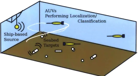
1-1 Multi-vehicle operation mission, where a fixed source insonifies a target field while multiple AUVs sample the bistatic scattering fields around various targets. 22 2-1 Insonification of a target results in acoustic scattering, as the target

re-radiates the signal in multiple echos that interfere to form the radiation pat-tern exploited by the characterization techniques discussed in this thesis. . . . 28

2-2 Simulated scattered field data at several depths. . . . 30

2-3 Simulated scattering amplitude dependence on angle

6

for spherical and cylin-drical targets.

6

is calculated by setting the target at (0, 0) and the source at

(-60, 0) such that the source is at 180". . . . 31

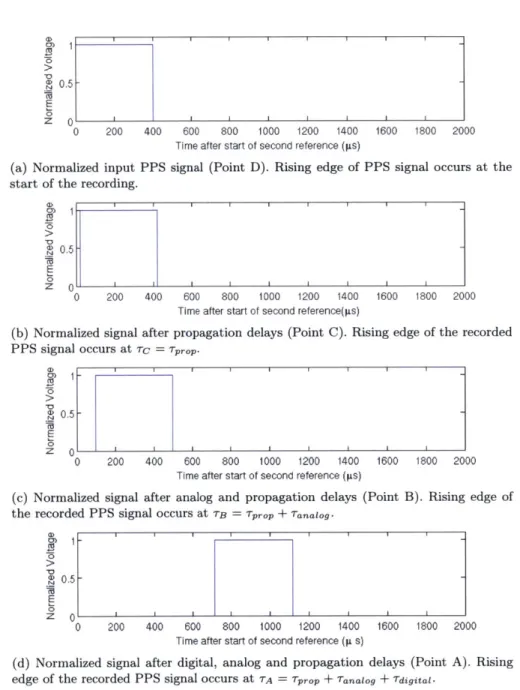
2-4 Simulated radiation patterns for spherical and cylindrical targets. The pat-tern was calculated by taking the mean intensity in each 5 degree azimuthal bin across range and depth (20-40m range, 1-4m depth), converting to dB and subtracting the minimum intensity. These polar plots are shown as looking from above on the target, with the target at (0,0) and the source at r=60, 6 = 1800 . . . . 33 2-5 Mean radiation patterns for different cylinder rotations. The location of

min-ima and maxmin-ima within the patterns shift with the angle -y. . . . 34

2-6 Intensity-averaged radiation patterns for acoustic scattering from anisotropic rough bottom patches with varying values of y = 450, depths 10-50m, ranges

20-50m . . . . 35 3-1 Block Diagram of the data aquisition and timing system. . . . 39

3-2 Experimental setup with test points. . . . 42

(14)

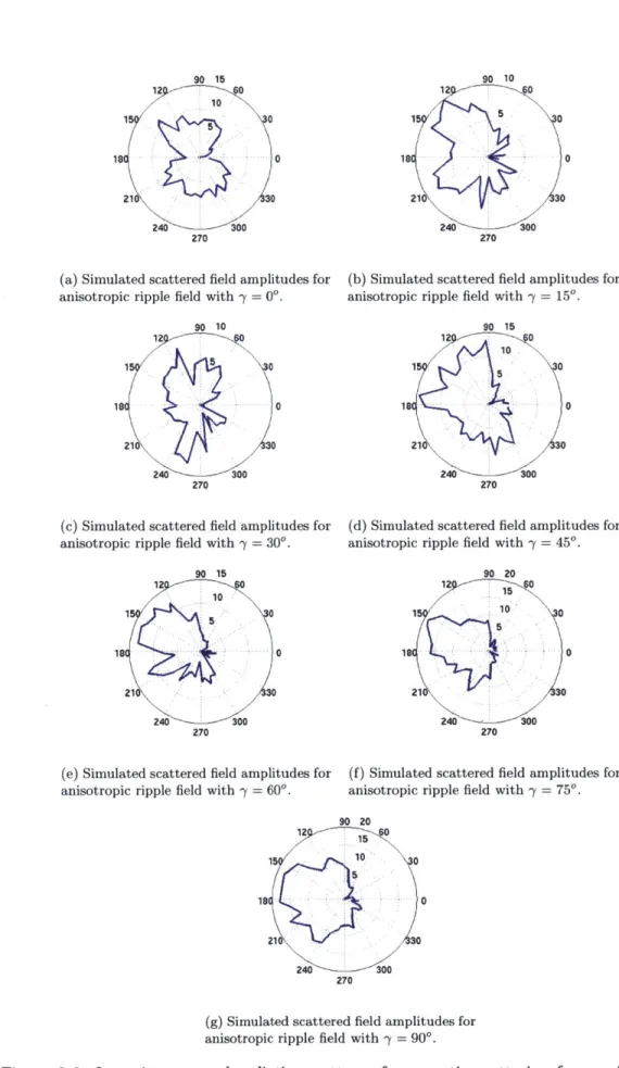
3-4 Example correlation plot showing the cross-correlation between the input PPS signal and signal at point C versus lag in seconds. . . . 47

3-5 Example recording of signal measured at point A versus the direct PPS Signal. 47 3-6 Measuring phase difference between channels. . . . 49

3-7 Plot of measured TA versus Ping Number. . . . 50

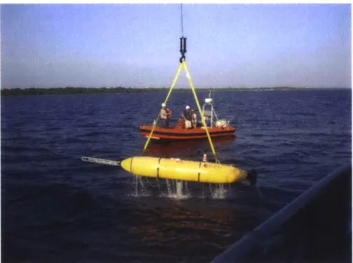
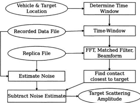
4-1 The AUV Unicorn being lifted from the water by the crane of the PCS-12 during the BayEx'14 experiment. . . . 54 4-2 Processing in pActiveTargetProcess used to extract target amplitudes from

the array time-series. The recorded data file, vehicle/target location informa-tion, and replica are used to estimate the target scattering amplitude. .-. .. 56

4-3 Full field sampling behavior used with the vehicle Unicorn for collecting target bistatic data sets. The vehicle circles the target, changing radius in the direct forward-scatter direction. . . . 57

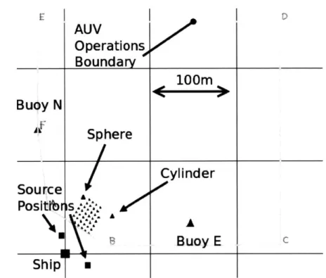
4-4 Experimental configuration, with source positions, target positions, and AUV operational box . . . .

59

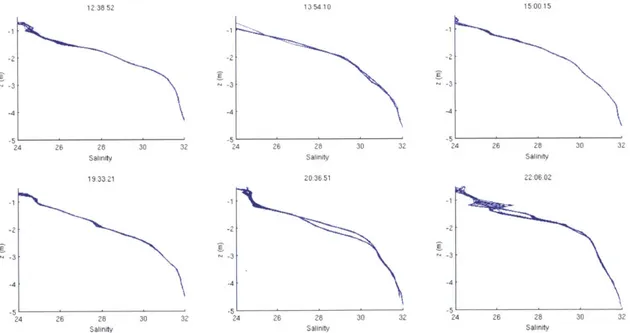
4-5 Locations of collected acoustic data files in x and y relative to the position of

the R V Sharpe. . . . 60 4-6 Salinity data collected with Unicorn on May 21 during the BayEx'14

experi-m en t. . . . . 6 1

4-7 Temperature data collected with Unicorn on May 21 during the BayEx'14 experim ent. . . . 62 4-8 Sound speed data collected with Unicorn on May 21 during the BayEx'14

experim ent. . . . 62 4-9 Sphere scattering amplitudes for depths im to 4m versus position in

target-centric coordinate system . . . 64 4-10 Cylinder scattering amplitudes for depths lm to 4m versus position in

target-centric coordinate system . . . . 64 4-11 Scattering amplitude grid around spherical and cylindrical targets, including

target positioning and cylinder rotation. Amplitudes were averaged between

2.5 and 3.5m in depth. Note the distinctive specular glint in the cylinder data

(15)

4-12 Polar plot showing angle dependence of mean target scattering amplitude for spherical and cylindrical targets. Difference between intensity-averaged amplitude and minimum amplitude is plotted on the r-axis and angle in the source-target coordinate system on the 0 axis. . . . 67 4-13 Ambient noise in dB re 1 pPa versus beamforming direction in degrees, where

beamforming is always conducted broadside to the AUV array. For example, the measurement at 0 degrees represents the noise to the east, 90 degrees to the north, and so on. The resulting noise "rose" shows nearly omnidirectional ambient noise in the 7-9kHz range. . . . 67 4-14 Configuration for Massachusetts Bay experiment, including source and

tar-get positions. The R/V Resolution, with the Lubell source deployed at 3m depth, was first anchored about 100m north of the target, then moved to approximately 100m west of the target . . . . 69

4-15 Open-ended steel pipe used as a target during the Massachusetts Bay exper-iment, sitting on the deck of the R/V Resolution. The pipe is 1.5 feet in diam eter and 5 feet long. . . . 69

4-16 Sampling for null, first and second target aspect bistatic scattering acoustic d ata sets. . . . 71 4-17 Unnormalized scattering amplitude maps for 5m depth for the two target

aspects during the Massachusetts Bay experiment. For both plots, target is located at (0,0) and source is located at approximately (-100,0). . . . 72 4-18 Radiation pattern for two target aspects sampled during the Massachusetts

Bay experiment. Arrows denote the source arrival and expected glint direction based on reflection. . . . 73 4-19 Unnormalized scattering amplitude maps for 5m depth for the first target

aspects during the Massachusetts Bay experiment and a region without a target present. For both plots, "target" is located at (0,0). The source is located at approximately (-100,0) for the first target orientation and at

(-130,0) for the null target. . . . 74

4-20 Comparison of real versus simulated scattered fields between 2.5 and 3.5m depth for spherical and cylindrical targets. . . . 76

(16)

4-21 Radiation pattern for the first aspect of the real steel pipe, estimated to have rotation 1100, versus a simulated fluid-filled cylinder with a rotation of 110'. The match is visually not very close, though there are some similarities visible in the positioning of minima and maxima. The SVM regression model was, despite the differences, able to determine that the real steel pipe was closest in orientation to the modelled 110' fluid-filled cylinder. . . . 78 4-22 Radiation pattern for the second aspect of the real steel pipe, estimated to

have rotation 36 degrees, versus a simulated fluid-filled cylinder with a rota-tion of 35 degrees. . . . 79

5-1 Training and analysis process for machine learning methodology. Acoustic scattering amplitude data is converted to a feature space and used to construct example vectors. Independent example vectors form training, validation, and test data sets. Classification model training is conducted on the training set, and the validation set is used in the selection of model parameters. The test set is then used to determine the model's generalization performance

and construct a confidence model, used to estimate the probability of correct classification given the number of samples and the classification margin. . . . 85

5-2 Angularly dependent feature space, configured using parameter

AO.

. . . 87 5-3 Classification processing chain run onboard an AUV. . . . 91 5-4 Real-time classification processing chains for runtime and simulation. . . . 92

5-5 Selection of AO based on the minimum margin ratio, /min, at increasing values of N.

AO

= 90 was selected because it converged most quickly to 3

min = 00

as the accuracy reached 100% . . . 93

5-6 N versus accuracy for model trained on real and simulated data with feature

space where AO = 90. As N increases, the accuracy increases until it reaches

100%. This behavior is expected, as additional data improves the averaging

in each feature. After N = 190 the accuracy goes to 100%. When N = 190,

the vehicle has generally completed two circles of the target. . . . 94

5-7 Classification confidence versus margin and N for sphere versus cylinder

(17)

6-1 Schematic on the use of an AUV for estimation of a target's aspect using sampled bistatic acoustic scattered field data. Like in the Massachusetts Bay experiment, a ship-based source insonifies a target using a 7-9kHz signal as an

AUV sampled the resulting scattered field and uses the collected amplitude

data to estimate the orientation angle of the target relative to the source. . .100 6-2 Schematic on the use of an AUV for estimation of anisotropy using sampled

bistatic acoustic scattered field data. A fixed source insonifies a patch on the bottom using a 1-5kHz signal, an AUV sampled the resulting scattered field and uses the collected amplitude data to estimate the anisotropy angle of ripple field. . . . 101

6-3 Training and Analysis Process. Real or simulated 3D scattered field data is used to generate sets of example vectors for training, validation and testing. The model trained with the training set is used along with the validation set to select SVM model parameters. The test set is used to asses model viability. 106 6-4 Real-time regression process. Once the regression mode is initialized on a

vehicle, the SVM model produced in the training/analysis phase is used to estimate the angle and the confidence of that estimate. . . . 107

6-5 Real-time regression processing chain in MOOS-IvP simulation environment. Multipath arrivals are simulated on array by uSimActiveSonar. That data is processed in real time using pActiveTargetProcess to extract target ampli-tudes. When the selected target's contact is present, uSimScatt outputs the appropriate scattered field amplitude for pProcessScatt. pSVMRegress esti-mates the angle from the resulting example vector as new data is acquired. It also estimates the probability that that estimate has an error less than d degrees, where d is configurable. . . . 109

6-6 Probability density function over estimated angle for varying values of N for the two target orientations. The first orientation converges to a value of

~ = 1100, the second to a value of ~Y = 350 . . . . 111

6-7 Example Anisotropic Goff-Jordan rough bottom ripple fields and resulting scattered fields. . . . 113

(18)

6-9 P( dmaxI < m), calculated by finding the percentage of paths that resulted in

less than m degrees error from regression of the test set X,. The curve shows

the characteristics of a Gaussian CDF. . . . 117

6-10 True anisotropy angle -y versus estimated anisotropy angle ' for paths in test set Xx that resulted in maximum anisotropy error of less than 30. Each blue line represents the anisotropy estimation values for a single geometric sampling applied across the tested anisotropy angles. The red line represents a perfect regression result, where -( = . . . . 118

6-11 PDFs of anisotropy error, fD(d), versus anisotropy error in degrees, d, for several values of N from analysis of error data. Note that the error is clearly Gaussian in distribution and as the time spent sampling the scattered field increases, the standard deviation decreases while the mean remains approx-imately the same. Gaussian models were fit to this data to estimate mean and standard deviation for different numbers of samples and used to estimate confidence... ... 120

6-12 The log-log linear relationship between the number of samples N and the standard deviation of the PDF of the error,

o-.

The circles show the values derived from the data, and the line shows the least squares best fit of log(a) = -0.44 log(N ) + 4.64. . . . 121

6-13 Simulated AUV circling a simulated insonifies bottom patch, with SVM Re-gression for estimation of anisotropy angle . . . 122

B-i Uniform feature space geometry. Values of rstep, zstep and 6 step are selected using a reducing grid search. . . . 137

B-2 Comparison of performance of three tested feature spaces. . . . 141

C-1 Autogeneration process to produce SVM files for simulation data. . . . 144

(19)

List of Tables

3.1 Timing characterization variables . . . 43

3.2 Delays and Calibration Constants . . . 49

4.1 Target Geom etry. . . . .

58

6.1 Variables used to describe regression for angle estimation. . . . 124

6.2 Parameters for target scattering simulations for cylinder regression. . . . 124

(20)

(21)

Chapter 1 Introduction

1.1 Motivation

A growing application for Autonomous Underwater Vehicle (AUV) technology is the

local-ization, classification and mitigation of underwater hazards in shallow harbor environments. The classification problem has attracted particular attention in recent years with the de-velopment of visual and acoustic AUV-based sensors for remote data collection. Because visual inspection of targets can be difficult or impossible in murky harbors and requires precise target localization, acoustic sensors such as sidescan sonar and synthetic aperture sonar (SAS) are used more extensively for AUV-based Mine Countermeasures.

At the current level of technology, these techniques can provide rich images of targets and the environment but produce data that are difficult to use for real-time target classifica-tion. Sidescan sonar systems are generally too high frequency for buried target localization and classification. SAS images are usually computed in post-processing so that naviga-tion correcnaviga-tions may be applied [1]. The current operanaviga-tional paradigm for the use of both technologies requires a human in the loop for expert image interpretation. In addition to these challenges to fully autonomous real-time classification of data from these systems, the sensors themselves are too expensive to be practical in multi-vehicle operations.

To achieve plausible, real-time AUV-based target classification that is expandable to distributed vehicle networks, two key advancements are required: an inexpensive sensing payload and a classification method that can be run in real-time on an AUV computer using onboard processing of sensor and navigation data. The advantages of such a sensing system would be the ability to deploy multiple AUVs to carry out the target localization

(22)

Figure 1-1: Multi-vehicle operation mission, where a fixed source insonifies a target field while multiple AUVs sample the bistatic scattering fields around various targets.

and classification missions with immediate classification and confidence estimates to inform prosecution decisions without having to recover and redeploy vehicles.

The goal for this thesis was to develop a payload and processing chain for target classifi-cation using only bistatic acoustic data collected on an AUV's linear hydrophone nose array cut for low-frequency acoustic sensing (1-15kHz). The bistatic configuration and hydrophone array were selected to limit sensing system cost: in the multi-vehicle scenario, a fixed acous-tic source insonifies a target field while multiple vehicles with inexpensive payloads collect bistatic scattering data around targets, as shown in Figure 1-1.

This thesis presents the AUV payload required to perform bistatic acoustic data collec-tion, real-world bistatic acoustic data sets collected around spherical and aspect-dependent seabed targets with that payload, and a machine-learning methodology that utilizes bistatic angle dependence of amplitude features from the scattered field to classify target shape and estimate the orientation of aspect-dependent targets. This approach was highly successful for the classification of spheres versus cylinders and for the estimation of target orientation. The results from real and simulated data for simple target geometries suggest that using fea-tures of the bistatic acoustic scattering radiation pattern for target classification in real time on AUVs is a plausible solution to the real-time target classification problem and warrants further study.

AUVs

Performing Localization/

Classification

Ship-based

Sourc

(23)

1.2 Historical Background

1.2.1 Bistatic Scattering from Seabed Targets

The vast majority of target scattering literature is focused on backscattering data from monostatic sensing. However, there is a small body of theoretical and experimental work looking at the bistatic scattering problem.

Bistatic scattering theory and models have been developed for simple target geometries (sphere, spheroid, cylinder) in simple environments. The theoretical and numerical work on bistatic scattering from spheres includes that by Gaunaurd and Uberall

12],

which discusses the free field bistatic form function of spherical targets and gives an example numerical calculation. Hackman and Sammelmann describe the theoretical scattering from a spheroidal target in an ocean waveguide, and include numerical results for the bistatic case [3]. While the backscatter from finite cylinders for various aspects has been described analytically [4] [5], the additional dimensionality of the bistatic problem means that the approach to finding the bistatic scattered field is numerical. The analytical bistatic sphere scattering formulation and Rumerman's scattering model for cylinders [6] are used in the OASES-SCATT acoustic simulation package developed by Schmidt and Lee [7]

18].

This acoustic package was used to explore effects of environment, bottom composition and target geometry on bistatic acoustic fields in Lee's thesis, "Multi-static Scattering of Targets and Rough Interfaces in Ocean Waveguides"

[9].

Virtual scattering experiments using the

OASES-SCATT scattering simulator influenced this work by showing clear distinctions in bistatic

target scattering field characteristics.

Most of the limited experimental work on bistatic target scattering has been conducted in the small scale, in water tanks and test ponds. For example, Baik, Dudley, and Marston conducted an experiment where they looked at the bistatic response of different cylinders in a test tank for the purposes of holographic imaging

[10].

Kargl et. al. looked at the bistatic scattering response of aspect-dependent targets in a test pond as a part of the PondEx10 experiment [11].

These experiments used moveable arrays that are not easily adapted to a harbor environ-ment, and there have been very few attempts to collect bistatic acoustic data in situ with AUVs. The GOATS'98 experiment is a rare example of a successful AUV-based bistatic scattering experiment: it included an AUV with a nose array, and produced data on the

(24)

bistatic scattered fields off of fully buried, partially buried and proud spheres. Lepage and Schmidt

[12]

and Edwards et. al.

[131

describe the AUV experiment and using the array data for Synthetic Aperture Sonar imaging. Synchronization was achieved using a vehicle-based acoustic signal to trigger the source. The data was collected using lawnmower patterns through the target field, which had the disadvantage of giving non-uniform data quality and few data with the array at broadside to each target. The significant advances in many areas since 1998 made a new experiment to collect bistatic data with an AUV valuable. These areas of tremendous advancement include the computational power for real-time tar-get tracking and classification, adaptive autonomy to allow more efficient data collection, the existence of small, low-power, high-accuracy clocks for synchronization timing, and vehicle navigation with less than 0.5% drift per distance travelled.

1.2.2 Target Classification

The more recent literature on using AUVs for Mine Countermeasures classification tasks focuses on the use of monostatic and imaging techniques, often in high frequency. Examples of these techniques include Synthetic Aperture Sonar (SAS) and sidescan sonar. These methods have been shown to be effective for many target types and circumstances, but the expense of developing and deploying these systems as well as the difficulty of using the resulting data for real-time classification justifies investigation into alternative methods. The AUV-based SAS work does not utilize the true bistatic field, but uses an array and source together on an AUV to get a synthetic aperture, simplifying navigational constraints. There are very few examples of using a SAS imaging approach with bistatic data: it was attempted by Edwards et. al. as a part of the GOATS'98 experiment

1131

and discussed in a paper by Dudley and Marston, for experimental data collected using a rail source and receiver [141.

Monostatic target classification using probabilistic methods is discussed in

[15],

which attempts to classify targets using multiaspect backscatter, wave-based signal processing and Hidden Markov Models (HMMs). In this method, a model is trained and then used to classify new targets. This work demonstrates an empirical model-based approach to target classification with a geometric feature space, though methods described use only backscatter data, utilize a different aspect of the acoustic signal, and do not use a machine learning approach to the classification.

(25)

Several machine learning based target classification methods using backscatter informa-tion and a frequency or time-frequency analysis of the target return have been published. Kaminsky and Barbu looked at classification of buried cylindrical targets (such as cables) using simulated data and a discriminant analysis method applied to a time-frequency im-age

[161.

Malarkodi et. al. investigated using Neural Networks for classification of target type using a features space that was a statistical representation of the target return power spectrum for a 40-80kHz Linear Frequency Modulation (LFM) chirp [17]. These techniques differ from those described in this thesis in that they use features that include temporal or phase information and only look at monostatic data.

1.3 Contributions

There are two important contributions of this thesis. The first is the bistatic data set collected during the BayEx'14 and Massachusetts Bay experiments and the development of the AUV payload for collecting that data. The second is the use of bistatic angle dependence of scattering amplitudes with a machine learning methodology for target characterization, which was demonstrated on simulated and real bistatic scattering data for the classification spheres versus cylinders and for the estimation of rotation angle for aspect-dependent targets and sand ripple fields.

Initial simulation studies provided the inspiration for using the relationship between scattering amplitude and bistatic angle as a basis for target classification. Chapter 2 explains some of the basic principles of target scattering, with supporting examples from simulation. As discussed in the Historical Background section, very few bistatic scattering experi-ments have been conducted in real harbor environexperi-ments with AUVs. The challenges to a successful AUV-based bistatic scattering experiment included timing, navigation, and col-lecting uniform-quality data. Chapter 3 describes the acoustic payload designed and built for precision timing of data acquisition on the AUV Unicorn for bistatic scattering experi-ments and the characterization experiexperi-ments undertaken to ensure that timing requireexperi-ments were met. Chapter 4 then explains the combination of hardware, signal processing, and vehicle behaviors used to collect dense, high-quality bistatic scattering data sets around spherical and simple aspect-dependent targets during the BayEx'14 and Massachusetts Bay experiments using the AUV Unicorn. The resulting data sets are presented and compared

(26)

to predicted scattering results from simulation. Chapter 5 explains the machine learning classification methodology developed to use the geometric pattern of bistatic scattering am-plitudes to distinguish spherical from cylindrical targets. The results from applying this methodology on real and simulated data are then described, including features space and parameter selection algorithms.

Chapter 6 describes the extension of the machine learning classification methodology to regression problems for the estimation of cylinder rotation angles and seabed ripple field anisotropy.

(27)

Chapter 2 Object Scattering In The Ocean

2.1 Overview

When a target on the ocean bottom is acoustically insonified, the target re-radiates the signal (Figure 2-1). This reradiation consists of multiple time delayed echos that interfere in the frequency domain.

For the problem of classifying underwater targets in real time using data collected on an

AUV, it was critical to identify features that were robust to several meters of error in vehicle

location, source location, and target location. The combined navigational uncertainty, plus the computations limitations for data processing on an AUV, made using sensitive time and phase information for target classification impractical. While these features are frequently used for SAS imaging, they would be difficult to use in real time on a bistatic AUV system because of the navigation errors inherent in an AUV system.

The interference of the time-delayed echos from target scattering result in frequency-dependent minima and maxima in the bistatic radiation pattern from the target. These scattering radiation patterns are distinct for different target types and are mostly dependent on the bistatic angle of an amplitude measurement, showing range and depth independence over meters or tens of meters. Bistatic angle is the angle between the source and the receiver relative to the target. The concept for the classification techniques discussed in this thesis is that these interference patterns in a given frequency band are stable and can be used to characterize seabed targets.

The technology required for getting data on the bistatic radiation pattern is an AUV with a linear hydrophone nose array, a data acquisition system, and signal processing software to

(28)

Acoustic Source

0 Seabed

Target

Figure 2-1: Insonification of a target results in acoustic scattering, as the target re-radiates the signal in multiple echos that interfere to form the radiation pattern exploited by the characterization techniques discussed in this thesis.

calculate target scattering amplitude as acoustic data is collected around a target. Imaging techniques are not required, as the dependence of scattering amplitude on bistatic angle can be analysed directly.

2.2 Modelling Target Scattering with Wavenumber

Integra-tion

The wavenumber integration computational approach involves decomposing the acoustic field in frequency and wavenumber, which makes it a good technique for propagation of target scattering fields, as the dependence of the scattering radiation pattern is in the frequency domain. While the models do not include multiple scattering or elastic scattering effects, real scattering data showed the simulations to be generally effective at predicting the radiation pattern for different targets and environments.

The OASES-SCATT scattering simulation package was used extensively in this thesis for modelling target and bottom roughness scattering fields

[71

181.

This simulation package uses the single scattering approximation

118],

assumes an incident plane wave, and approximates the target as a virtual point source with a specific radiation pattern[9]. The single scattering approximation could be insufficient for accurately modelling temporal features of target scattering, but is adequate for modelling minima and maxima of the interference pattern,

(29)

of greatest interest in this thesis [7]. The plane wave approximation is appropriate for the scenarios considered here as the source is in the far field from the target. Effects due to layers in the medium are taken into account in the wavenumber integration approach, so waveguide effects are included in the resulting models.

The simulation package uses 2-D wavenumber integration to propagate a plane wave from the source to the target location. The equivalent virtual source radiation pattern is then calculated for the target. For spheres, a volume scatterer approximation is used to directly calculate the scattered pressure field from the incident pressure and boundary conditions. Rumerman's scattering model [6] is used to calculate the effective source function for finite cylinder shells. 3-D wavenumber integration is then used to compute the full 3-D scattering field from the spectral radiation pattern of the target at a set of ranges and depths for the specified environment. The final output includes the azimuthal Fourier orders for a series of ranges and depths from the target. In addition to target simulation, the scattering package can model rough bottom scattering. This was used for modelling of anisotropic sand ripple field bottom scattering to provide a second example of regression for parameter estimation Section 6.3.

To interface the scattering simulation package with classification and regression soft-ware, the custom AutoGen code was written. This code has a database back end that allows reconstruction of all simulation experiments based on input parameters, and was used for automatic generation of scattering fields based on target, source and environment configuration. Appendix C describes this code in detail.

2.2.1 Target Scattering

The target scattering simulator was used to generate scattering models for the simple target geometries used in this thesis. The assumptions about the target radiation patterns that underlie this thesis were based on simulation data. The most important of these are the persistence of radiation pattern features between ranges and depths for a given frequency. Figure 2-2 shows the simulated scattering amplitudes for spherical and cylindrical targets in a 6.5m deep waveguide for multiple depths, generated using the BayEx'14 configuration shown in Appendix A. The source is 3m deep, 8kHz, and 60m from the target. The simulated water depth is 8m, with a mud bottom over sand.

(30)

40 20 0 160 150 140 130 120 -40 -20 0 20 40

(a) Simulated scattered field amplitudes for sphere, depth=1m. 40U * 160 20

U

150 0 140 E130f

I

120 -40 -20 0 20 40 (c) Simulated scattered field amplitudes sphere, depth=2m. 40

1160

for 140

I

120 -40 -40 -20 0 20 40

(e) Simulated scattered field amplitudes for sphere, depth=3m. . 1160 C 140 120 -40 -20 0 20 40

(g) Simulated scattered field amplitudes for

sphere, depth=4m. 0 160 140

I

120 -40 -20 0 20 40

(b) Simulated scattered field amplitudes for

cylinder, depth=1m.

2* 1160

140

I

120

-40 -20 0 20 40

(d) Simulated scattered field amplitudes for

cylinder, depth=2m. 40

20 A

ISO

0 140 -2012

1120

-4017 -40 -20 0 20 40

(f) Simulated scattered field amplitudes for

cylinder, depth=3m. 160 0 140 -0120 -40 -20 0 20 40

(h) Simulated scattered field amplitudes for cylinder, depth=4m.

(31)

CUO :160 S160 14014 .) 0) S120 120 0 10i 100 0 2 4 6 0 2 4 6 0 (radians) 0 (radians)

(a) Dependence of scattering amplitude be- (b) Dependence of scattering amplitude

be-tween ranges of 20 and 40m for spherical tween ranges of 20 and 40m for cylindrical

target. target.

Figure 2-3: Simulated scattering amplitude dependence on angle 0 for spherical and cylin-drical targets. 6 is calculated by setting the target at (0, 0) and the source at (-60, 0) such that the source is at 1800.

amplitude minima and maxima in the scattered field. These features are only slowly changing with depth and generally consistent in range from the target. The lobes of the radiation pattern are also meters wide in the far field. Figure 2-3 shows the dependence of scattering amplitude on bistatic angle, 6, across all depths and 20-40m range for the sphere and cylinder case. The general location of minima and maxima within the pattern remains consistent with different depths and ranges. These properties would make sensing of the overall radiation pattern robust to several meters of AUV navigation error. Utilizing scattering amplitude information has the additional advantage of being more robust to noise and interference than temporal or phase information. Figure 2-4 shows the intensity-averaged radiation pattern for spherical and cylindrical targets versus bistatic angle. Represented in this fashion, the difference between the two target types is very clear, providing a good basis for AUV-based target classification.

The aspect-dependence of cylindrical targets also causes distinct features in the bistatic angle dependence of the radiation pattern. Figure 2-5 shows several cylinder rotations to aspect angle -y relative to the source and the resulting simulated radiation patterns versus azimuthal angle relative to the source. The location of minima and maxima shift with aspect angle, suggesting that the orientation of a cylinder could be estimated using a regression model.

(32)

2.2.2 Ripple Field Scattering

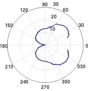
Similarly, the scattered fields from anisotropic bottom ripple fields have their most major features in azimuth, rather than range and depth. Figure 2-6 shows the impact on the radiation pattern of the anisotropy angle. Like with cylinder orientation, the radiation pattern shifts consistently in a way that suggests the anisotropy angle could be estimated using a regression model. These scattering simulations assumes a 100m waveguide with a source at 30m depth, 100m from the insonified bottom patch. Within a 20-50m set of ranges and 20m of depth, the location and strength of minima and maxima are consistent and persistent. The mean or median scattering amplitude dependence on anisotropy angle is distinctive.

2.3 Conclusions

Simulation experiments using a wavenumber integration-based scattering simulation pack-age suggested that the dependence of target scattering amplitude on bistatic angle provides robust features that could be used for target characterization. The use of these features, rather than time or phase-based information, loosens navigation accuracy requirements to what is plausible on an AUV. Additionally, target scattering amplitudes can be calculated directly from acoustic data collected on a line array carried by an AUV. Utilizing the de-pendence of target scattering amplitude on the bistatic angle of sampling does not require sophisticated imaging techniques for classification, and could provide a basis for onboard target characterization.

(33)

90 30

12

30

270

(a) Intensity-averaged radiation pattern, averaged over range and depth, for spherical target.

90 30

15

30

0

210

30

240

300

270

(b) Intensity-averaged radiation pattern, averaged over range and depth, for cylindrical target.

Figure 2-4: Simulated radiation patterns for spherical and

cylindrical

targets. The pattern was calculated by taking the mean intensity in each 5 degree azimuthal bin across range and depth (20-4Oim range, 1-4m depth), converting to dB and subtracting the minimum intensity. These polar plots are shown as

looking

from above on the target, with the target at (0,0) and the source at r=z6O, 0 1800.

(34)

90 40 12 0 30 15 20 0 18 0 210 30 240 300 270 (a) -y = 00. 90 40 12 0 30 15 20 0 180 210 30 240 300 270 (c) = 300. 90 30 12 60 20 15 0 18 210 30 240 300 270 (e) y = 600. 90 30 12 60 20 15 0 210 30 240 300 270 (g) y = 1200. 90 40 12 0 15 20 15 0 210 30 240 300n 270 (b) -y = 15" 90 30 1 0 20 15 0 10 210 30 240 300 270 (d) = 45* 90 30 12 0 20 18 0 18 0 21 30 240 300 270 (f) = 90*. 90 30 1 60 20 1 0 18 1i1- 0 21 30 240 300 270 (h) y 1500.

Figure 2-5: Mean radiation patterns for different cylinder rotations. The location of minima and maxima within the patterns shift with the angle y.

(35)

90 15 12 0 10 15 - 5 0 is 0 21 30 240 300 270

(a) Simulated scattered field amplitudes for anisotropic ripple field with -y = 00.

90 10 12

60

15 5 0 18 0 210 30 240 300 270

(c) Simulated scattered field amplitudes for anisotropic ripple field with -y = 30'.

90 15 12 0 10 15 0 180 21 30 240 300 270

(e) Simulated scattered field amplitudes for anisotropic ripple field with -y = 60'.

90 10 12 60 15 0 18 0 21 30 240 300 270

(b) Simulated scattered field amplitudes for

anisotropic ripple field with -y = 15'.

90 15 12 60 10 15 0 18 0 210 30 240 300 270

(d) Simulated scattered field amplitudes for

anisotropic ripple field with -y = 45*.

90 20 12 0 15 15 10 0 18 1 0 21 30 240 300 270

(f) Simulated scattered field amplitudes for

anisotropic ripple field with - = 75*.

90 20 12 60 15 10 0 0 210 30 240 300 270

(g) Simulated scattered field amplitudes for

anisotropic ripple field with -y = 90*.

Figure 2-6: Intensity-averaged radiation patterns for acoustic scattering from anisotropic rough bottom patches with varying values of -y = 450, depths 10-50m, ranges 20-50m.

(36)

(37)

Chapter 3 Acoustic Payload

To show that reliable bistatic scattering data collection by an AUV was feasible, an acoustic payload had to be designed and built that solved the problem of time synchronization between the acoustic source and vehicle. There were a number of obstacles to achieving the required data logging accuracy. First, while many surface-based systems use global position systems (GPS) to synchronize a local clock to the satellite pulse-per-second (PPS) signal, this microsecond-precise clock was not available underwater. Second, the computer clock, even synchronized via Network Time Protocol (NTP) to a precise PPS signal, has accuracy only in milliseconds, and therefore could not be used to trigger data collection when desired accuracy was in microseconds. Third, delays introduced by analog filters and analog-to-digital conversion were in the tens to hundreds of microseconds, and had to be taken into account in system calibration to achieve sufficient system accuracy. This chapter presents the implementation of an accurate and precise data acquisition system for bistatic acoustic data collection on an AUV using off-the-shelf hardware and a set of test routines for calibration. First, the application is explained and the commercial off-the-shelf hardware is described. The payload architecture is then laid out, including hardware and software implementation needed for a functioning precision-timed data acquisition system. Next, the test procedures used in the characterization and calibration of the system to eliminate system delays are explained. Finally, the results and conclusions, including total system accuracy, are reported.

(38)

3.1 Background

In general, one of the greatest challenges to remote sensing in the ocean is the problem of maintaining adequate time synchronization between the shore and any submerged system

119).

Similarly, one of obstacles to the practical collection and use of bistatic scattering data was vehicle-source time synchronization. The absolute start time of each acoustic data file had to be known so that the target scattering signature could be identified within the time series. This required synchronizing the firing schedule of the acoustic source with the data acquisition system on-board the vehicle. There were two types of accuracy required of the data acquisition system for this acoustic experiment: accuracy in arrival time of a contact and accuracy in phase between channels in the hydrophone array. The desired resolution in range for this system was 0. im, which corresponds to a 70 microsecond difference between the true and estimated time that the file begins recording. Less accurate time synchronization would results in poor resolution of target range, which could cause misestimation of target scattering strength by onboard signal processing. Similarly, the 16 channels need to start recording at the same time so that the phase shifting between the channels is introduced

by the signal directionality rather than recording delays. The maximum permissible delay

between channels in the system was one percent of a wavelength amount, approximately 1 microsecond at 9kHz, to ensure that phase shifts introduced by recording delays did not affect beamforming operations used to calculate the arrival direction of the signal.

3.2 Payload Architecture Overview

The acoustic payload used in the AUV Unicorn for this experiment consisted of the 16 element linear nose array used to collect acoustic data, a preamplifier for filtering and am-plification on the raw signal, two 24DS112-PLL data acquisition boards (DABs) [201 for analog-to-digital conversion and an Advantech 3363 computer [211 with Intel Atom dual core processor for data logging, signal processing, and vehicle autonomy. A Quantum Chip Scale Atomic Clock (CSAC) SA.45s provided an accurate on-board time reference, and was synchronized using the time reference from a Garmin 15xLW GPS while on the surface. Figure 3-1 shows how these parts of the data acquisition and timing system interact. The analog signals from the 16 elements of the hydrophone array were filtered and amplified by the preamplifier, then synchronously recorded as 24-bit digital by the DABs. This recording

(39)

was triggered by the rising edge of the CSAC PPS signal. The digital data is sent in the form of a first-in-first-out (FIFO) buffer over PCI bus to the Advantech 3363 computer, which ran a daemon that controls the DABs and logs the data to a timestamped file.

Payload

16 Channels

From _{y-> Preamp -*Data Aquisition_} Boards

CSAC PPS FIFO Stream

Nose Array Section AUV Unicorn

Figure 3-1: Block Diagram of the data aquisition and timing system.

3.2.1 Real-Time Clock Synchronization

The

Quantum

CSAC SA.45s is a high-precision,

low-cost,

low-power clock well suited for underwater sensing platforms, including autonomous underwater vehicles. A CSAC, prop-erly aged, can be considered a reliable time source with precision

limited

by its drift rate and an accuracy limited by the accuracy of the global time source it uses as a synchroniza-tion reference. The aging rate of the CSAC is 3.OE-1/month [22], which far exceeds the requirements of this application, where vehicles are deployed for

less

than a day at a time.

A CSAC and CSAC development board were integrated with the computer and acoustic data acquisition systems in the AUV payload to provide a precision pulse-per-second time reference while the AUV was submerged. The addition of a Garmin 1xLW GPS to the payload, connected to an external GPS antenna, provided a time of day and PPS reference for CSAC synchronization on the surface. Synchronization set the rising edge of the CSAC Board's PPS output to match the rising edge of the GPS PPS so that the start-of-second time reference was the same.

(40)

was managed using a custom daemon, which ensured that the vehicle and source time references were the same. This daemon had two critical functions: to perform GPS-CSAC synchronization on startup (if satellites are available), and to provide a GPRMC NMEA message to the vehicle computer. The NMEA sentence was used by the generic NMEA

GPS Receiver (reference clock 20

123])

for setting the LinuxPPS

[24]

reimplementation of the NTP server on the computer. Since the timing of the recording relative to the start of the second was known, if the computer clock was on the correct second when the data was recorded the file's timestamp was correct.

A backup power system for the CSAC was built so that the system could remain

contin-uously on. This was important because the CSAC's performance improves as it ages [22]. Four hot-swap circuits provided automatic switching between three power sources: an on-board battery pack containing 3 AA batteries, the regular vehicle power source, and an externally accessible CSAC-only 5V power line. In ordinary operations, the vehicle could be shut off and the external CSAC power then connected without opening the payload or removing it from the vehicle. The battery pack, which lasts for more than 24 hours as the only power source, kept the CSAC running during this changeover.

3.2.2 Data Acquisition

To achieve the level of accuracy in time synchronization required by this experiment, data recording and logging had to properly implemented, using the CSAC PPS as a hardware trigger. This was necessary because NTP provides, in the best-case, 1 millisecond accuracy due to the drift in the real-time clock and the general delays in a non real-time operating system.

8 channels from the preamplifier passed into each of the system's two DABs. These

boards converted the analog voltages into 24 bit digital data at a sampling rate of 37500Hz, and wrote the resulting binary data to the PCI bus FIFO buffer to be read on the payload computer.

The DABs were configured to run synchronously across all channels and to use the GPS lock feature. This meant that all channels were recorded at the same time, such that the first 8 samples in the FIFO buffer correspond to the voltage level received on 8 elements in the same time bin. GPS lock mode guaranteed that exactly the configured samples per second were recorded each second, re-setting the lock state if there was a drift of more than

Characterization of underwater target geometry from autonomous underwater vehicle sampling of bistatic acoustic scattered fields

Characterization of Underwater Target Geometry from

Autonomous Underwater Vehicle Sampling of Bistatic

Acoustic Scattered Fields

by

Erin Marie Fischell

Submitted to the Joint Program in Applied Ocean Science & Engineering

in partial fulfillment of the requirements for the degree of

Doctor of Philosophy

at the

MASSACHUSETTS INSTITUTE OF TECHNOLOGY

and the

WOODS HOLE OCEANOGRAPHIC INSTITUTION

June 2015

@2015 Erin M. Fischell.

All rights reserved.

ARCHNES

JUL 3

0

2015

LIBRARIES

The author hereby grants to MIT and WHOI permission to reproduce and to

distribute publicly paper and electronic copies of this thesis document in whole or in

part in any medium now known or hereafter created.

Signature redacted

Joint Program in Applied Ocean Science & Engineering

Massachusetts Institute of Technology

& Woods Hole Oceanographic Institution

March 27, 2015

Certified by...

Signature redacted'

Signat

AU f

Henrik Schmidt

Professor of Mechanical and Ocean Engineering

Massachusetfs Institute of Technology

u re reda

,acted

fhesis Supervisor

A ccep ted b y ...

David E. Hardt

Chairman, Committee for Graduate Students

Accepted by

M

ch

t

Institute of Technology

.Signature

redacted ...

Henrik Schmidt

Chairman, Joint Committee for ApplieKOcean Science & Engineering

Massachusetts Institute of Technology

Characterization of Underwater Target Geometry from Autonomous

Underwater Vehicle Sampling of Bistatic Acoustic Scattered Fields

Abstract

Biography

Acknowledgments

Contents

List of Figures

6

6

59

AO.

AO

o-.

List of Tables

58

Chapter 1

Introduction

1.1

Motivation

AUVs

Performing Localization/

Classification

Ship-based

Sourc

1.2

Historical Background

1.2.1

Bistatic Scattering from Seabed Targets