HAL Id: hal-01577180
https://hal.archives-ouvertes.fr/hal-01577180
Submitted on 25 Aug 2017
HAL is a multi-disciplinary open access
archive for the deposit and dissemination of
sci-entific research documents, whether they are
pub-lished or not. The documents may come from
teaching and research institutions in France or
abroad, or from public or private research centers.
L’archive ouverte pluridisciplinaire HAL, est
destinée au dépôt et à la diffusion de documents
scientifiques de niveau recherche, publiés ou non,
émanant des établissements d’enseignement et de
recherche français ou étrangers, des laboratoires
publics ou privés.
EvoEvo Deliverable 5.2
Guillaume Beslon, Jonas Abernot, Sergio Peignier, Christophe Rigotti
To cite this version:
Guillaume Beslon, Jonas Abernot, Sergio Peignier, Christophe Rigotti. EvoEvo Deliverable 5.2:
Im-pact obtained from EvoEvo mechanisms on evolution of a hardware personal companion. [Research
Report] INRIA Grenoble - Rhône-Alpes. 2016. �hal-01577180�
FP7-ICT FET Proactive EVLIT program EvoEvo personal companion application
Project reference: 610427 Version 1.2
EvoEvo Deliverable 5.2
Impact obtained from EvoEvo mechanisms on evolution of a
hardware personal companion
Due date: M36
Person in charge: Guillaume Beslon
Partner in charge: INRIA
Workpackage: WP5 (EvoEvo applications)
Deliverable description: Impact obtained from EvoEvo mechanisms on evolution of a hardware personal companion: A report on the development and results of the evolvable personal companion. The report should identify the strengths and weaknesses of the EvoEvo approach for this application.
Revisions:
Revision no. Revision description Date Person in charge
1.0 First version 24/10/16 J. Abernot - S.
Peignier (INRIA)
1.1 Corrections and complement 28/10/16 C. Rigotti (INRIA)
Abstract This report presents the EvoMove musical companion that generates music according to performer moves. It uses wireless sensors (accelerometers, gyroscopes and magnetometers) to acquire a continuous stream of information about the motions of the performer. This stream is analyzed on-the-fly to exhibit categories of similar moves and to iden-tify the category of new incoming moves. The main feature is that these categories are not predefined but are determined in a dynamic way by a new subspace clustering algorithm. This algorithm, called SubCMedians, stems from our previous work on the Chameleoclust+ algorithm (Deliver-able 5.1) and is targeted towards more efficient processing. SubCMedians is a median-based subspace clustering algorithm using a weight-based hill climbing strategy and a stochastic local exploration step. It is shown to exhibit satisfactory quality clusters when compared to well-established clustering paradigms, while allowing for fast on-the-fly handling of the sensor data. The music generation itself relies on a tiling over time of audio samples, where each sample is triggered according to the moves detected in the data stream coming from the sensors.
1
Introduction
This report describes a prototype system built to explore potential real-world applications of EvoEvo inspired technologies. As described in section 6.3.1 of the mid-term dissemination report (Deliverable 6.5), we aimed at building a personal companion that is a musical system able to produce music on-the-fly from the moves/dance of a performer. This system is named EvoMove, and its hardware is composed of several parts: (1) wearable motion sensors, (2) an acquisition gateway, (3) a move recognition unit and (4) a sound generator.
The first aim of this work is to assess the efficiency of the technology inspired by EvoEvo : Can it handle real noisy data ? Can it process them on-the-fly ? Is it able to keep on evolving over this motion stream ? Is its adaptation able to handle such an open-ended context ? In addition, these experiments provide also a first insight into the interaction between human users and this self-adapting technology.
The EvoMove system uses a subspace clustering algorithm (e.g., [7], [9], [10]) as a move categorization/recognition subsystem. This algorithm, named SubC-Medians, comes from the expertise acquired during the development and use of the evolutionary algorithm Chameleoclust+ (Deliverable 5.1). SubCMedians is a complete redesign, incorporating important changes in the evolution model itself, so as to be adapted to on-the fly processing of the data. In particular, it relies on more abstract mutational operations and avoids the explicit representation of the full genome structure.
The performer moves are captured via a set of wireless sensors that combine accelerometers, gyroscopes and magnetometers1, built by the HIKOB company (www.hikob.com). The sensors are worn by the performer and the data are col-lected by a gateway component that must be located within a distance of a few
1
tens of meters from the performer. The communication architecture to query this gateway relies on a client-server model, allowing thus to deploy a variable number of sensors, and even to set them on several performers at the same time. The architecture of the system is described in figure 1: (A) Data produced by the performer(s) are captured by multiple sensors, producing a high dimension temporal signal (B). The signal is then processed by the SubCMedians algo-rithm (C) that performs subspace clustering on the input data to exhibit groups of similar moves, and that updates on-the-fly the corresponding cluster model. The current move is then associated to one of the clusters, and depending on this cluster an audio sample is played (D), providing a feed-back to the performer(s).
(A) (C)
(D)
(B)
Figure 1: The EvoMove system. Wireless sensors wear by performer(s) (A). High dimension signal (B). Subspace clustering to identify groups of similar moves (C). Audio feedback according to the moves (D).
The rest of the report is organized as follows. The next section introduces the key hints of the new algorithm SubCMedians. Related approaches are recalled in Section 3, then preliminary notions and the clustering model are defined in Section 4. Section 5 introduces the main principles of the proposed algorithm, and Section 6 details its search strategy. Guidelines for default parameter setting are given in Section 7. The evaluation method is described in Section 8 and Section 9 reports the experimental results. Section 10 describes the other parts of the EvoMove system and reports its use. Finally, we conclude in Section 11.
2
Algorithm SubCMedians
In Deliverable 5.1 we presented Chameleoclust+, an evolutionary algorithm to tackle the subspace clustering problem. In Chameleoclust+, a population of indi-viduals, encoding each a candidate solution to the subspace clustering problem, was evolved. Each individual was characterized by its genome, which was defined as a list of tuples (the "genes"), each tuple containing numbers. Each genome was mapped at the phenotype level to denote core point locations in different dimensions, which are then used to collectively build the subspace clusters, by grouping the data around the core points. The biological analogy here would be that each gene codes for a molecular product and that the combination of molecular products associated together codes for a function, i.e., a cluster. To allow for evolution of evolution, Chameleoclust+ genome contained a variable proportion of functional elements and is subject to local mutations and to large random rearrangements. Local mutations and rearrangements may thus modify the genome elements but also the genome structure. Therefore Chameleoclust+ could take advantage of such an evolvable structure to detect various numbers of clusters in subspaces of various dimensions and to self-tune the main evolu-tionary parameters (e.g., levels of variability).
In order to tackle the subspace clustering model on a dynamic dataset on-the-fly, we have designed SubCMedians, a more conceptual algorithm, inspired on Chameleoclust+. As for this previous algorithm, each individual encodes a candidate subspace clustering model and selected individuals are copied and mutated to produce the next generation. However in SubCMedians, the phe-notypic description (core-points locations) is explicitly encoded, and thus the algorithm requires less operations, since it does not require to map genomes to produce the phenotypic description. Moreover, in order to achieve a more effi-cient exploration of the space of possible models, SubCMedians uses data objects themselves to build and adjust each core-point coordinates so that they approx-imate the locations of the median of their corresponding cluster. The explicit representation of the phenotype and the use of a medians based approach lead important reduction of the runtimes (results presented in Section 9.1) and per-mits to tackle the subspace clustering of data streams on-the-fly. In addition to the explicit representation at phenotypic level, the design of SubCMedians also incorporates an evolvable representation at the genotype level in order to allow for evolution-of-evolution. The genotypic description simply stores the number of genes that are involved in the construction of each core-point location along each dimension. In this representation, the number of genes used to encode each coordinate can vary without a direct impact on the subspace clustering model and the number of core-points encoded in the genome and their subspaces is not constrained by the representation. Moreover notice that individuals could share the same phenotypic description but have different genome structures (different number of genes associated to each core-point location). Therefore SubCMedians benefits from both an explicit representation of the phenotype and a flexible and evolvable genome structure, to detect various numbers of clusters in subspaces of various dimensions on-the-fly.
Since each individual encodes a subspace clustering model, reproduction can be seen as an exploration of the neighborhood of the parental model in the space of models. From now on individuals will be called models, and the reproduction of an individual will be perceived as the exploration of the neighborhood of the parental model. In addition, since a median is consider to be a kind of central location, then, to fit more naturally with this view, the core-points will be termed candidate centers and core-points forming non-empty clusters will be termed centers.
3
Related clustering approaches
3.1 Median-based clustering
The K-medians problem (e.g., [4]) is a well defined and NP-hard problem that has been a research topic of interest for both the computational geometry and the clustering communities. This problem has been studied in the computational geometry domain with the aim to find optimal locations for centers and facili-ties in order to minimize costs. We refer the reader to [6] for examples of real world applications of K-medians. On the other hand the clustering community studied the K-medians problem in order to develop techniques to find clusters that are robust to noise and outliers. The K-medians clustering and facility location tasks have been investigated from the perspective of combinatorial op-timization, approximation algorithms, worst-case and probabilistic analysis [5,3]. However, locating centers having optimal locations or partitioning the objects of the dataset to form center-based clusters are two different ways to see the same problem.
3.2 Subspace clustering
The purpose of subspace clustering is not only to partition a dataset into groups of similar objects, this technique also aims the detect the subspaces where simi-larities occur. Therefore each cluster is associated to a particular subspace. Many approaches have been investigated for subspace clustering in the literature us-ing various clusterus-ing paradigms. The reader is referred for instance to [7], [9], and [10] for detailed reviews and comparisons of the methods, including the main categories:
– The cell-based approaches that define clusters as hyper-rectangles laying in specific subspaces and containing more than a given number of objects. Clus-ters are usually constructed by discretizing the data space into axis-parallel cells and then aggregating promising cells. These selected cells are commonly those containing more objects than a threshold given as parameter. Other typical parameters are the number or the size of the cells.
– The density based approaches define clusters as dense groups of objects in space. A cluster can have an arbitrary shape, but must be separated from the other clusters by low density regions. Dense regions are defined as regions
containing more objects than a given threshold, within a given radius. The clusters are then built by joining together the objects from adjacent dense regions.
– The clustering-oriented approaches based on parameters specifying proper-ties of the targeted clustering such as the expected number of clusters or the cluster average dimensionality. According to these constraints, the objects are grouped together mainly using distance-based similarities. Most of these methods tend to build center-based hyper-spherical shaped clusters. – The pattern-based clustering or biclustering approaches, as reported for
in-stance in [12], that consider the objects and the dimensions more inter-changeably. A cluster can for instance correspond to a bi-set of dimensions and objects forming a particular pattern in a Boolean matrix.
4
Subspace clustering targeted task
This section recalls some preliminary definitions and specifies the subspace clus-tering task that is considered.
4.1 Dataset and preprocessing
Let a set of objects S = {s1, s2. . . } denote a dataset. Each object in S has a unique identifier and is described in RD by D features (the coordinates of the object). Let D denote the number of dimensions (i.e., the dimensionality) of S. Each dimension is represented by a number from 1 to D and the set of all dimensions of the dataset is denoted D = {1, . . . , D}.
To avoid being impacted by the original offsets and scales of the features, we suppose that the data have been standardized, as in many clustering frameworks. We rely here on the usual z-score standardization, leading to a mean of zero and a standard deviation equal to one for each feature.
4.2 K-medians problem
Given a dataset S in a space D, let H = {m1, . . . , mk} be a non empty set of centers where each center m ∈ H is an element in RD. The Manhattan (L1) distance between two objects u and v in space D is defined as ||u, v||1 = P
d∈D|ud− vd|. The Manhattan distance between an object s and its closest center defines the so-called Absolute Error associated to s for H: AE(s, H) = minm∈H(||s, m||1). The K-medians problem can be formulated as the optimiza-tion problem that aims to find a set H of K centers that minimizes the Sum of Absolute Errors of the objects in S defined as SAE(S, H) = P
s∈SAE(s, H). Such a set H defines a partition of S into K clusters C = {C1, . . . , CK}, where a cluster Ci contains the objects of S for which mi∈ H is the closest center (using the Manhattan distance).
4.3 Subspace clustering based on medians
A subspace clustering M, called hereafter a model , is a set of centers such that each center mi∈ M is associated to a subspace Diof D. From the point of view of center-based subspace clustering, a cluster center described in a given subspace can be perceived informally as a summary of the cluster objects. Indeed this set of objects can be represented in a more abstract way simply by the location of the center along the dimensions considered in the cluster subspace. For a dimension d that is not in Di, the intended meaning is that, along d, the objects of the cluster follow the same distribution as the other objects of the dataset. For an object s, the Absolute Error is then AE(s, M) = minm∈Mdist(s, m), where dist(s, mi) =Pd∈Di|sd− mi,d| +Pd∈D\Di|sd− µd|, with mi,dthe coordinate of miin dimension d, and with µdthe mean of the location of all objects in S along d. Notice that, since the dataset is supposed to be normalized using a z-score, then in this case µd= 0 for all d.
The SAE is still defined as SAE(S, M) =P
s∈SAE(s, M). Each object is associated to the cluster Cisuch that dist(s, mi) is minimized. If several clusters minimize this expression then the object is non-deterministically associated to one of them. Finally, the size of a model M, noted Size(M), is defined as the sum of the dimensionalities of each subspace associated to the centers in M, and is interpreted as the level of detail captured by the clustering. To perform such a median-based subspace clustering, the core task considered in this report is then to find a set of centers M that minimizes the SAE and such that Size(M) ≤ SDmax, where SDmaxis a parameter denoting the maximum Sum of Dimensions used in M to define all the subspaces.
5
Algorithm
This section introduces the SubCMedians algorithm to handle the medians-based subspace clustering task.
5.1 General hill climbing procedure
Let S be a dataset and M a model (a set of centers each being defined in its own subspace). The algorithm presented in this report is a hill climbing oriented technique that aims to minimize the objective function SAE(M, S). It updates iteratively a model using a stochastic optimization approach, while keeping the maximum model size constraint satisfied.
The hill climbing process can be perceived as a local search process on a graph of models. Each vertex M in the graph is a model such that Size(M) ≤ SDmax and there is an edge from M to a vertex M0 if M0 ∈ N eighbors(M), where N eighbors(M) is a function that defines the set of neighbors of M.
The algorithm takes as initial vertex the empty model (a model containing no center), denoted M∅, and for which the definition of AE is extended as follows: AE(s, M∅) = Pd∈D|sd− µd|, all µd being still equal to 0 due to the dataset standardization.
At each iteration it evaluates the SAE for a random neighbor of the current vertex, whenever the SAE associated to the new node is smaller or equal to the current SAE, the algorithm moves towards the neighbor. The algorithm uses the data objects themselves to generate the neighborhood of a model M. Indeed, a neighbor of a model M is a model that can be obtained from M by inserting/removing a dimension in a subspace and setting a center coordinate to a value equal to one of the object coordinates. The generation of a neighbor is fully described in Section 6.3. The same strategy can be applied in order to explore several neighbors at each step, instead of exploring only one of them. In this case the algorithm moves towards the best neighboring model. In the rare cases where different models reach all the same highest quality value, then one of them is chosen randomly. Such a generation of multiple neighboring models is used in Section 10.
5.2 Sampling the dataset
Let X be a continuous random variable with a density function f (x) and a median θ. The median of a sample of n independent realizations of X is an estimator (noted ˆθ) of the median of X and is normally distributed around θ with a standard deviation σθˆ= 2f (θ)1√n [8,11]. This approximation derives from the central limit theorem and holds for large enough samples. Let us suppose that X follows a Gaussian distribution X ∼ N (µ, σ), where µ and σ denote respectively the mean and standard deviation of X. The density function of the distribution is f (x) = 1 σ√2π e −1 2( x−µ σ ) 2
. Since the mean and the median of a Gaussian distribution are equal, f (θ) simplifies to f (θ) = 1
σ√2π, and we have σθˆ = σp2nπ. So ˆθ ∼ N (µ, σp2nπ), and thus a subspace clustering algorithm based on medians does not require to use the entire dataset. Indeed, a dataset sample ˜S ⊆ S, should allow the algorithm to build a model without important degradation of the clustering quality, while reducing the amount of data to han-dle. This choice is retained in SubCMedians, but to limit the negative effects of a possible bad sample choice, the algorithm will modify dynamically the sample along the iterations.
5.3 Lazy hill climbing procedure
The algorithm is given in Figure 2. It takes as input a dataset S described in a space D and three parameters: the maximum model size SDmax, the effective sample size N and the number of iterations N bIter. The setting of these param-eters is discussed in Section 7. The first step of the algorithm is to initialize the model M, the sample ˜S (N objects randomly chosen in S in the case of static datasets or the first N objects received for data streams) and to compute the error err corresponding to M.
At each iteration, the sample is dynamically changed by picking at random a data object in ˜S and replacing it by an object uniformly drawn from S (in the case of static datasets) or by the last object received (in the case of data
streams). If SubCMedians is used to analyze a data stream, the last data stream object received is used instead. Then (lines 10 and 11) the SAE err∗ on the new sample is computed incrementally by subtracting the AE associated to the object that has been removed and adding the AE for the new object.
Next the algorithm performs a lazy hill climbing step. Indeed, if the SAE on the new sample is better (i.e., lesser) than the SAE on the previous sample the algorithm does not try to improve the model itself during this iteration. Otherwise a new model M0 is computed using the function One-Neighbor() (detailed in the next section) and M0 is retained if it improves the SAE.
Finally, using function BuildSubspaceClusters(), the algorithm outputs a subspace clustering in the form of a set of disjoint clusters and their correspond-ing subspaces. This function is very simple and not detailed further, it simply associates each data object to its closest center (the one minimizing AE). If sev-eral centers give the same minimal AE, then one is chosen in a nondeterministic way. At the end, if a center has no associated object then it does not lead to a cluster and BuildSubspaceClusters() discards it.
1: function SubCMedians(S,SDmax,N ,N bIter)
2: S ← {s˜ 1, . . . , sN} uniformly drawn from S (static dataset) or first N objects
received (data stream)
3: M ← M∅the empty model
4: err ← SAE(M, ˜S) 5: repeat
6: Draw s ∈ ˜S uniformly 7: S ← ˜˜ S\{s}
8: Draw s∗∈ S uniformly (static dataset) or take the last object received (data streams)
9: S ← ˜˜ S ∪ {s∗}
10: err∗← err − AE(s, M) 11: err∗← err∗+ AE(s∗, M) 12: if err∗≥ err then
13: M0← One-Neighbor(M, ˜S,SDmax)
14: err0← SAE( ˜S, M0
) 15: if err∗≥ err0 then
16: M ← M0
17: err∗← err0; 18: end if
19: end if 20: err ← err∗;
21: until N bIter iterations achieved
22: return BuildSubspaceClusters(S,M) 23: end function
6
Neighborhood exploration heuristic
6.1 Expected gain in SAEIn order to guide the local exploration, let us study the expected gain in SAE associated to the optimization of the location of a given center.
Consider a cluster C and a dimension d. Let us suppose that the coordinates Xdof the objects in C along d follow a Gaussian distribution N (µd, σd). Let us consider that a badly placed center m is simply an object in C taken randomly. Along dimension d, the difference between the location of an object X chosen randomly in C and the location of m, is (Xd− md) and follows the distribution N (µ0
d, σ0d) with µ0d= 0 and σd0 = σd √
2 since Xd and md follows N (µd, σd). Let us consider that a well placed center m∗ is the median of the n objects of C contained in the current sample ˜S. Using the distribution followed by such a median estimator and obtained in Section 5.2 we have m∗ ∼ N (µd, σdp2nπ). Thus the difference between the locations of object X and m∗along d, (Xd−m∗d), follows the distribution N (µ∗d, σ∗d) with µ∗d= 0 and σd∗= σdp2nπ + 1.
For m the contribution of X to the AE value (and thus to SAE) is |Xd− md|. As (Xd − md) ∼ N (µ0d, σ
0
d), then |Xd− md| follows the corresponding folded normal distribution and the expected value of |Xd− md| is given by σ0dp2/π exp(−µ02d/2σd02) + µ0[1 − 2Φ(−µ0d/σd0)], where Φ denotes the normal cu-mulative distribution. Since µ0d = 0 and σd0 = σd
√
2, we have E(|Xd− md|) = 2σd/
√
π. In a similar way we can derive the expected value of the contribution of X to AE for the optimized center m∗, E(|Xd− m∗d|) = σd
q 1 n+
2 π.
If we consider γ = E(|Xd− m∗d|) − E(|Xd− md|) as reflecting the gain due in the optimized case, then γ = σd(2/
√ π −q1
n+ 2
π). This means that larger gains are likely to be obtained for cluster having a high σd and having many of their elements belonging to the sample ˜S.
6.2 Weighted candidate model
Since the clusters and their standard deviations are not known beforehand, Sub-CMedians uses two heuristics to favor some of the centers that could be most promising. The first one is to guide the local exploration by modifying the current model with a coordinate of a uniformly chosen object in the sample. Therefore coordinates drawn from clusters with more objects in the sample are more likely to be used for exploration.
The second heuristic to favor promising centers consists in counting for each dimension of each center the number of adjustments that have led to a reduc-tion of the SAE. The algorithm keeps track of weights reflecting these counts. The weight of a center (sum of the weights of its dimensions) is then used as an evidence to encourage further the improvement of its location. In the opti-mization process the weights should not only increase, since when a promising center has already been optimized sufficiently it is then likely to lead to minor gains, and then should receive less attention. The weights of the dimensions in
the clusters are thus decreased during the exploration, using a random selection with a probability proportional to the weights. A weight of zero for a dimension in a cluster is an evidence that it is not important to keep or adjust it, and thus that it should not be retained to form the subspace associated to this cluster. A non-zero weight is then interpreted as denoting a dimension being potentially meaningful for that cluster. To permit to encode a model of size SDmax, but no more, the maximum sum of all weights is set to SDmax.
The SubCMedians algorithm uses a pair of matrices M = hL, Wi to describe a weighted model. L and W are associated respectively to the locations and weights of the centers along each dimension, both matrices having SDmaxrows and D columns. An element Li,drepresents the coordinate of a center mi along dimension d, and an element Wi,d denotes the weight of dimension d for mi. The subspace associated to a center mi is Di = {d ∈ {1, . . . , D}|Wi,d > 0}. Valid centers are those for which at least one dimension is defined, and their set of indices is simply Γ = {c ∈ {1, . . . , SDmax}|PdWc,d > 0}. The total model weight, noted W , isP
i,jWi,j and the model size is simplyPc∈Γ|Dc|.
Example Let us consider two matrices L and W defined for SDmax = 6 and D = 2: L = 1 2 0.5 0 1 0 −0.8 2 0 0 3 0 0 4 −0.3 0.2 5 0 0 6 W = 1 2 2 0 1 0 1 2 0 0 3 0 0 4 2 1 5 0 0 6
Rows 3, 4 and 6 describe no valid center (all weights equal to zero in W), while rows 1, 2 and 5 represent the centers m1, m2 and m5and their subspaces: D1= {1}, D2 = {2} and D5 = {1, 2}. The respective coordinates in their associated subspaces are given by L: m1= (0.5), m2= (−0.8) and m5= (−0.3, 0.2).
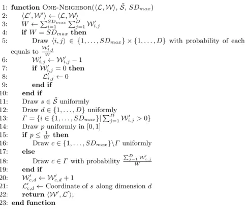
In the algorithm given in Figure 2, the model M = hL, Wi is initialized line 3 by filling all rows of the two matrices with zeros, to represent an initial empty model. The heuristic based neighborhood exploration is performed by the successive calls to function One-Neighbor() detailed in the next section. 6.3 One neighbor computation function
The function One-Neighbor() is given in Figure 3. First, it computes W the total current model weight. Then operations carried out from lines 4 to 10 de-crease the model weight when the total weight reaches the maximum model size (i.e., SDmax). This is performed by picking at random a pair of indices hi, ji with a probability proportional to Wi,j (line 5). Then the corresponding weight Wi,j is decreased (line 6). For the sake of clarity the associated coordinate Li,j is set to zero if Wi,j = 0 (line 8), even though this is not useful for the rest of the process. Next, the algorithm draws uniformly an object s in the sample
and a dimension d in the space D (lines 11 and 12). Line 13 computes the set Γ of the indices of the valid centers. Then the algorithm chooses a random center index c that corresponds either to an unused center with probability W1 (lines 15 and 16), or one of the current valid centers (line 18). In the latter case, the valid center is picked with a probability proportional to its total weight. Finally the weight Wc,d is increased and the location encoded in Lc,d is replaced by the coordinate of s along dimension d.
1: function One-Neighbor(hL, Wi, ˜S, SDmax)
2: hL0, W0i ← hL, Wi 3: W ←PSDmax i=1 PD j=1W 0 i,j 4: if W = SDmaxthen
5: Draw hi, ji ∈ {1, . . . , SDmax} × {1, . . . , D} with probability of each hi, ji
equals to W 0 i,j W 6: W0 i,j← Wi,j0 − 1 7: if Wi,j0 = 0 then 8: L0 i,j← 0 9: end if 10: end if 11: Draw s ∈ ˜S uniformly 12: Draw d ∈ {1, . . . , D} uniformly 13: Γ = {i ∈ {1, . . . , SDmax}|PDj=1Wi,j0 > 0} 14: Draw p uniformly in [0, 1] 15: if p ≤ W1 then
16: Draw c ∈ {1, . . . , SDmax}\Γ uniformly
17: else
18: Draw c ∈ Γ with probability
PD j=1Wc,j0 W 19: end if 20: Wc,d0 ← W 0 c,d+ 1 21: L0
c,d← Coordinate of s along dimension d
22: return hW0, L0i; 23: end function
Figure 3: Generation of one neighbor.
6.4 Complexity
Consider one iteration of SubCMedians using sample ˜S in a D dimensional space. Let N bCenters denote the number of centers currently used (the valid centers). Operations in non-constant time are the calls to AE, SAE and One-Neighbor(). AE computes the distance of one object to each center and is in O(N bCenters × D). SAE does the same for each object in the sample and then has a complexity O(| ˜S| × N bCenters × D). The computation cost of One-Neighbor() lies in part in the computation of weights: the total weight of the model W (line 3) and the weights in the probabilities used line 18. These values
can be maintained incrementally when W is modified resulting in a constant cost for W and in a cost proportional to N bCenters for the probabilities line 18. The remaining cost is due to the non-uniform random selections (lines 5 and 18), having a cost proportional to the number of possible outcomes. Line 5 there are at most N bCenters × D possible outcomes with a non-zero probability (other pairs hi, ji having a weight of zero). And for line 18 there are N bCenters possible outcomes. The cost of one call to One-Neighbor() is thus in O(N bCenters×D). The complexity of an iteration in SubCMedians is then O(| ˜S|×N bCenters×D). The memory requirement corresponds to the storage of the dataset S, the sample ˜S and the two matrices L and W of size SDmax× D and thus is simply in O(|S| + SDmax× D).
7
Parameter setting
The SubCMedians algorithm has three parameters: SDmax, N bIter, and N . The most important is SDmax, the maximum model size, constraining the level of detail of the subspace clustering performed. The number of iterations N bIter is also important but its setting can be avoided since the user can monitor the value of the SAE during the clustering and stop the process when this value does no longer improve. The third one, the sample size N is a way to reduce the computing resources needed, and of course if possible it makes sense to use the full dataset instead of a sample.
It this section, we propose guidelines for easy default parameter setting. In this case the only value that must be provided by the user is the expected number of clusters N bExpClust. Notice that this is not a crisp constraint, but only a suggested number of clusters that the algorithm should adjust to build a structure. Notice also that a hard part of the subspace clustering task is to determine the subspaces and that this aspect is not directly constrained by N bExpClust.
7.1 Maximum model size SDmax
The intuition to set SDmax is very simple, the value of SDmaxshould allow to build a model containing N bExpClust even if all dimensions are useful, leading to a default SDmax value equal to N bExpClust × D. Of course, as for any subspace clustering algorithm, obtaining very satisfactory results are likely to require from the user finer parameter tuning.
From N bExpClust and SDmaxwe now derive minimum recommended values for the number of iterations and for the sample size. These settings are the ones used in the experiments reported Section 9, but of course the statistical thresholds used in the setting method could be enforced in order to have more conservative recommended parameter values.
7.2 Number of iterations N bIter
Let C be any expected cluster and d be any of its dimensions. Let k be the number of attempts to set the coordinate of the center of C along d to a reasonable approximation of the median value, during N bIter iterations in SubCMedians. The default value proposed for N bIter is the minimum number of iterations such that the expected value of k is at least 1.
Let us suppose that all clusters have the same size and that the number of clusters is equal to N bExpClust. Consider an iteration of SubCMedians. In One-Neighbor() (Figure 3) the probability to pick an object s belonging to C (line 11) is 1/N bExpClust and the probability to choose dimension d (line 12) is 1/D. Let x be the coordinate of s along dimension d, and let us accept as a reasonable approximation a value x at a distance of less than 1/8 of the standard deviation away from the median. Then supposing a Gaussian distribution, this implies that the median is equal to the mean, and that the probability of x as being a reasonable approximation is about 0.1 (according to the standard normal cumulative distribution). At line 15, the probability to jump to line 18 to modify an existing cluster is 1 − 1/W . If we suppose that the current model contains already N bExpClust clusters, including C (possibly with the presence of a single dimension of C), and that all clusters have similar weights in matrix W, then the probability of C to be chosen in line 18 is about 1/N bExpClust. So the probability p of the center corresponding to C in the current model, to have its coordinate along dimension d to be set to a reasonable approximation x in line 21, is p = N bExpClust1 × 1 D× 0.1 × (1 − 1 W) × 1 N bExpClust. As W increases at each iteration (up to SDmax) we quickly have (1 −W1) ' 1, and since we set SDmax= N bExpClust × D, we have p ' 0.1 × SD 1
max×N bExpClust.
The expected value of k is E(k) = N bIter × p, thus to have E(k) ≥ 1, the default minimum N bIter value is set to 10 × SDmax× N bExpClust.
7.3 Dataset sample size N
Consider a cluster C and a dimension d, supposing that the coordinates in C along d follow N (µd, σd). As stated in Section 5.2, ˆθd the median estimator of these coordinates, using a sample of size n, follows N (µd, σd
pπ
2n). If we accept a standard error of 1/4 of the original σdthen the minimum sample size satisfies σθˆ
d = σd
4 = σd pπ
2n and we have n = 8π ' 25. Such sample allows to estimate the median location of a cluster in the D dimensions, but if there are N bExpClust clusters, more objects are needed. Let us suppose that all clusters have the same size, and thus are likely to be represented by similar numbers of objects in the sample, then the recommended minimum value for N is 25 × N bExpClust.
8
Experimental setup
8.1 Experimental protocol
The SubCMedians algorithm extends the subspace clustering tool family towards medians based clustering. Even if cluster center locations based on medians can
be interesting on their own (depending on the targeted task), an open question is to what extent the quality of the clusters obtained competes with those given by other paradigms? In order to evaluate and compare SubCMedians with the state-of-the-art approaches we used the evaluation framework of reference de-signed for subspace clustering described in [9]. This evaluation framework relies on a systematic approach to compare the results of representative algorithms that address the major subspace clustering paradigms. The comparison detailed in [9] was made using different evaluation measures on both real and synthetic datasets, using the following method. Given that each algorithm requires several parameters (from 2 to 9), for each dataset, the algorithms were executed with 100 different parameter settings to explore the parameter space. Then, using an external labeling of the objects, only the outputs that were among the best with respect to the external labeling (taken as a ground truth) were retained. So, the results reported in [9] are in some sense the best possible subspace clusterings that could be achieved if we were able to find the most appropriate parameter values. More precisely, for each real world dataset only two outputs were retained: 1) the one computed for the parameter setting that maximizes the F1measure, and 2) the one obtained when maximizing the accuracy. These two outputs led to two values for each measure, the smallest of the two being called bestMin and the other bestMax. For each synthetic dataset, all the settings maximizing at least one quality measures among F1, accuracy, CE, RN IA and entropy were retained.
Since generally no external labeling is available when we search for clusters, parameter tuning is most of the time a difficult task and these high quality subspace clustering models are likely to be hard to obtain. Here, for SubCMedi-ans, the parameters were not optimized using any external criteria. Instead the parameters were set using the default values suggested in Section 7. Thus, we compare clusterings effectively found by SubCMedians to the best clusterings that could potentially be found by the other algorithms. Since SubCMedians is nondeterministic (as many subspace clustering approaches), it can achieve different results on different runs. Consequently the algorithm was executed 10 times independently using the same parameter setting. The results obtained af-ter each run were assessed with the same criaf-teria as in [9]: the coverage, the number of clusters found, different quality measures (F1, accuracy, CE, RN IA and entropy) and the runtime. For each real world dataset, the highest and lowest values of each evaluation measure (over the 10 runs) were computed, so as to compare with the bestMin and bestMax values retained by the evaluation method of [9]. For each synthetic dataset, we simply took the clustering having the lowest SAE measure (internal criterion of quality).
In addition, to assess the impact of the weighted neighborhood exploration of the model space used by SubCMedians, the algorithm was compared to an unweighted version, in which the candidate center undergoing the modification is uniformly drawn. More precisely, the candidate center is uniformly drawn among the SDmaxpotential candidate centers that could be contained in a model of size SDmax. This version was obtained by changing lines 15 to 19 of the algorithm
given in Figure 3, and replacing line 20 by Wc,d0 ← 1, to have matrices W0 and W containing simply a 1 for a dimension that is used and a 0 otherwise.
All experiments were run on an Intel 2.67GHz CPU running Linux Debian 8.3, using a single core and less than 150 MB of RAM. The SubCMedians algo-rithm has been implemented in C++ as a Python library and in Java as a Knime component. The reported runtimes are the ones obtained with the C++/Python version.
8.2 Datasets
The performances of SubCMedians are reported on real world data using the seven benchmark datasets selected in [9] for their representativity: breast, dia-betes, liver, glass, shape, pendigits and vowel (most of them coming from the UCI archive [2]). These datasets have different dimensionalities and contain different numbers of objects. These objects are already structured in classes, and the class membership is used by quality measures to assess the cluster purity. However, the number of classes does not necessarily reflect the number of subspace clus-ters, and the objects of a class can form different groups in space and/or strongly overlap with the objects of other classes.
SubCMedians was also executed on the 16 synthetic benchmark datasets provided by [9]. These datasets are particularly useful to study the algorithm performances, as the true clusters and their subspaces are known. Each dataset contains 10 hidden subspace clusters laying in subspaces made by 50%, 60% and 80% of the total dimensions of the dataset. Seven synthetic datasets allow to study scalability with respect to the dataset dimensionality (5, 10, 15, 20, 25, 50 and 75 dimensions). These datasets contain about 1500 objects each and are extended with about 10% of noise objects. Five other synthetic datasets permit to analyse the scalability with respect to the dataset size (1500, 2500, 3500, 4500 and 5500 objects), over 20 dimensions and also with about 10% of noise objects. Finally four datasets allow to study the capacity to cope with noise, containing 10%, 30%, 50% and up to 70% of noise objects.
All datasets are made available by the authors of [9] at http://dme.rwth-aachen.de/openSubspace/evaluation. We applied a z-score standardization to all real and synthetic datasets in a preprocessing step.
8.3 Parameter values
SubCMedians parameters were set according to Section 7. Let D denote the dimensionality of each particular dataset. For the synthetic datasets the num-ber of expected clusters is about 10, thus the maximum model size was set to SDmax = D × 10, the sample size was set to N = 25 × 10 and the number of iterations was set to N bIter = 10 × 10 × SDmax. A weaker setting, not based on the true number of clusters, but based on 20 expected clusters, was also used, and as reported in Section 9 still permitted to exhibit structures of about 10 clusters. For the real world datasets, the only information available
about the structure of the datasets is the number of classes. However, as al-ready mentioned, the number of classes may not correspond to the number of clusters. Indeed, according to the results provided by [9], in these datasets the state-of-the-art algorithms exhibit most of the time structures composed of more clusters than the number of classes. The setting of SubCMedians parameters is thus based on an expected number of clusters equal to three times the number of classes and we let the algorithm regulate itself the number of output clusters. Hence the maximum model size was set to SDmax = 3 × N bClasses × D, the sample size was set to N = 25 × 3 × N bClasses and the number of iterations was set to N bIter = 10 × 3 × N bClasses × SDmax.
8.4 Evaluation measures
In order to compare our algorithm to the others, we used the same standard evaluation measures for clusters and subspace clusters as [9]: entropy (the nor-malized entropy), accuracy, F 1, RN IA and CE. We performed also the same simple transformation on entropy and RN IA, by computing RN IA = 1−RN IA and entropy = 1 − entropy to have all evaluation measures ranging from 0 (low quality) to 1 (high quality). The three first measures (entropy, accuracy and F 1) reflect how well objects that should have been grouped together were effectively grouped. The two last measures (RN IA and CE) take into account the way the objects are grouped and also the relevance of the subspaces found by the algo-rithm. For these measures, when the true dimensions of the subspace clusters were not known (for real datasets), then as in [9] all dimensions were considered as relevant, but then the interpretation of these two measures should remain cautious since the true sets of dimensions are likely to be smaller. Of course this does not apply to the synthetic datasets, since for them the reference clusters and their dimensions are known. We refer the reader to [9] for the detailed recall of the evaluation measures.
9
Experimental results
Because of the large number of results (23 datasets and 11 algorithms) used in the comparison, aggregated figures reflecting the real detailed results are given. However, there is no ever winning paradigm or clustering method, each having its own advantages or interest. The main objective of this section is to provide evidences to investigate the two following questions: Are subspace clusters based on medians comparable to results obtained by state-of-the-art approaches? Is SubCMedians an effective method for such a clustering?
9.1 Real dataset
This section presents the results obtained on the 7 representative real datasets selected in [9] using the following aggregations.
Cluster quality measures For each measure, on each data set, two rankings of the 11 algorithms were computed: one for the bestM ax score and one for the bestM in score, with ranks ranging from 1 to 11, rank 11 being associated to the algorithm obtaining the highest quality. The overall ranking of an algorithm was then simply the average of its rank values.
Runtimes The same ranking was used to compare the algorithm using the run-time measure, associating rank value 11 to the fastest. Even if SubCMedians and Chameleoclust+ have been executed on a computer (2.67GHz CPU) differ-ent from the one used by [9] (2.3GHz CPU), we report the runtimes comparison, since at least the orders of magnitude can still be meaningful.
Coverage The same procedure was used to compare the coverages obtained. The coverage denotes the fraction of objects of the dataset that are associated to clusters. This measure is less than 1 if some objects are not associated to one of the output clusters, or if they are identified as outliers or as reflecting noise. When the coverage decreases, discarding some objects can result in a direct improvement of several quality measures (because of clusters being more homogeneous). Of course putting apart too many objects is likely to lead to less representative models and is most of the time not desirable. For the coverage a rank value of 11 was associated to the highest coverage.
Number of clusters The rankings were computed using the absolute value of the difference between the number of clusters found by the algorithm and the number of classes in the dataset. The rank value 11 is given to the smallest absolute value. However, as previously mentioned, the number of classes does not necessarily reflect the number of subspace clusters in the datasets.
The global trade-off is then to reach high quality measures while preserving a high coverage (except for data containing many outliers or important noise), and without splitting the data into too many clusters.
The average rank of each algorithm regarding the cluster quality measures, the runtime, the coverage and the number of clusters found are given in Figure 4. In addition, the results on the real world datasets are presented in Figure 5. These tables report on the seven real world datasets, for the 10 state-of-the-art algorithms, Chameleoclust+ and SubCMedians the bestM in and bestM ax values for the different quality measures, the coverage, the number of clusters found, their average dimensionality and the runtimes. According to these results SubCMedians is faster than Chameleoclust+ and usually outputs results with higher quality.
Figure 4 shows evidence that the robustness of the medians still operates in a subspace clustering task since competitive cluster qualities can be obtained with-out discarding any object (100% coverage). SubCMedians was able to find these clusterings in short execution times, and using an effective parameter setting (no parameter optimization using an external ground truth). For the number of clusters found, SubCMedians is above the average, and it seems that it does not
tend to split the dataset into too many clusters. However, the true numbers of clusters are not known here, in contrast to the synthetic datasets.
1 2 3 4 5 6 7 8 9 10 11 12
Averagequalityrank
MINECLUS SUBCMEDIANS DOC PROCLUS INSCY STATPC P3C SCHISM CLIQUE SUBCLU FIRES 1 2 3 4 5 6 7 8 9 10 11 12
Averageruntimerank
SUBCMEDIANS FIRES PROCLUS P3C CLIQUE SCHISM SUBCLU MINECLUS STATPC INSCY DOC 1 2 3 4 5 6 7 8 9 10 11 12
Averagecoveragerank
SUBCMEDIANS CLIQUE SUBCLU MINECLUS SCHISM DOC P3C STATPC INSCY PROCLUS FIRES 1 2 3 4 5 6 7 8 9 10 11 12
AverageNbClustersrank
P3C FIRES PROCLUS SUBCMEDIANS DOC STATPC MINECLUS INSCY SUBCLU SCHISM CLIQUE
Figure 4: Average rankings over all datasets regarding the quality, the runtime, the coverage and the number of clusters.
9.2 Synthetic data
In this section, we report the results obtained on the 16 synthetic datasets of [9], each one containing 10 known clusters. For each dataset, SubCMedians was ex-ecuted 10 times and the model having the lowest SAE was retained (no use of external labeling). These models are depicted as red circles in Figure 6. The green shapes represent the areas where are located the best models found by the 10 other algorithms over their parameter spaces (optimized using external ground truth labeling). Here again, the results show evidences that a median based approach is an interesting complementary tool for subspace clustering, and in particular that SubCMedians reaches a competitive quality for the measures that take into account not only the objects grouping, but also the dimensions associated to the clusters (RN IA and CE). In these experiments the parame-ters where computed according to the guidelines of Section 7 using an expected number of clusters of 10, but no constraint on the sizes of their subspaces. In-terestingly, a weaker setting based on an expected number of clusters of 20 still permits to SubCMedians to exhibit most of the time a good quality clustering of about 10 clusters (e.g., RN IA and Accuracy in Figure 7).
The results of the more naïve unweighted version of SubCMedians are rep-resented in Figure 6 by blue triangles (same procedure used, retaining also the
DATASET: F 1 Accuracy CE RN IA Entropy Coverage N umClusters AvgDim Runtime BREAST max min max min max min max min max min max min max min max min max min
CLIQUE 0.67 0.67 0.71 0.71 0.02 0.02 0.40 0.40 0.26 0.26 1.00 1.00 107 107 1.7 1.7 453 453 DOC 0.73 0.61 0.81 0.76 0.11 0.04 0.84 0.07 0.46 0.27 1.00 0.80 60 6 27.2 2.8 1E+06 37515 MINECLUS 0.78 0.69 0.78 0.76 0.19 0.18 1.00 1.00 0.56 0.37 1.00 1.00 64 32 33.0 33.0 40359 29437 SCHISM 0.67 0.67 0.75 0.69 0.01 0.01 0.36 0.34 0.35 0.34 1.00 0.99 248 197 2.3 2.2 158749 114609 SUBCLU 0.68 0.51 0.77 0.67 0.02 0.01 0.54 0.04 0.27 0.24 1.00 0.82 357 5 2.0 1.0 5265 16 FIRES 0.49 0.03 0.76 0.76 0.03 0.00 0.05 0.00 1.00 0.01 0.76 0.04 11 1 2.5 1.0 250 31 INSCY 0.74 0.55 0.77 0.76 0.02 0.00 0.24 0.11 0.60 0.39 0.97 0.74 2038 167 11.0 4.4 134373 63484 PROCLUS 0.57 0.52 0.80 0.74 0.51 0.11 0.65 0.43 0.32 0.23 0.89 0.69 9 2 24.0 18.0 703 141 P3C 0.63 0.63 0.77 0.77 0.04 0.04 0.19 0.19 0.36 0.36 0.85 0.85 28 28 6.9 6.9 6281 6281 STATPC 0.41 0.41 0.78 0.78 0.16 0.16 0.33 0.33 0.29 0.29 0.43 0.43 5 5 33.0 33.0 5187 4906 CHAMELEOCLUST+ 0.60 0.51 0.76 0.76 0.23 0.11 0.53 0.25 0.25 0.22 1 1 8 4 16.75 5.75 339 131 SUBCMEDIANS 0.66 0.57 0.79 0.76 0.18 0.14 0.56 0.51 0.31 0.25 1 1 19.0 13.0 12.36 9.26 8 7
DATASET: F 1 Accuracy CE RN IA Entropy Coverage N umClusters AvgDim Runtime PENDIGITS max min max min max min max min max min max min max min max min max min
CLIQUE 0.30 0.17 0.96 0.86 0.06 0.01 0.20 0.06 0.41 0.26 1.00 1.00 1890 36 3.1 1.5 67891 219 DOC 0.52 0.52 0.54 0.54 0.18 0.18 0.35 0.35 0.53 0.53 0.91 0.91 15 15 5.5 5.5 178358 178358 MINECLUS 0.87 0.87 0.86 0.86 0.48 0.48 0.89 0.89 0.82 0.82 1.00 1.00 64 64 12.1 12.1 780167 692651 SCHISM 0.45 0.26 0.93 0.71 0.05 0.01 0.30 0.08 0.50 0.45 1.00 0.93 1092 290 10.1 3.4 5E+08 21266 SUBCLU - - - -FIRES 0.45 0.45 0.73 0.73 0.09 0.09 0.33 0.33 0.31 0.31 0.94 0.94 27 27 2.5 2.5 169999 169999 INSCY 0.65 0.48 0.78 0.68 0.07 0.07 0.30 0.28 0.77 0.69 0.91 0.82 262 106 5.3 4.6 2E+06 1E+06 PROCLUS 0.78 0.73 0.74 0.73 0.31 0.27 0.64 0.45 0.90 0.71 0.90 0.74 37 17 14.0 8.0 6045 4250
P3C 0.74 0.74 0.72 0.72 0.28 0.28 0.58 0.58 0.76 0.76 0.90 0.90 31 31 9.0 9.0 2E+06 2E+06 STATPC 0.91 0.32 0.92 0.10 0.09 0.00 0.67 0.11 1.00 0.53 0.99 0.84 4109 56 16.0 16.0 5E+07 3E+06 CHAMELEOCLUST+0.71 0.51 0.74 0.59 0.51 0.30 0.78 0.49 0.68 0.58 1 1 14 10 12.40 7.21 4476 4226
SUBCMEDIANS 0.92 0.89 0.92 0.89 0.40 0.34 0.80 0.78 0.89 0.86 1 1 41.0 34.0 12.21 10.51 556 523 DATASET: F 1 Accuracy CE RN IA Entropy Coverage N umClusters AvgDim Runtime DIABETES max min max min max min max min max min max min max min max min max min
CLIQUE 0.70 0.39 0.72 0.69 0.03 0.01 0.14 0.01 0.23 0.13 1.00 1.00 349 202 4.2 2.4 11953 203 DOC 0.71 0.71 0.72 0.69 0.31 0.26 0.92 0.79 0.31 0.24 1.00 0.93 64 17 8.0 5.1 1E+06 51640 MINECLUS 0.72 0.66 0.71 0.69 0.63 0.13 0.89 0.58 0.29 0.17 0.99 0.96 39 3 6.0 5.2 3578 62 SCHISM 0.70 0.62 0.73 0.68 0.08 0.01 0.36 0.09 0.34 0.20 1.00 0.79 270 21 4.2 3.9 35468 250 SUBCLU 0.74 0.45 0.71 0.68 0.01 0.01 0.01 0.01 0.14 0.11 1.00 1.00 1601 325 4.7 4.0 190122 58718 FIRES 0.52 0.03 0.65 0.64 0.12 0.00 0.27 0.00 0.68 0.00 0.81 0.03 17 1 2.5 1.0 4234 360 INSCY 0.65 0.39 0.70 0.65 0.37 0.11 0.45 0.42 0.44 0.15 0.83 0.73 132 3 6.7 5.7 112093 33531 PROCLUS 0.67 0.61 0.72 0.71 0.34 0.21 0.78 0.69 0.23 0.19 0.92 0.78 9 3 8.0 6.0 360 109 P3C 0.39 0.39 0.66 0.65 0.56 0.11 0.85 0.22 0.09 0.07 0.97 0.88 2 1 7.0 2.0 656 141 STATPC 0.73 0.59 0.70 0.65 0.06 0.00 0.63 0.17 0.72 0.28 0.97 0.75 363 27 8.0 8.0 27749 4657 CHAMELEOCLUST+ 0.70 0.62 0.73 0.70 0.17 0.09 0.66 0.47 0.28 0.23 1 1 29 19 5.00 2.75 598 438 SUBCMEDIANS 0.69 0.64 0.73 0.70 0.21 0.08 0.55 0.40 0.25 0.21 1 1 16.0 13.0 3.69 2.87 3 3
DATASET: F 1 Accuracy CE RN IA Entropy Coverage N umClusters AvgDim Runtime GLASS max min max min max min max min max min max min max min max min max min CLIQUE 0.51 0.31 0.67 0.50 0.02 0.00 0.06 0.00 0.39 0.24 1.00 1.00 6169 175 5.4 3.1 411195 1375 DOC 0.74 0.50 0.63 0.50 0.23 0.13 0.93 0.33 0.72 0.50 0.93 0.91 64 11 9.0 3.3 23172 78 MINECLUS 0.76 0.40 0.52 0.50 0.24 0.19 0.78 0.45 0.72 0.46 1.00 0.87 64 6 7.0 4.3 907 15 SCHISM 0.46 0.39 0.63 0.47 0.11 0.04 0.33 0.20 0.44 0.38 1.00 0.79 158 30 3.9 2.1 313 31 SUBCLU 0.50 0.45 0.65 0.46 0.00 0.00 0.01 0.01 0.42 0.39 1.00 1.00 1648 831 4.9 4.3 14410 4250 FIRES 0.30 0.30 0.49 0.49 0.21 0.21 0.45 0.45 0.40 0.40 0.86 0.86 7 7 2.7 2.7 78 78 INSCY 0.57 0.41 0.65 0.47 0.23 0.09 0.54 0.26 0.67 0.47 0.86 0.79 72 30 5.9 2.7 4703 578 PROCLUS 0.60 0.56 0.60 0.57 0.13 0.05 0.51 0.17 0.76 0.68 0.79 0.57 29 26 8.0 2.0 375 250 P3C 0.28 0.23 0.47 0.39 0.14 0.13 0.30 0.27 0.43 0.38 0.89 0.81 3 2 3.0 3.0 32 31 STATPC 0.75 0.40 0.49 0.36 0.19 0.05 0.67 0.37 0.88 0.36 0.93 0.80 106 27 9.0 9.0 1265 390 CHAMELEOCLUST+ 0.43 0.28 0.57 0.50 0.43 0.26 0.88 0.55 0.46 0.36 1 1 8 4 7.50 4.75 195 95 SUBCMEDIANS 0.65 0.51 0.71 0.60 0.32 0.24 0.85 0.76 0.64 0.55 1 1 23.0 19.0 6.74 5.7 18 16 DATASET: F 1 Accuracy CE RN IA Entropy Coverage N umClusters AvgDim Runtime LIVER max min max min max min max min max min max min max min max min max min CLIQUE 0.68 0.65 0.67 0.58 0.08 0.02 0.38 0.03 0.10 0.02 1.00 1.00 1922 19 4.1 1.7 38281 15 DOC 0.67 0.64 0.68 0.58 0.11 0.07 0.51 0.35 0.18 0.11 0.99 0.90 45 13 3.0 1.9 625324 1625 MINECLUS 0.73 0.63 0.65 0.58 0.09 0.09 0.68 0.48 0.33 0.16 0.99 0.92 64 32 4.0 3.7 49563 1954 SCHISM 0.69 0.69 0.68 0.59 0.04 0.03 0.45 0.26 0.10 0.08 0.99 0.99 90 68 2.7 2.1 31 0 SUBCLU 0.68 0.68 0.64 0.58 0.11 0.02 0.68 0.05 0.07 0.02 1.00 1.00 334 64 3.4 1.3 1422 47 FIRES 0.58 0.04 0.58 0.56 0.14 0.00 0.39 0.01 0.37 0.00 0.84 0.03 10 1 3.0 1.0 531 46 INSCY 0.66 0.66 0.62 0.61 0.03 0.03 0.42 0.39 0.21 0.20 0.85 0.81 166 130 2.1 2.1 407 234 PROCLUS 0.53 0.39 0.63 0.63 0.26 0.11 0.66 0.25 0.05 0.05 0.83 0.46 6 2 5.0 3.0 78 31 P3C 0.36 0.35 0.58 0.58 0.55 0.27 0.96 0.47 0.02 0.01 0.98 0.94 2 1 6.0 3.0 172 32 STATPC 0.69 0.57 0.65 0.58 0.23 0.01 0.58 0.37 0.63 0.05 0.77 0.71 159 4 6.0 3.3 1890 781 CHAMELEOCLUST+0.65 0.59 0.68 0.62 0.20 0.10 0.53 0.41 0.14 0.07 1 1 27 22 2.48 1.85 202 158 SUBCMEDIANS 0.65 0.56 0.67 0.60 0.21 0.09 0.56 0.43 0.12 0.04 1 1 17.0 11.0 2.82 2.0 2 2 DATASET: F 1 Accuracy CE RN IA Entropy Coverage N umClusters AvgDim Runtime SHAPE max min max min max min max min max min max min max min max min max min CLIQUE 0.31 0.31 0.76 0.76 0.01 0.01 0.07 0.07 0.66 0.66 1.00 1.00 486 486 3.3 3.3 235 235 DOC 0.90 0.83 0.79 0.54 0.56 0.38 0.90 0.82 0.93 0.86 1.00 1.00 53 29 13.8 12.8 2E+06 86500 MINECLUS 0.94 0.86 0.79 0.60 0.58 0.46 1.00 1.00 0.93 0.82 1.00 1.00 64 32 17.0 17.0 46703 3266 SCHISM 0.51 0.30 0.74 0.49 0.10 0.00 0.26 0.01 0.85 0.55 1.00 0.92 8835 90 6.0 3.9 712964 9031 SUBCLU 0.36 0.29 0.70 0.64 0.00 0.00 0.05 0.04 0.89 0.88 1.00 1.00 3468 3337 4.5 4.1 4063 1891 FIRES 0.36 0.36 0.51 0.44 0.20 0.13 0.25 0.20 0.88 0.82 0.45 0.39 10 5 7.6 5.3 63 47 INSCY 0.84 0.59 0.76 0.48 0.18 0.16 0.37 0.24 0.94 0.87 0.88 0.82 185 48 9.8 9.5 22578 11531 PROCLUS 0.84 0.81 0.72 0.71 0.25 0.18 0.61 0.37 0.93 0.91 0.89 0.79 34 34 13.0 7.0 593 469 P3C 0.51 0.51 0.61 0.61 0.14 0.14 0.17 0.17 0.80 0.80 0.66 0.66 9 9 4.1 4.1 140 140 STATPC 0.43 0.43 0.74 0.74 0.45 0.45 0.55 0.55 0.56 0.56 0.92 0.92 9 9 17.0 17.0 250 171 CHAMELEOCLUST+ 0.75 0.63 0.80 0.71 0.54 0.49 0.78 0.71 0.77 0.67 1 1 14 10 12.40 10.79 462 252 SUBCMEDIANS 0.82 0.72 0.86 0.79 0.57 0.53 0.86 0.80 0.83 0.77 1 1 19.0 16.0 13.5 12.56 101 91 DATASET: F 1 Accuracy CE RN IA Entropy Coverage N umClusters AvgDim Runtime
VOWEL max min max min max min max min max min max min max min max min max min CLIQUE 0.23 0.17 0.64 0.37 0.05 0.00 0.44 0.01 0.10 0.09 1.00 1.00 3062 267 4.9 1.9 523233 1953 DOC 0.49 0.49 0.44 0.44 0.14 0.14 0.85 0.85 0.58 0.58 0.86 0.86 64 64 10.0 10.0 120015 120015 MINECLUS 0.48 0.43 0.37 0.37 0.09 0.04 0.62 0.34 0.60 0.46 0.98 0.87 64 64 7.2 3.6 7734 5204 SCHISM 0.37 0.23 0.62 0.52 0.05 0.01 0.43 0.11 0.29 0.21 1.00 0.93 494 121 4.3 2.8 23031 391 SUBCLU 0.24 0.18 0.58 0.38 0.04 0.01 0.39 0.04 0.30 0.13 1.00 1.00 10881 709 3.6 2.0 26047 2250 FIRES 0.16 0.14 0.13 0.11 0.02 0.02 0.14 0.13 0.16 0.13 0.50 0.45 32 24 2.1 1.9 563 250 INSCY 0.82 0.33 0.61 0.15 0.09 0.07 0.75 0.26 0.94 0.21 0.90 0.81 163 74 9.5 4.3 75706 39390 PROCLUS 0.49 0.49 0.44 0.44 0.11 0.11 0.53 0.53 0.65 0.65 0.67 0.67 64 64 8.0 8.0 766 766 P3C 0.08 0.05 0.17 0.16 0.12 0.08 0.69 0.43 0.13 0.12 0.98 0.95 3 2 7.0 4.7 1610 625 STATPC 0.22 0.22 0.56 0.56 0.06 0.06 0.12 0.12 0.14 0.14 1.00 1.00 39 39 10.0 10.0 18485 16671 CHAMELEOCLUST+ 0.41 0.37 0.42 0.38 0.17 0.13 0.65 0.54 0.45 0.40 1 1 33 24 6.00 4.57 995 787 SUBCMEDIANS 0.53 0.48 0.53 0.47 0.16 0.14 0.75 0.70 0.56 0.52 1 1 50.0 45.0 6.82 6.3 364 339
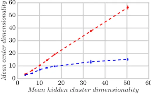
lowest SAE over 10 runs). The unweighted-SubCMedians outputted slightly more clusters than expected, and has another more important drawback, that is the lower quality obtained with respect to the dimensions found (RN IA and CE graphics). As targeted by the design of the neighborhood exploration in Sec-tion 6, the weighted strategy of SubCMedians could focus on more promising clusters while unweighted-SubCMedians produced more (useless) candidate centers (Figure 8) and failed to develop sufficiently the center dimensionalities when the hidden cluster dimensionalities increased (Figure 9). Moreover, SubCMedi-ans turned out to be slightly faster (see Figures 10 and 11), and unweighted-SubCMedians suffered from a small overhead likely to be caused by its handling of more candidate centers in the models.
1 10 100 1000 10000 Numberofclusters 0.0 0.1 0.2 0.3 0.4 0.5 0.6 0.7 0.8 0.9 1.0
A
cc
ur
ac
y
1 10 100 1000 10000 Numberofclusters 0.0 0.1 0.2 0.3 0.4 0.5 0.6 0.7 0.8 0.9 1.0F
1 1 10 100 1000 10000 Numberofclusters 0.0 0.1 0.2 0.3 0.4 0.5 0.6 0.7 0.8 0.9 1.0En
tr
op
y
1 10 100 1000 10000 Numberofclusters 0.0 0.1 0.2 0.3 0.4 0.5 0.6 0.7 0.8 0.9 1.0CE
1 10 100 1000 10000 Numberofclusters 0.0 0.1 0.2 0.3 0.4 0.5 0.6 0.7 0.8 0.9 1.0R
N
IA
Figure 6: Quality measures and number of clusters obtained on synthetic datasets by SubCMedians (red circles), unweighted-SubCMedians (blue triangles) and the other algorithms (green areas).
1 10 100 1000 10000 Numberofclusters 0.0 0.1 0.2 0.3 0.4 0.5 0.6 0.7 0.8 0.9 1.0
R
N
IA
1 10 100 1000 10000 Numberofclusters 0.0 0.1 0.2 0.3 0.4 0.5 0.6 0.7 0.8 0.9 1.0A
cc
ur
ac
y
Figure 7: RN IA and Accuracy vs number of clusters obtained on synthetic datasets by SubCMedians under weaker parameter setting (black stars).
0 10 20 30 40 50 60 70 80 Datasetdimensionality 0 50 100 150 200 250 300 350 400
N
um
be
r
of
ca
nd
id
at
e
ce
nt
er
s
Figure 8: Number of candidate centers (avg. 10 runs) for SubCMedians (red cir-cles) and unweighted-SubCMedians (blue triangles) vs dataset dimensionality.
10
EvoMove system
In the EvoMove system (Figure 1), SubCMedians is used as the move recognition algorithm. In the first part of this section, we give more details about EvoMove, and in particular we describe what are the input and output of SubCMedians in this system. During the prototyping and tests of EvoMove, we had the occasion to work with professional dancers to go deeper in our understanding of what is happening in the system and to which extend it could be used and enhanced. Two short videos of this exploration are given as supplementary material to this report (EvoMove AnouSkan 1 https://www.youtube.com/watch?v=p_eJFiQfW1E and EvoMove AnouSkan 2 https://www.youtube.com/watch?v=E85B1jJOiBQ). In this section we also comment on some typical behaviors of the system, and give some insight on how users perceived the system and their interaction with it.
0 10 20 30 40 50 60
Meanhiddenclusterdimensionality
0 10 20 30 40 50 60
M
ea
n
ce
nt
er
di
m
en
si
on
al
ity
Figure 9: Subspace mean size of the centers (avg. 10 runs) for SubCMedians (red circles) and unweighted-SubCMedians (blue triangles) vs subspace mean size of the hidden clusters.
0 500 1000 1500 Samplesize 0.1 1 10 100 1000
R
un
tim
e
(
se
co
nd
s
)
Figure 10: Runtimes (avg. 10 runs) for SubCMedians (red circles) and unweighted-SubCMedians (blue triangles) vs sample sizes (| ˜S|) for the synthetic dataset of size 5500. 5 10 15 20 25 50 75 Datasetdimensionality 0.1 1 10 100 1000
R
un
tim
e
(
se
co
nd
s
)
Figure 11: Runtimes (avg. 10 runs) for SubCMedians (red circles) and unweighted-SubCMedians (blue triangles) vs synthetic dataset dimensionalities.
10.1 Description of the system
At the beginning of each session, the set of available audio samples and the num-ber of sensors, as well as a few options are chosen, and then a new instance of SubCMedians is launched. Each sensor is an Inertial Measurement Unit (IMU) composed of three orthogonal accelerometers, three orthogonal gyroscopes mea-suring angular speed, and three orthogonal magnetometers. They are embedded in small black boxes visible tight to the wrists of the dancers in the videos. Each IMU is delivering information at 50 Hz, that is collected by a gateway compo-nent. This information is aggregated every time step. This adjustable time step is set to correspond to a beat of the played music. For instance, if the tempo is set to 60 bpm, as in the videos, the time step will be one-second long. At the end of each time step, the mean and variance of the 9 measures (3 accelerations, 3 angular speeds, 3 magnetic field measures) collected during this time step are computed. Computing these means and variances of the 9 measures leads to 18 values to describe the move that occurs during the time step, and forms a data point in a space having 18 dimensions. This data point is then sent as input to the SubCMedians instance associated to the session. So, each time step corre-sponds to a point in a data stream that is clusterized by SubCMedians, where each cluster contains data points corresponding to a similar move. In the videos, the instance of SubCMedians uses a value of 100 for parameter SDmax, a sliding window containing 100 data points (size of data sample), and performs a local exploration in the model space using 100 neighbors each time the sliding window is updated.
After the acquisition of a new data point P , EvoMove determines the group of moves the most similar to P by finding the cluster center that is the closest to P , and sets a trigger to start to play (on the next beat) the audio sample associated to this cluster identifier. The sliding window is then updated (P is added to the window and the oldest point in the window is removed). And next, SubCMedians performs a local exploration of the neighborhood of the current clustering model, to try to build a better clustering using the updated window. From the user perspective, if the tempo is set to 60 bpm (as for instance in the two videos), this means that every second a description of the user move is computed, an audio sample is started, and the system adapts its clustering model.
Beyond the preprocessing (computing means and variances over one time step), and the SubCMedians settings, the interaction can be influenced by several other parameters. Here are the ones used in the sessions recorded on the videos: – When does an audio sample start ? At the end of a time step the user move made during this time step is associated to a cluster identifier that is mapped to the audio sample to be played. This sample started to be played on the next beat.
– What is the duration of an audio sample ? The used samples have a duration ranging from one time step up to four time steps (most of them spreading over four time steps). When samples are longer than one time step, then a
sample can be started while the previous one is not finished, and thus the sound of both can be superimpose. This results in several samples (up to four) being superimposed at some time steps. This gives a feeling of "trails", moves initiating sounds that will fully stop later. Notice the following particular case: If it is the same sample that is started while it was already being played then it is not superimposed onto itself, and its ongoing playback is stopped, while a new playback of it is started.
– How many instances of SubCMedians are used at the same time ? In the videos, dancers are equipped with two sensors and two different instances of SubCMedians are running, each one processing the data points coming from one of the sensor and using its own set of audio samples.
This detailed setup is only one of the numerous possible ones with this system. For instance, several users could wear sensors, several sensor measures could be combined to describe moves (e.g., using the difference between two measures or their product). And of course, different audio samples could be used, including samples that could be modified during a session over time such as in preliminary experiments we have presented in [1].
10.2 User perception and system behavior
Several questions motivated the EvoMove demonstrator. Besides questions about the efficiency of the technology, we wondered what it would be like to interact with this system. Does the user has the feeling of an interaction ? Does it seem to her/him that the system behaves randomly or that she/he influences the system in some directions ?
During the development of the project, we had the occasion to organize trial sessions with different users. During these sessions we also ask them about their feeling about the system and their interaction with it. These tests were per-formed with people having different backgrounds and different approaches of the system, ranging from people that were the developers of the project them-selves, to professional dancers and also musicians. From the discussions we had with these different users, it appeared that they had very distinct representa-tions of what the system was doing. In particular they imagined very different usages/applications of the system, ranging from its use as a dance improvisation companion to its use as an electronic instrument that could be master to control what sound will be played by the system and when.
It turned out that the users also thought/spoke about the system in very different ways. Here are three examples of these mental representations and feeeling about the interactions: (The descriptions given here have been collected from different users after their first trial of the system)
– A musician: Felt like being involved in a teaching relationship with the sys-tem, trying to repeat gestures so as for the machine to memorize it, trying to insist on some distinctions between gestures, etc, as if she/he were teaching a trick to an animal.
– A dancer: Perceived the system as a good monitoring tool for her moves, that was noticing small move differences by playing a different sound, as if a specialist (a dance teacher) were checking the correctness of her moves. – One of the developers of the system: As the system is based on a clustering
algorithm dealing with sets of points and subspaces, he thought about it in a geometrical way. His perception, when using the system, is to be placing points in a multidimensional space, so as to push and pull candidate cluster centers around in this space.
These really different representations illustrate the wide scope of applications of this EvoEvo technology. Moreover, some emergent behaviors of the systems we did not predict seems really interesting. Let us illustrate two examples of this behaviors on the video EvoMove AnouSkan 1.
Concept drift In nature, evolution does not happen in a static world, but in an evolving one. Thus, organisms have to constantly adapt there existing functions to new environments. For instance, predators have to adapt their weapons (teeth, claws, etc) to their co-evolving preys. In the EvoMove system, functions are clusters. A new cluster appears when a new move is introduced by the user. But the user could also decide to modify a bit one of her/his moves. Thanks to its adaptable nature the system is able to follow this modification. An example of this behavior is really clear in the video EvoMove AnouSkan 1, from timestamp 1’28 to 1’54 where we can see the dancer slightly transforming her moves at each repetition, while the sound remains the same. As each audio sample corresponds to a cluster, we know that the same cluster is used all along these thirty seconds, but has been drift in the clustering space by the system, following the gradual changes of the move made by the dancer when repeating it.
Seasonality Some proteins are specific to a situation, or environment to which living organisms could be confronted. The genes required for this protein may be never used during a generation but useful for the next one. In the EvoMove system, this can be the case for moves that are recognized at a time, and then that do not occur during a period of time longer than the temporal interval cor-responding to the sliding window (interval of 1’40 in the videos). However, such moves can sometimes still be recognized in a further future, thanks to elements remaining in the genome through several generations (encoding candidate cen-ters corresponding to empty cluscen-ters during all this period). This can be observed for instance in the video EvoMove AnouSkan 1 in which the three occurrences of a walk around the room that happen at timestamps 2’00, 4’10 and 6’00 are accompanied by the same sounds.
11
Conclusion
In this report, we presented EvoMove, a motion-based musical companion. Using wireless sensors, this system is able to identify the different moves performed by the user and to play audio samples according to the moves. An important feature