Publisher’s version / Version de l'éditeur:
Vous avez des questions? Nous pouvons vous aider. Pour communiquer directement avec un auteur, consultez la première page de la revue dans laquelle son article a été publié afin de trouver ses coordonnées. Si vous n’arrivez pas à les repérer, communiquez avec nous à [email protected].
Questions? Contact the NRC Publications Archive team at
[email protected]. If you wish to email the authors directly, please see the first page of the publication for their contact information.
https://publications-cnrc.canada.ca/fra/droits
L’accès à ce site Web et l’utilisation de son contenu sont assujettis aux conditions présentées dans le site LISEZ CES CONDITIONS ATTENTIVEMENT AVANT D’UTILISER CE SITE WEB.
Research Report (National Research Council of Canada. Institute for Research in
Construction), 2003-04-01
READ THESE TERMS AND CONDITIONS CAREFULLY BEFORE USING THIS WEBSITE.
https://nrc-publications.canada.ca/eng/copyright
NRC Publications Archive Record / Notice des Archives des publications du CNRC :
https://nrc-publications.canada.ca/eng/view/object/?id=341261d9-e4cb-4510-ac0d-c58aced61b24 https://publications-cnrc.canada.ca/fra/voir/objet/?id=341261d9-e4cb-4510-ac0d-c58aced61b24
Archives des publications du CNRC
For the publisher’s version, please access the DOI link below./ Pour consulter la version de l’éditeur, utilisez le lien DOI ci-dessous.
https://doi.org/10.4224/20386388
Access and use of this website and the material on it are subject to the Terms and Conditions set forth at
Structural Response Model for Wood Stud Wall Assemblies - User
Manual
STRUCTURAL RESPONSE MODEL FOR WOOD STUD
WALL ASSEMBLIES
USER MANUAL
Version 1.0.0
Research Report No. 129
Prepared by
Noureddine Bénichou Dave Morgan
April 2003
Fire Risk Management Program
Institute for Research in Construction National Research Council
TABLE OF CONTENTS
Page
LIST OF FIGURES ... ii
1.0 INTRODUCTION ...1
2.0 SYSTEM REQUIREMENTS ...2
2.1 Minimum System Requirements...2
2.2 Recommended* System Requirements...2
2.3 Installing the Program...2
3.0 USING THE PROGRAM...3
3.1 Input Data ...3
3.1.1 Importing input...5
3.1.2 Heat transfer model (Forintek time-temperature database) ...6
3.1.3 Editing time-temperature data ...9
3.1.4 Save input data ...11
3.1.5 Printing the main screen...12
3.1.6 Quitting the Structural Response Model...12
3.2 Execution ...13
3.2.1 Single input...13
3.2.2 Multiple inputs ...15
3.3 Viewing the Results ...16
3.3.1 Show deflection ...17
3.3.2 Show load...19
3.3.3 Show data ...20
3.3.3.1 Show basic data ...23
3.3.3.2 Show element data ...24
3.3.3.3 Show charring ...26 3.3.4 Deflection points ...28 3.3.5 Plots ...30 4.0 DOCUMENTATION ...32 4.1 Online Help ...32 4.2 User Manual ...33
4.3 About / Version Information ...33
LIST OF FIGURES
Page
Figure 3.1. Main Screen (Default) ...4
Figure 3.2. File Menu, Open...5
Figure 3.3. Open Button ...5
Figure 3.4. Load File ...5
Figure 3.5. File Menu, Heat Transfer Model...6
Figure 3.6. Heat Transfer Model ...6
Figure 3.7. Heat Transfer Model / Forintek Database ...7
Figure 3.8. Forintek Wall 2D...7
Figure 3.9. Load Forintek Database ...8
Figure 3.10. Forintek Database Loaded ...8
Figure 3.11. Main Screen with Database Loaded ...9
Figure 3.12. File Menu, Edit ...9
Figure 3.13. Edit Button...9
Figure 3.14. Edit Temperature Profile ...10
Figure 3.15. File Menu, Save ...11
Figure 3.16. Save Button...11
Figure 3.17. Save Input Data ...11
Figure 3.18. File Menu, Print ...12
Figure 3.19. Print Button ...12
Figure 3.20. File Menu, Quit ...12
Figure 3.21. Quit Button ...12
Figure 3.22. Run Test Menu, Run ...13
Figure 3.23. Run Test Menu, Run Single Input ...13
Figure 3.24. Run Button ...13
Figure 3.25. Insufficient Data Warning ...13
Figure 3.26. Input Time Steps ...14
Figure 3.27. Main Screen After the Program is Run...14
Figure 3.28. Run Test Menu, Run Multiple Inputs ...15
Figure 3.29. Load Batch File ...15
Figure 3.30. Run Test Menu...16
Figure 3.31. Show Deflection ...17
Figure 3.32. Save Data ...18
Figure 3.33. Show Load ...19
Figure 3.34. Show Data (Main) ...20
Figure 3.35. Data Window, File Menu ...21
Figure 3.36. File Menu, Save ...21
Figure 3.37. File Menu, Cancel ...21
Figure 3.38. Data Window, Options Menu ...22
Figure 3.39. Options Menu, Show Basic Data...22
Figure 3.40. Options Menu, Show Element Data ...22
Figure 3.41. Options Menu, Show Charring ...22
Figure 3.42. Show Basic Data ...23
Figure 3.43. Show Element Data (Main) ...24
Figure 3.44. Show Element Data (Element 1) ...25
Figure 3.45. Show Charring (Main) ...26
Figure 3.46. Show Charring ...27
Figure 3.48. Time selection ...28
Figure 3.49. Deflection Points ...29
Figure 3.50. Plots ...30
Figure 3.51. Plots, File Menu ...31
Figure 4.1. Help Menu, Index ...32
Figure 4.2. Index (eg. studs) ...32
Figure 4.3. Related Topics (eg. studs) ...33
Figure 4.4. Help Menu, User Manual ...33
1.0 INTRODUCTION
The Structural Model program is a numerical model that provides a structural analysis of load-bearing, gypsum-protected, wood-stud wall assemblies. Given specific input data, the program predicts the deflection, load-bearing capacity, and graphically displays the extent of charring of a wood stud. The user is able to view the data in both text and graphical form.
One feature of this program is that the data from the Database of Wall-2D1, a heat transfer model developed by Forintek Canada Corp., can be loaded. The user can then perform an analysis based on temperatures imported from Wall-2D. In addition, temperature from experimental data can also be imported for analysis.
The Structural Model User Manual is designed to familiarize the user with the program. The system requirements and installation procedures are explained, as well as the input requirements and the process for running tests. Each of the menu items (i.e. File, Help, Print, etc.) is described. The program includes an index that allows the user to look up topics for additional help.
This manual is not meant to provide technical specifications nor details of the theory used in the model. These aspects are explained in other documents.2,3
2.0 SYSTEM REQUIREMENTS 2.1 Minimum System Requirements
• Microsoft Windows NT 3.51 or later, or Microsoft Windows 95 or later.
• 80486 or higher microprocessor.
• A hard disk with a minimum of 10 megabytes available space for a full installation.
• VGA or higher resolution screen supported by Microsoft Windows.
• 32 MB of RAM.
• A mouse or other pointing device.
2.2 Recommended* System Requirements
• Microsoft Windows NT 3.51 or later, or Microsoft Windows 95 or later
• Pentium III or higher microprocessor.
• A hard disk with a minimum of 15 megabytes available space for a full installation.
• VGA or higher resolution screen supported by Microsoft Windows.
• 64-128 MB of RAM.
• A mouse or other pointing device.
* While the minimum requirements will allow the program to run, the time required to process a large mesh size would be greatly decreased on a system with the recommended components.
2.3 Installing the Program
The Structural Response Model package contains all of the necessary files to install and run the program. To install, simply click on the Setup.exe and follow the onscreen prompts.
3.0 USING THE PROGRAM
3.1 Input Data
On starting the program, the user is presented with an input screen, which they are able to enter the data. The command buttons (e.g., Open, Save, Quit, etc.) can be accessed through the menu at the top of the active window, or directly within the window.
The user can also circulate between the different input windows and buttons by using the TAB key. Pressing SHIFT-TAB allows the user to move in the reverse order.
The program requires the information shown in the table below. The table also shows the description and a range of values for each input variable.
Required Data Description Range
• Length (mm) Horizontal length of stud 36-200
• Width (mm) Horizontal width of stud 36-200
• Cells long Number of cells lengthwise in the mesh 1-20
• Cells wide Number of cells widthwise in the mesh 1-20
• k Effective length factor 0.5-1
• L (mm) Vertical length of stud 1000-5000
• Total Load (N) Total force acting on the entire wall 1-100,000
• Char Temp. (°C) Temperature at which charring occurs on the stud 280-400
• Stud Spacing (mm) Space between studs 0-100,000
• No. of studs Number of studs in the wall 1-50
• E ambient (MPa) Modulus of elasticity at the ambient temperature 1-50,000
• Eccentricity (mm) Initial stud eccentricity at ambient temperature 0-100 * The ambient temperature is assumed to be 20˚C.
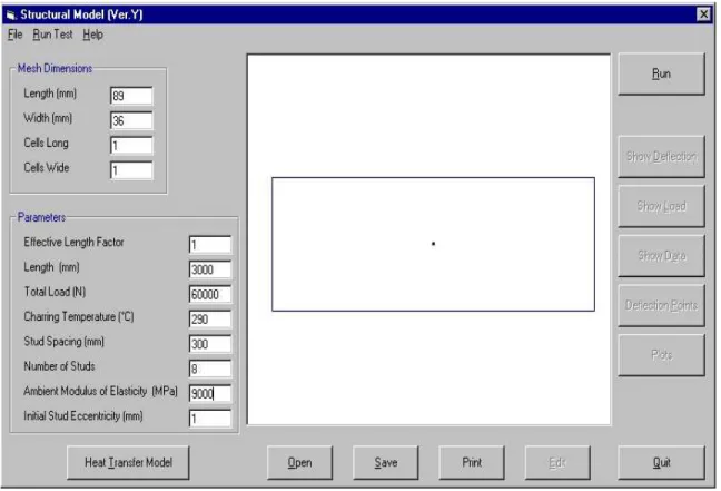
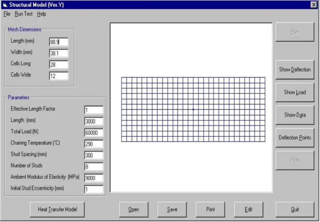
Figure 3.1 shows the first screen once the program is executed.
Figure 3.1. Main Screen (Default)
The user has several options to choose from before the Structural Response Model is executed. These are:
Option Description
• Heat Transfer Model
Allows the user to load the Wall-2D Database or run the Heat Transfer Model to generate time-temperature data
• Open Allows the user to open input, output or time-temperature data files
• Save Allows the user to save input data
• Print Allows the user to print the main screen
• Edit Allows the user to edit the time-temperature data
3.1.1 Importing data files
The user has the option of using previously-saved data to run the test. The user can open previously-saved input information from the main interface, time-temperature information and data from running the Forintek heat transfer model.
To import saved information from a previously-run test:
1. Click the Open button in the File menu (Figure 3.2), or click the Open button in the Main Window (Figure 3.3).
Figure 3.2. File Menu, Open
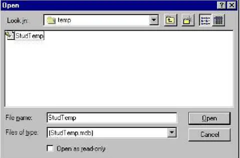
Figure 3.3. Open Button 2. Find and choose the saved file (Figure 3.4).
3. Click Load.
The Load command allows the user to open input files (.inp), time-temperature data files (.ttd), and output files (.out).
* When loading these data files, it is important that the mesh information is not changed. The data loaded corresponds to specific elements, and if those elements are changed / missing, the program will display an error. Other information, such as the applied load or charring temperature may be changed.
3.1.2 Heat transfer model (time-temperature database)
This option allows the user to import a database from the Wall 2D program into the Structural Response Model for analysis.
1. Select the Heat Transfer Model item in the File menu (Figure 3.5), or click the Heat Transfer Model button in the Main Window (Figure 3.6).
Figure 3.5. File Menu, Heat Transfer Model
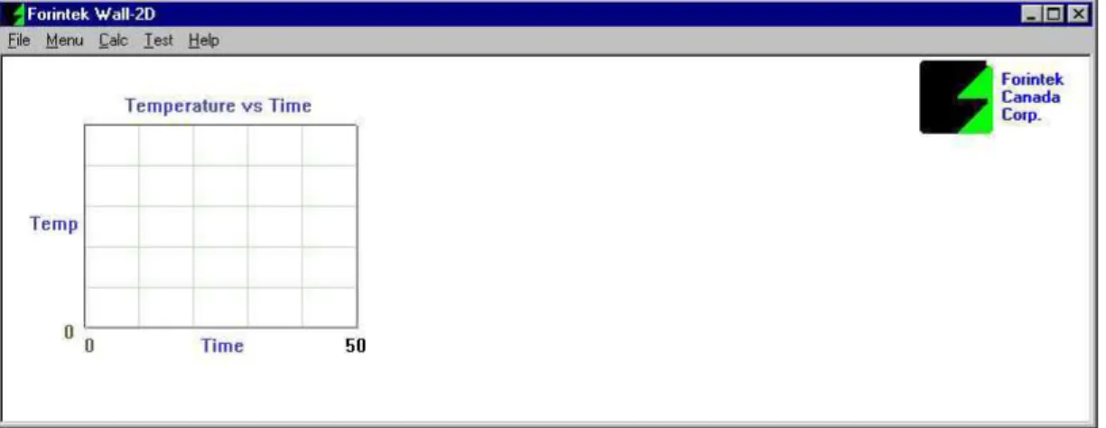
2. The window (Figure 3.7) will appear. The Run Wall-2D option will load the heat transfer program (Figure 3.8), and the Load Forintek Database option will allow the user to import saved time-temperature data from a previous run of the heat transfer model (Figure 3.9).
Figure 3.7. Heat Transfer Model / Forintek Database
Figure 3.8. Forintek Wall 2D
Figure 3.9. Load Forintek Database
3. When a Database file has been selected and loaded, the top pull down menu in (Figure 3.10) will allow you to select which table in the database to view.
4. Click on Exit (Figure 3.10) to return to the Main Screen (Figure 3.11).
Figure 3.11. Main Screen with Database Loaded
3.1.3 Editing time-temperature data
By selecting Edit from the File menu (Figure 3.12), or by clicking on the Edit button (Figure 3.13) the user can edit the time-temperature data.
Figure 3.12. File Menu, Edit
The Edit button will become active when either:
1. A time-temperature data file (.ttd) has been loaded;
2. Time-temperature data from the heat transfer model has been loaded; or 3. A user has manually entered time-temperature data.
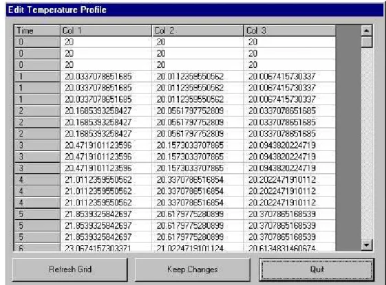
The Edit Temperature Profile window will be loaded. (Figure 3.14)
Figure 3.14. Edit Temperature Profile
1. Enter the corresponding temperatures into the grid. You may type them in directly, or cut and paste them from a spreadsheet or word processor.
2. When finished, click Keep Changes. 3. Click Quit.
The changes made by the user will appear highlighted in yellow. Should the user want to abort the changes, there are two options:
1. Click the Refresh Grid button, or
3.1.4 Saving input data
All of the user inputted information (parameters, mesh dimensions, etc.) may be saved and used in another run of the program. To save the input data:
1. Enter all the data in the main window.
2. Open the File menu, and select the Save button (Figure 3.15) or press the Save button in the Main Screen (Figure 3.16).
Figure 3.15. File Menu, Save
Figure 3.16. Save Button
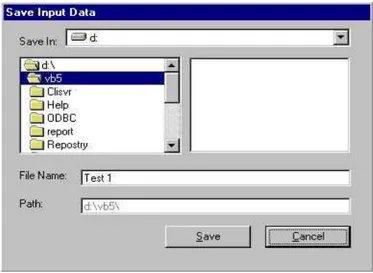
3. Select the directory where you would like this information to be saved by double-clicking it (Figure 3.17), type the file name and click Save. The file is saved with an “.inp” extension.
3.1.5 Printing the main screen
When printing, the user has the option of printing the entire window by selecting either the Print command from the File menu (Figure 3.18) or by clicking the Print button (Figure 3.19).
Figure 3.18. File Menu, Print
Figure 3.19. Print Button
3.1.6 Quitting the Structural Response Model
Selecting on Quit in the File menu (Figure 3.20) or clicking the Quit button (Figure 3.21) will exit the Structural Response Model.
Figure 3.20. File Menu, Quit
3.2 Execution
With all the information entered/loaded, the Structural Response Model is now ready to be executed. The user has the choice of running the Structural Response Model using either one input, or with multiple input files and one time-temperature database.
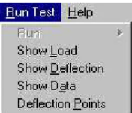
To choose between selecting one or multiple inputs, go to the Run Test menu (Figure 3.22).
Figure 3.22. Run Test Menu, Run 3.2.1 Single input
1. Select Run and then Single Input (Figure 3.23) or click the Run button. (Figure 3.24)
Figure 3.23. Run Test Menu, Run Single Input
Figure 3.24. Run Button
2. If there is insufficient data for the Structural Response Model to run, the user will be prompted (Figure 3.25) to either generate temperatures or to load a temperature file.
3. Clicking Yes will bring up the Input Time Steps window (Figure 3.26) which allows the user to determine the number of time steps. Clicking No will load the Load file menu (Figure 3.4) described earlier.
Figure 3.26. Input Time Steps
4. Clicking OK in Figure 2.26 will load the Edit Temperature Profile window (Figure 3.14), with only one column.
5. If there is sufficient data, the program will be executed and the Main Screen (Figure 3.27) will be displayed.
3.2.2 Multiple inputs
1. For multiple input files, select Run and then Multiple Inputs (Figure 3.28)
Figure 3.28. Run Test Menu, Run Multiple Inputs
2. The user will now be prompted (automatically) to select and load a Forintek heat transfer model database (Figure 3.9).
3. After selecting the desired database, the user must now select and load a batch file (Figure 3.29) containing the names of the desired input files.
Figure 3.29. Load Batch File
* The input files must be located in the same directory (folder) as the batch file. 4. The program will automatically run all the input files with the Forintek heat transfer
model database. The Plots window (see Figure 3.50) will be saved for each run, and a summary file will be generated.
5. The name of the Plots window is the name of the batch file followed by the name of the input file (for Figure 3.29, it would be “testInput1.bmp”, if the first input file was named “Input1.inp”).
6. The name of the summary file is the name of the batch file followed by Summary.txt (for Figure 3.29, it would be “test Summary.txt”).
3.3 Viewing the Results
Once the data has been inputted, the temperatures have been generated/loaded and the test has been run, there will be a choice of options. These are:
Option Description
• Show Deflection Displays a graph of deflection vs. time, and provides a table of values
• Show Load Displays a graph of maximum load vs. time, and provides a table of values
• Show Data Allows the user to view basic data, element data, or charring data
• Deflection Points Allows the user to view the deflection of the stud over time
• Plots Allows the user to view all of the plots simultaneously
The user can access these from the buttons on the right side of the main window (see Figure 3.27), as well as from the Run Test menu (Figure 3.30).
3.3.1 Show deflection
The Show Deflection window (Figure 3.31) is subdivided into two smaller windows: one contains the graph of deflection versus time, and the other window contains the plotted data.
Figure 3.31. Show Deflection
In the graph window, the graph is displayed along with the time at which the L/d or L/30 limit is exceeded and the corresponding maximum deflection.
The user has the choice of saving either the picture or the data, as well as printing the form or closing the window.
• To save the output data: 1. Click the Save Data button.
2. Select the directory where you would like this information to be saved by double-clicking it. (Figure 3.32)
Figure 3.32. Save Data 3. Enter a name for the file.
4. Click the Save button (the data is saved as (tab delimited) ASCII files).
• To save the graph, follow the same procedure for saving the data, except click the Save Picture button (this is saved as a .bmp format file).
• To print the entire form, click on the Print Form button.
3.3.2 Show load
The Show Load window (Figure 3.33) is subdivided into two smaller windows: one contains the graph of load versus time, and the other window contains the data that was plotted.
Figure 3.33. Show Load
In the graph window, the graph is displayed along with the time at which the structure fails and the corresponding applied load.
The buttons available in this window are identical in function and operation to those described in (3.3.1 above).
3.3.3 Show data
The Show Data window (Figure 3.34) is subdivided into two smaller windows: one contains the data, and the other window contains a visual representation of the wood stud. There are three buttons to display information, in addition to the Save Picture button, the Save Text button, and the Cancel button.
Figure 3.34. Show Data (Main)
The buttons available in this window are identical in function and operation to those described in (3.3.1 above), except that in (Figure 3.34), Save Data is replaced by Save Text, and Close is replaced by Cancel. There is no Print button for this form.
The File Menu (Figure 3.35) allows the user to save (Figure 3.36) either the picture or the text, or to cancel (Figure 3.37) and exit this window.
Figure 3.35. Data Window, File Menu
Figure 3.36. File Menu, Save
The Options Menu (Figure 3.38) allows the user to display either the basic data (Figure 3.39), the element data (Figure 3.40), or the charring data (Figure 3.41).
Figure 3.38. Data Window, Options Menu
Figure 3.39. Options Menu, Show Basic Data
Figure 3.40. Options Menu, Show Element Data
3.3.3.1 Show basic data
This button (Figure 3.42) displays general information, such as the number of columns, the number of rows, the number of time steps, the length and width of the stud. The charring times, element areas, the distance to the elemental centroids, as well as the element width and length are also displayed. In addition, the temperature at set time intervals is displayed for each element.
3.3.3.2 Show element data
This button displays particular information for a given element. In the graphical window, a picture of the wood stud will appear (Figure 3.43). The user must click on the desired element, and the data corresponding to that element will be displayed in the text window.
In addition, the coordinates of the element centroid will be displayed above the picture of the wood stud, once an element has been selected (Figure 3.44). The data displayed consists of the element number, the temperature and modulus of elasticity of the element (E) at one minute time intervals.
3.3.3.3 Show charring
This button allows the user to see how the wood stud is charred over the duration of the test. When the Show Charring button is clicked (Figure 3.45), the horizontal scroll bar will become active, and the user can then use the arrows to scroll from the beginning to the end of the test, and observe which elements char and when.
It is important to note that by holding down the slider in the scroll bar and dragging the mouse left or right, the user will not see what happens at all the time intervals; only the charring at the time the mouse button is released will be seen. (Figure 3.46)
3.3.4 Deflection points
This button displays a graph of how the deflection of the stud varies with respect to both height and time. There is also a data window on the right, which allows the user to view the deflection in time increments of five minutes, and at each minute the deflection data is given for every 100 mm of height (Figure 3.47).
Figure 3.47. Deflection Points
The user can also call up the data for a specific time by using the arrow in the uppermost text box. By clicking on the down arrow in this box, a list of time intervals will be displayed (Figure 3.48).
Once the desired time has been selected, click on the graph area. A green curve will be displayed, which is the deflection at the desired time. In addition, the particular information for the specific time can be viewed by scrolling down to the end of the data window. (Figure 3.49)
Figure 3.49. Deflection Points
The buttons available in this window are identical in function and operation to those described in (3.3.1 above).
3.3.5 Plots
This button allows the user to view all of the plots the program is capable of generating at the same time (Figure 3.50). These plots can then be printed or saved to a file.
Figure 3.50. Plots
* For the plot button to work, the user will have to have first opened the Show Deflection, Show Load and Deflection Points windows.
Figure 3.51. Plots, File Menu
The Plots form can be saved as (.bmp) from the File menu by clicking on Save Picture (Figure 3.51).
The entire form may be printed from the File menu by clicking on Print Form (Figure 3.51).
4.0 DOCUMENTATION
4.1 Online Help
An online help file is provided for reference. To access the help file: 1. Open the Help menu and choose Index. (Figure 4.1).
Figure 4.1. Help Menu, Index
2. Enter the first few letters of the word being searched for in the text box or scroll down the list of topics (Figure 4.2).
Figure 4.2. Index (eg. studs)
3. View the help text by ensuring the right topic is highlighted, and click the Display button.
If the words See Also (Figure 4.2) in the upper right-hand corner of the screen become highlighted and underlined, click them to view a list of related topics (Figure 4.3).
Figure 4.3. Related Topics (eg. studs)
4.2 User Manual
This manual is also available as part of the program, and can be accessed by opening the Help menu and selecting User Manual (Figure 4.4).
Figure 4.4. Help Menu, User Manual
4.3 About / Version Information
By clicking on the Help menu and selecting About, version information can be obtained regarding this program (Figure 4.5).
5.0 REFERENCES
1. Takeda, H.; Kouchleva, S. Heat Transfer Model WALL2D, Version 2.0, Forintek Canada, Forintek Canada Corp., 1999.
2. Bénichou, N.; Morgan, D.; Hum, J. Structural Response Model of Wood Stud Wall Assemblies Technical Manual, Research Report 130, IRC, NRC, Ottawa, Ontario, March 2003.
3. Bénichou, N.; Morgan, D.; Hum, J. Structural Response Model of Wood Stud Wall Assemblies Theory Manual, Research Report 128, IRC, NRC, Ottawa, Ontario, March 2003.