Costs of Climate Mitigation Policies
Y.-H. Henry Chen, Mustafa Babiker, Sergey Paltsev, John Reilly
Report No. 292
March 2016
The MIT Joint Program on the Science and Policy of Global Change combines cutting-edge scientific research with independent policy analysis to provide a solid foundation for the public and private decisions needed to mitigate and adapt to unavoidable global environmental changes. Being data-driven, the Program uses extensive Earth system and economic data and models to produce quantitative analysis and predictions of the risks of climate change and the challenges of limiting human influence on the environment—essential knowledge for the international dialogue toward a global response to climate change.
To this end, the Program brings together an interdisciplinary group from two established MIT research centers: the Center for Global Change Science (CGCS) and the Center for Energy and Environmental Policy Research (CEEPR). These two centers—along with collaborators from the Marine Biology Laboratory (MBL) at Woods Hole and short- and long-term visitors—provide the united vision needed to solve global challenges.
At the heart of much of the Program’s work lies MIT’s Integrated Global System Model. Through this integrated model, the Program seeks to: discover new interactions among natural and human climate system components; objectively assess uncertainty in economic and climate projections; critically and quantitatively analyze environmental management and policy proposals; understand complex connections among the many forces that will shape our future; and improve methods to model, monitor and verify greenhouse gas emissions and climatic impacts. This reprint is one of a series intended to communicate research results and improve public understanding of global environment and energy challenges, thereby contributing to informed debate about climate change and the economic and social implications of policy alternatives.
Ronald G. Prinn and John M. Reilly,
Program Co-Directors
For more information, contact the Program office:
MIT Joint Program on the Science and Policy of Global Change Postal Address:
Massachusetts Institute of Technology 77 Massachusetts Avenue, E19-411 Cambridge, MA 02139 (USA) Location:
Building E19, Room 411 400 Main Street, Cambridge Access:
Tel: (617) 253-7492 Fax: (617) 253-9845
Email: [email protected]
1
Costs of Climate Mitigation Policies
Y.-H. Henry Chen, Mustafa Babiker, Sergey Paltsev, John Reilly Abstract
The wide range of cost estimates for stabilizing climate is puzzling to policy makers as well as researchers. Assumptions about technology costs have been studied extensively as one reason for these differences. Here, we focus on how policy timing and the modeling of economy-wide interactions affect costs. We examine these issues by restructuring a general equilibrium model of the global economy, removing elements of the model one by one. We find that delaying the start of a global policy by 20 years triples the needed starting carbon price and increases the macroeconomic cost by nearly 30%. We further find that including realistic details of the economy (e.g. sectoral and electricity technology detail; tax and trade distortions; capital vintaging) more than double net present discounted costs over the century. Inter-model comparisons of stabilization costs find a similar range, but it is not possible to isolate the structural causes behind cost differences. Broader comparisons of stabilization costs face the additional issue that studies of different vintages assume different policy starting dates, often dates that are no longer realistic given the pace of climate change negotiations. This study can aid in interpretation of estimates and give policymakers and researchers an idea of how to adjust costs upwards as the start of policy is delayed. It also illustrates that models that greatly simplify the realities of modern economies likely underestimate costs.
Contents
1. INTRODUCTION ... 1
2. ALTERNATIVE MODEL STRUCTURES AND POLICY TIMING ... 3
2.1 Regional and Sectoral Structure ... 3
2.2 Capital Vintaging ... 5
2.3 Domestic and International Trade Distortions ... 6
2.4 Structure of the Electricity Sector ... 8
2.5 Policy Timing and Discount Rates ... 9
3. SIMULATION DESIGN AND RESULTS ... 10
3.1 Simulation Design ... 10
3.2 The Effect of Policy Timing on Stabilization Costs ... 11
3.3 Results with Alternative Model Structures ... 12
3.4 Results with Various Discount Rates ... 14
4. CONCLUSION ... 16
5. REFERENCES ... 17
1 1. INTRODUCTION
Climate change is a serious concern that poses major risks, both for economic well-being and for the natural ecosystems on which we depend (IPCC, 2014). There is little question that the efforts to reduce emissions should be strengthened, but at what cost? The Stern Review (Stern, 2007) reasoned that the cost of stabilization at 500–550 ppm of carbon dioxide equivalent (CO2-eq) was annually about 1% of Gross World Product (GWP) looking out to the year 2050,
and damages of unabated climate change would require as much as a present-value 20% reduction (on average) in consumption per person worldwide. Comparing those benefits to mitigation costs made a strong case for rapid cuts in greenhouse gas emissions, with little reason to even consider further mitigation costs.
The Working Group III contribution to the Fifth Assessment Report (AR5) of the
Intergovernmental Panel on Climate Change (IPCC) focused on 450 ppm CO2–eq stabilization
(studies reported in this category achieved stabilization in a range of 430–480 ppm) and found considerably higher mitigation costs in terms of percentage loss in macroeconomic consumption (IPCC, 2014). Quoting from the summary for policymakers:
Scenarios in which all countries of the world begin mitigation immediately, there is a single global carbon tax, and all key technologies are available, have been used as a cost-effective benchmark for estimating macroeconomic mitigation costs. Under these assumptions, mitigation scenarios that reach atmospheric concentrations of about 450 ppm CO2-eq by 2100 entail losses in global consumption— not including benefits of
reduced climate change as well as co-benefits and adverse side-effects of mitigation—of 1% to 4% (median: 1.7%) in 2030, 2% to 6% (median: 3.4%) in 2050, and 3% to 11% (median: 4.8%) in 2100 relative to consumption in baseline scenarios that grows anywhere from 300% to more than 900% over the century.
The technical summary of the IPCC provides cost estimates of stabilization in the range of 480–530 ppm, more similar to Stern’s range (Edenhofer et al., 2014). The 25–75% likelihood cost range for that stabilization level is actually somewhat greater than the 430–480 ppm CO2
range at about 1.5–3.9% in 2050. The full range was from about 0.5% to over 5%. The top end of the even looser target of 530–580 ppm stabilization was even higher, at 11%. The varying ranges of cost estimates reflect variation in the sample of models simulating each stabilization level. For example, the 530–580 ppm range included results from 46 scenarios from 18 models (that came from 11 modeling groups), whereas the 430–480 ppm range included results from only 14 scenarios from 9 models (that came from 6 modeling groups). Given the broader sample, the full range for the 530–580 ppm is probably more representative of the range of disagreement in the modeling literature on stabilization costs.
The IPCC summary statement identifies some assumptions that suggest real costs could be higher than estimated: they assume a uniform global carbon tax—a very efficient mechanism for reducing emissions; they assume all technologies are available, but in reality alternatives like nuclear or carbon capture and storage may face public resistance, limiting availability and raising
2
costs; and they assume all nations participate, with mitigation policies beginning immediately— but this is certainly not the case especially since, given the publication date of the studies, “immediately” meant 2010 or 2015. With delay, sharper cuts are needed, which again would likely increase costs.
On the other hand, despite GHG mitigation costs, the IPCC reports that world economic activity grows 3 to 9 times over the century. The costs do not cause a 100-year decline in the economy, but instead shave less than a tenth or two from the GDP growth rate: instead of growing at 2.5% per year (which would increase economic activity by 9 times over 90 years) the growth rate might fall to 2.3 or 2.4% per year (even at the higher end of cost estimates), or if the base growth was 2% per year (increasing activity 6 times) then, with mitigation costs, it might fall to 1.8 or 1.9%.
Nevertheless, the costs at the high end are approaching Stern’s damage estimates, which are based on an equal weighting of future and present generations. Given that many of the greater damages estimated in the Stern Review are occurring far in the future, the net present value percentage consumption loss would be considerably lower for all categories of damages with a higher discount rate. The implication would be a more gradual emissions reduction. On the other hand, while the IPCC clearly suggests the Stern Review’s cost number was too low, the range in the IPCC’s cost estimate is enormous, making it important to try to resolve this wide range.
Obvious places to look for why the cost range is so large are assumptions about the cost of the low-carbon alternative energy sources. That aspect of the problem has been extensively explored in global scenarios by the IPCC (Edenhoffer et al., 2014) and in depth for the US in an Energy Modeling Forum exercise summarized in Clarke et al. (2015), as well as in many individual modeling studies. If costs of alternatives are more expensive or key alternatives are disallowed, macroeconomic costs will be higher. As shown in in Clarke et al. (2007), models with relatively low future costs delayed abatement with lower near-term costs compared with models that were less optimistic about the relative cost of non-fossil and fossil alternatives. While technological progress can reduce costs, in some cases early cost estimates may have been overly optimistic. For instance, in 2007 constant US dollars, the US Energy Information Administration’s (EIA’s) estimated overnight capital cost of advanced coal with CCS increased from around $3700/KW in 2010 (EIA, 2010) to nearly $6300/KW in 2015 (EIA, 2015).
In short, much work has explored the effect of technology cost and policy design. Less work has explored the effects of the timing of global policy, so the literature often compares results that assumed an optimal abatement trajectory from 2010–2015 to more recent studies, which include a later start date. Also underexplored is the structure of macro-energy-economic models. A recent exception, Gillingham et al. (2015) conducts a multi-model comparison, assessing uncertainty in economic and population growth and climate sensitivity on multiple output variables from a suite of integrated assessment models. While the study reveals differences and similarities in results, it is not able to isolate how individual structural assumptions in the models affect model results. We take a complementary approach with a single macro-energy-economic model, and progressively simplify the structure by removing realistic details of the economy that are often not represented in simpler energy-economic models. Our energy-economic model is among the more complex
3
models used in integrated assessment. It generates costs on the high end of the IPCC range. We conduct two sets of exercises. In the first, we explore the implications of delayed policy adoption; in the second, we gradually reduce the complexity of the model structure and analyze how that affects mitigation costs. The rest of the paper is organized as follows: Section 2 presents the alternative model structures and policy timing considered in this study, Section 3 discusses simulation design and analyzes results, and Section 4 provides conclusions.
2. ALTERNATIVE MODEL STRUCTURES AND POLICY TIMING
We use a recently updated version of the Economic Projection and Policy Analysis (EPPA) model (Chen et al., 2015). It is a computable general equilibrium (CGE) model of the world economy. CGE modeling has been widely used in various economy-wide analyses such as trade liberalization, the interaction between foreign direct investment and trade, optimal taxation, modeling of the roles of power sector technologies, and energy and environmental policies (Rutherford et al., 1997; Zhou and Latorre, 2014; Bovenberg and Goulder, 1996;
Tapia-Ahumada et al., 2015; van der Mensbrugghe, 2010).
A key element of this class of economic model is a full input-output (I/O) structure of the economy: goods produced by one sector may be used in other production sectors as intermediate goods, used by consumers and governments as final goods, or used as investment goods or exports. Factor inputs and factor markets are explicitly resolved. Multi-regional models include trade among regions in goods and services. The macro-economy of EPPA follows these same lines, with some unique features. It includes advanced energy conversion technologies and accounts for both greenhouse gases and conventional pollutants. In addition to labor and produced capital, the model resolves a number of natural resource factors including energy resources and land. The version of EPPA used here updates the main economic data of the model to the Global Trade Analysis Project Version 8 (GTAP 8) database with a benchmark year of 2007 (Narayanan et al., 2012). Costs of advanced technologies, pollution inventories, and emissions coefficients for carbon and other GHGs are also updated as described in Chen et al. (2015). Previous versions of the model are described in Babiker et al. (2001), Paltsev et al. (2005), and Reilly et al. (2012). We focus here on those elements of the model that we simplify.
2.1 Regional and Sectoral Structure
The model covers all countries of the world in 18 regions. Large economies (United States, Canada, Mexico, Japan, China, Russia, South Korea, Indonesia, India, Brazil) are each
represented as separate regions, and smaller economies are aggregated together to form geographically contiguous regions such as the European Union, the Middle East, or Africa, as shown in Table 1. The regional structure plays a role in our simulations through the inclusion or exclusion of tariffs and trade distortions.
The model includes 18 sectors (see Table 2), with the largest in economic terms for many countries being the Other Industries sector. Details in the Agriculture, Energy-Intensive
Industries, and Transportation sectors are included given the resource focus of the modeling even though for most regions they are a small share of output in terms of value added.
4 Table 1. Regions and abbreviations.
Abbr. Region Abbr. Region Abbr. Region
USA United States ROE Eastern Europe & Central Asia IND India
CAN Canada RUS Russia BRA Brazil
MEX Mexico REA East Asia AFR Africa
JPN Japan KOR South Korea MES Middle East
ANZ Australia, New Zealand & Oceania IDZ Indonesia LAM Latin America
EUR European Union+a CHN China ASI Rest of Asia
a
The European Union (EU-28) plus Norway, Switzerland, Iceland, and Liechtenstein.
Table 2. Sectors and abbreviations.
Abbr. Sector Abbr. Sector Abbr. Sector
CROP Agriculture - Cropsa ROIL Refined Oil ELEC: hydro Hydro Electricity
LIVE Agriculture - Livestocka GAS Gas EINT Energy-Intensive Industriesa
FORS Agriculture - Forestrya ELEC: coal Coal Electricity OTHR Other Industriesa
FOOD Food Productsa ELEC: gas Gas Electricity DWE Dwellingsa
COAL Coal ELEC: petro Petroleum Electricity SERV Servicesa
OIL Crude Oil ELEC: nucl Nuclear Electricity TRAN Commercial Transporta a Sectors aggregated together to form a single sector in scenarios showing the effect of aggregation on costs.
Table 3. Advanced technologies in the energy sector.
First generation biofuels Advanced gas Second generation biofuels Advanced gas w/ CCS
Oil shale Wind
Synthetic gas from coal Bio-electricity
Hydrogen Wind power combined with bio-electricity Advanced nuclear Wind power combined with gas-fired power Advanced coal w/ CCS Solar generation
We note that with less sectoral resolution, there is implicit substitution among intermediate inputs, and we hypothesize that sectoral aggregation would reduce costs by making implicit substitution away from energy intensive products like iron and steel, paper, chemicals, and cement production easier. To test this hypothesis, we restructure our basic model by combining the Agriculture sectors, Food Products, Energy-Intensive, Other, Dwellings, Services and Commercial Transport into a single sector with a single industry output. This eliminates all non-energy intermediate inputs, and therefore all output goes to final demand (households, government, investment, or exports).
In addition to sectors presented in Table 2, the energy sector is augmented with the inclusion of 14 advanced technologies that provide substitutes for conventional (existing) power
generation, natural gas, petroleum or liquid fuels refined from petroleum (Table 3). These advanced technologies remain separately identified in all simulations.
In our standard specification, coal, gas, and petroleum based electricity generation are imperfect substitutes. We simplify this by restructuring different generation types as producing
5
electricity outputs that are perfect substitutes. We maintain constraints on hydro generation expansion based on assessment of additional resources that can be developed in each region. We assume that existing nuclear capacity and sites can be maintained and relicensed at their current marginal production cost, but that any further nuclear expansion in a region must come from advanced nuclear, subject to a different cost structure.
2.2 Capital Vintaging
In our standard model we include capital vintaging, which captures two important
inflexibilities: (1) once investment occurs, capital must remain in the sector (or technology) in which it was placed until it depreciates; and (2) once built, the ability to substitute among inputs is limited. The first inflexibility is often termed irreversibility, and means that once the
investment is made, future decisions on whether to use it are based only on variable costs. This makes it more difficult for advanced technology to capture market share, as the price of output from the old technology can drop below full replacement cost—at least until the sunk capital depreciates away. The second inflexibility means that if relative prices change or the technology improves, the vintaged stock is unable to adjust to these new prices or update to the
characteristics of the new technology (e.g. higher-efficiency coal power generation). This gives less ability to substitute away from a fossil-based input. In our representation, only a portion of capital in any sector is vintaged, reflecting that some aspects of a plant’s physical structure or siting can be reused, and that plants may be retrofitted to take some advantage of substitution possibilities.
To represent vintaging in the model, capital is divided into two portions: 𝐾𝑀#, in which all new investment is malleable, and a vintaged, non-malleable portion 𝑉%,#, where n represents a particular vintage category and t represents the time period. Capital is region specific, and vintaged capital is sector specific. For simplicity, in the notation we suppress region and sector subscripts. For a given time period, 𝑛 = 1 is 5-year-old vintaged capital in a sector and region; 𝑛 = 2 and 𝑛 = 3 are the 10- and 15-year-old vintaged capital, respectively; and 𝑛 = 4 is capital older than 20 years. The dynamics of the malleable capital are described by:
𝐾𝑀# = 𝐼𝑁𝑉#/0+ 1 − 𝜃 1 − 𝛿 5𝐾𝑀
#/0 (1)
In Equation (1), 𝜃 is the fraction of the malleable capital that becomes non-malleable at the end of period 𝑡 − 1. 𝐼𝑁𝑉#/0 and 𝛿 are the investment and annual depreciation rate, respectively. The factor of 5 is used because the model is solved in five-year intervals. The newly formed non-malleable capital 𝑉0,# is the fraction, 𝜃, of the surviving malleable capital from the previous period:
𝑉0,# = 𝜃 1 − 𝛿 5𝐾𝑀#/0 (2)
With this structure capital has a lifetime of 25 years, but much capital—especially in the power sector and capital intensive industry—survives well beyond 25 years. To accommodate this, we slowly depreciate vintage 4 capital, updating its production coefficients in t + 1 to reflect the average of undepreciated vintage 4 stock at time t, with the newly added in t + 1 vintage 4
6
stock. We assume that the physical productivity of installed vintage capital does not depreciate until it reaches the final vintage. This reflects an assumption that, once in place, a physical plant can continue to produce the same level of output without further investment. This is in
conjunction with the assumption that (1 − 𝜃) of capital remains malleable and depreciates continuously. Heuristically, this can be seen as investment in a new physical plant to be part vintaged and part malleable, with the regular updates and replacement (short of the long-term replacement of a plant) accounted in the depreciation of malleable capital. This process can be described by:
𝑉9,#:0= 𝑉0,#; 𝑉=,#:9 = 𝑉9,#:0; 𝑉>,#:= = 𝑉=,#:9+ 1 − 𝛿 5𝑉
>,#:9 (3)
An implication of this formulation is that old capital can become obsolete if relative prices change. Big changes in relative prices—for example, if a high carbon tax is suddenly put in place—can push the rental price on old capital to zero, implying that it may cease operation, or only operate below full capacity. This reflects realities we see in the electric power sector where old, inefficient power plants are often idled except during peak demand periods, or if there are requirements or incentives to add renewable capacity when there is little or no demand growth. Morris et al. (2014) demonstrate this feature under example simulations.
Most models looking decades into the future, on the other hand, often assume capital is fully malleable without considering vintaging. If the time periods are 10 or 15 years, a policy is gradually implemented, and agents have perfect foresight that may not be a bad assumption. However, given tight stabilization goals where rapid reduction in emissions is required, this assumption means that a coal power plant in period 𝑡 can implicitly become a wind turbine in period 𝑡 + 1. In reality, with sunk costs, the coal-fired power plant may continue operating for years or decades despite carbon pricing. Advanced technologies must only beat the lower marginal variable costs, not the full cost of the replacing the coal power plant. The sunk cost in old technology means a higher carbon tax will be required for advanced technologies to build early. Put another way, a coal plant prematurely retired will result in lost investment (or stranded assets). While vintaging of capital is a standard feature of our model, to examine the
implications, we will also consider a putty-putty setting with no capital vintaging. 2.3 Domestic and International Trade Distortions
In an idealized economy without externalities, economic welfare is optimized when prices reflect the marginal cost of producing goods. Taxes imposed to simply raise revenue distort the level of economic activities (production, consumption, trade flows, etc.), as opposed to those specifically formulated to correct for externalities. Bovenberg and Goulder (1996) pointed out that existing tax distortions may exacerbate the welfare loss of an abatement policy. Taking a production activity as an example, the distortionary effect of a tax can be shown as a mixed complementarity problem (MCP). With no tax distortion, the problem is:
7
In Problem (4), 𝑀𝐶 and 𝑃 are marginal cost and price, which is the marginal revenue of producing 𝑄, respectively. When the output 𝑄 is positive, the marginal cost should equal the marginal revenue. When taxes are introduced, the problem becomes:
1 + 𝑡𝑖 ∙ 𝑀𝐶 − 1 − 𝑡𝑜 ∙ 𝑃 ≥ 0; 𝑄 ≥ 0 ; 1 + 𝑡𝑖 ∙ 𝑀𝐶 − 1 − 𝑡𝑜 ∙ 𝑃 ∙ 𝑄 = 0 (5) In Problem (5), one can think of the tax rates, 𝑡𝑖 and 𝑡𝑜, as those levied on the supplier and user of the good, respectively. With a positive 𝑡𝑖, producing 𝑄 becomes more expensive. Similarly, a positive 𝑡𝑜 makes the output less attractive to the user. In either case, less output 𝑄 is produced. The same logic applies to a subsidy, which is nothing more than a negative tax. One can derive an effective tax rate, 𝑡𝑖G, that combines both 𝑡𝑜 and 𝑡𝑖 by dividing the first inequality in Problem (5) by 1 − 𝑡𝑜:
𝑡𝑖G = #H:#I
0/#I (6)
This simply recognizes that the user price 𝑃 (to which 𝑡𝑜 is applied) includes 𝑀𝐶 ∙ (1 + 𝑡𝑖). For most goods and services, the primary tax is an excise (sales or value added) tax—here interpretable as a user tax. In the case of inputs such as labor or capital, both the user and the supplier may pay a tax. In the US, suppliers of labor pay tax on earned income and toward the payroll tax, while employers also pay part of the payroll tax. Similarly, investors (suppliers of capital) pay taxes on capital earnings and companies pay a tax on profits. International trade distortions enter as tariffs or subsidies on exports (supplier tax) or tariffs on imports (user tax).
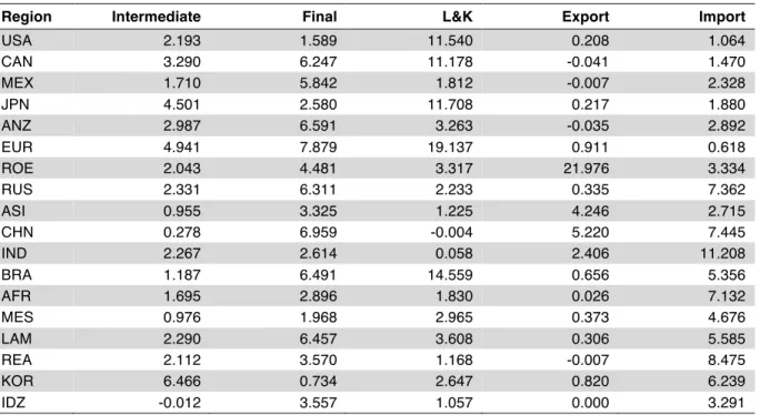
The GTAP data provides sector-specific taxes for all goods, inputs, imports and exports, and these are applied in our standard formulation aggregated to the regions and sectors of the model. The detailed tax rates are given in the Appendix. For illustrative purposes, Table 4 shows average tax rates aggregated to intermediate and final goods, labor, capital, exports and imports. All taxes are in terms of a supplier tax, as in Equation (6). The average tax rates presented in the table are calculated using the base-year value share of each commodity or input.
While we are able to use sector-specific rates for all goods and inputs, each is represented as an average tax rate for that input or good in that sector. In the case of a flat excise tax, this is appropriate. For more complex tax structures (e.g. progressive income taxes), the distortionary effect of the tax on an individual depends on the marginal tax rate that person or entity faces. Given that the GTAP database only provides average tax rates, we are likely underestimating the distortionary interaction effect of carbon pricing and taxes for countries with progressive tax rates. Aggregation across countries or sectors would also tend to reduce the distortionary effect. Capturing the effect of marginal tax rates requires more structure on household income than we have in EPPA. For an example that incorporates US marginal tax rates see Rausch et al. (2011).
To examine the implications of these tax distortions and possible interactions with mitigation policy, we consider alternative model structures that (1) eliminate all domestic tax distortions and (2) eliminate all international trade distortions.
8 Table 4. Average percentage tax rates in EPPA.
Region Intermediate Final L&K Export Import
USA 2.193 1.589 11.540 0.208 1.064 CAN 3.290 6.247 11.178 -0.041 1.470 MEX 1.710 5.842 1.812 -0.007 2.328 JPN 4.501 2.580 11.708 0.217 1.880 ANZ 2.987 6.591 3.263 -0.035 2.892 EUR 4.941 7.879 19.137 0.911 0.618 ROE 2.043 4.481 3.317 21.976 3.334 RUS 2.331 6.311 2.233 0.335 7.362 ASI 0.955 3.325 1.225 4.246 2.715 CHN 0.278 6.959 -0.004 5.220 7.445 IND 2.267 2.614 0.058 2.406 11.208 BRA 1.187 6.491 14.559 0.656 5.356 AFR 1.695 2.896 1.830 0.026 7.132 MES 0.976 1.968 2.965 0.373 4.676 LAM 2.290 6.457 3.608 0.306 5.585 REA 2.112 3.570 1.168 -0.007 8.475 KOR 6.466 0.734 2.647 0.820 6.239 IDZ -0.012 3.557 1.057 0.000 3.291
2.4 Structure of the Electricity Sector
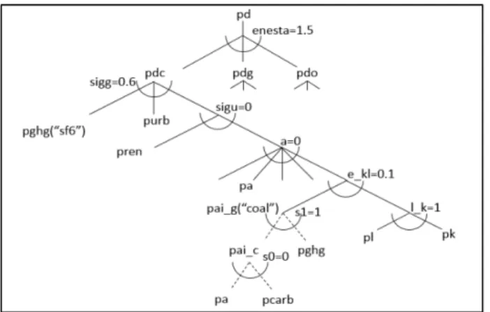
We use Constant Elasticity of Substitution (CES) production functions (and the special cases of Leontief and Cobb-Douglas functions) throughout our standard model formulation. We overcome the restriction that all pairs of inputs have identical elasticities of substitution by creating a nest structure. Figure 1 illustrates the nest structure for fossil-based electricity generation. Each nest can have an elasticity of substitution that applies to input pairs within that nest. As discussed above, these elasticities apply to production from malleable capital. Once vintaged, elasticities of substitution are zero. The production technology in the model is represented by a cost function based on the duality theorem. Taking the fossil-based power sector aggregation as an example, the index for the marginal cost of the aggregated output, denoted by 𝐶, can be expressed as:
𝐶 = 𝛼K 𝑝𝑑𝑐/𝑝𝑑𝑐 0/P+ 𝛼Q 𝑝𝑑𝑔/𝑝𝑑𝑔 0/P+ 𝛼I 𝑝𝑑𝑜/𝑝𝑑𝑜 0/P 0/(0/P) (7)
where 𝛼K, 𝛼Q, and 𝛼I are the value shares for coal-fired, gas-fired, and oil-fired generation technologies, and 𝑝𝑑𝑐, 𝑝𝑑𝑔, and 𝑝𝑑𝑜 are price indices for coal-fired, gas-fired, and oil-fired generation options, respectively. The bar over each price index denotes the benchmark value. 𝜎 is the elasticity of substitution on the top nest, which is denoted by 𝑒𝑛𝑒𝑠𝑡𝑎 in Figure 1. Vintaged production for each generation technology has a different sub-nest. The output from vintage production is homogenous to that from malleable production of that generation type, which means both outputs have the same price index. While Equation (7) is for the top nest CES, other sub-nests are formulated in the same fashion.
9
Figure 1. Production structure for fossil-based generation.1
The structure of Equation (7) means that electricity from oil, gas, or coal are imperfect substitutes for one another. While electricity from any generation type is indistinguishable, the intuition for imperfect substitution is that different generation forms play different roles in supplying base, shoulder and peak loads. The lower fuel cost and higher capital costs of coal generation, and penalties associated with ramping it, make it a more likely option for base load generation. Gas generation can have lower capital costs and a higher fuel cost, and it can be ramped more quickly; therefore, it is often preferred for providing peak capacity or adding flexibility for periods that require rapid ramping. The imperfect substitution can also indirectly capture differences in prices of fuels within a region. Within our model formulation there is a single price for refined oil, gas, or coal used in electricity in each region. In reality, generation located near a coal mine mouth or natural gas field may face much lower prices than in the rest of the region. To the extent that the mix of generation types in the base data reflect these
intra-regional differences, one might expect stickiness in substitution as relative prices change. The share-preserving nature of the CES production allows some—but not complete—substitution toward the generation type whose relative cost drops. Econometric studies find generally low substitution elasticities among fuels in electric generation, supporting this characterization.
While there is a logic for and evidence of imperfect substitution among generation types, over the long term with bigger relative prices changes this approach may unduly constrain the ability to substitute among generation types. Thus, we restructure the model so that the three fossil generation types are perfect substitutes.
2.5 Policy Timing and Discount Rates
Many of the results in the literature assume that a global climate policy would begin in the next year or two from the start of the research. Often by the time the research is published and
1 𝑝𝑑 is the price index for aggregated fossil-based generation; 𝑝𝑑𝑐, 𝑝𝑑𝑔, and 𝑝𝑑𝑜 are price indices for coal-fired,
gas-fired, and oil-fired generation; 𝑝𝑐𝑎𝑟𝑏, 𝑝𝑔ℎ𝑔, 𝑝𝑢𝑟𝑏, and 𝑝𝑟𝑒𝑛 are price indices for CO2 emissions, non-CO2
GHGs, urban pollutants, and the price index for paying the renewable credit, respectively; 𝑝𝑎, 𝑝𝑎𝑖_𝑐, and 𝑝𝑎𝑓_𝑔 are price indices for various Armington goods; 𝑝𝑙 and 𝑝𝑘 are prices of labor and capital. The elasticity on the top of each nest is presented with both the notation and value.
10
finds its way into a review, the start date of the policy is already history. We start an “optimal” global path to stabilization in years ranging from 2010 to 2030, which allows for at least an heuristic update of older studies. This update is necessary given that near-term policy appears to have been set in place through 2025 or 2030 (based on the outcome of recent international negotiations—see Jacoby and Chen, 2015; Reilly et al., 2015); additionally, given those policies, likely emissions pathways remain well above two-degree stabilization. The optimal stabilization path we consider is represented by imposing a uniform global carbon tax that rises at a specified discount rate over time. When the policy is delayed, a higher starting carbon tax will be needed to meet a given carbon budget. Lowering the discount rate (while keeping other things equal) will also necessitate a higher initial carbon tax, as it requires more near-term reduction. While in most exercises we use a discount rate of 4%, we also present results under different reduction paths based on various discount rates.
Finally, another subtle difference in comparison among studies is the discount rate. In
forward-looking general equilibrium models, the discount rate is endogenous and depends on the pure rate of time preference and the growth rate of the economy. In our recursive-dynamic formulation, we apply an exogenous discount rate. As applied it has two effects. First, since we simulate a price path that rises at the discount rate, the price path and timing of emissions reductions are affected. A higher discount rate means a lower initial carbon price and less early abatement, with a more steeply rising rate and more abatement in later periods. Second, the net present value cost calculation is directly affected by the choice of discount rate.
3. SIMULATION DESIGN AND RESULTS 3.1 Simulation Design
We simulate a stabilization scenario under different policy scenarios and model structures. The first year of the model run is 2007, which is the base year of GTAP 8 (Narayanan et al., 2012), the main economic database of our model. Starting from 2010, the model solves in 5-year intervals. The projected global GDP of our model in 2100 under the reference scenario is around 7.5 times higher than the 2010 level, while the corresponding cumulative emissions from 2010 to 2100 is about 5100 GtCO2. Because international negotiations focus on a 2°C warming target,
we develop policy scenarios consistent with meeting that target. We follow Sokolov et al. (2015) and target a cumulative carbon budget of 900 GtC (3300 GtCO2) emitted from 1870 through
2100. This carbon budget is consistent with CO2 concentrations of 480–530 ppm by the end of
the 21st century, corresponding to a 50% chance of meeting a 2°C target (IPCC, 2014). As in the IPCC (2014), we impose a uniform carbon tax across regions to ensure the budget is met. Other non-CO2 GHGs are priced similarly based on their global warming potential (GWP) levels.
We consider two sets of exercises: (1) exploring policy timing by shifting the start of the policy from 2010 to 2030 in 5-year increments; and (2) stripping away, one-by-one, complexities in our economic model to see how those changes affect estimated macroeconomic costs.
11
3.2 The Effect of Policy Timing on Stabilization Costs
Scenarios with varying timing of the start of the stabilization scenario are listed in Table 5. These simulations are conducted with the standard model formulation. By assumption the carbon tax rises at an annual rate of 4%, simulating optimal timing of reductions for an assumed
discount rate of 4%. To achieve the aforementioned carbon budget, the required initial CO2 tax
(in constant 2010 US dollars) is $47/tCO2 if the policy could have started in 2010, and it more
than triples to $154/tCO2 if the policy implementation is delayed to 2030 (Figure 2).
The imposition of the significant carbon tax results in an immediate sharp reduction in emissions in the year in which it is implemented (Figure 3). For instance, the initial reduction is 7.9 Gt, 9.2 Gt, 12.8 Gt, 16.8 Gt, and 21.8 Gt for a policy start date of 2010, 2015, 2020, 2025, and 2030, respectively.
Although countries have agreed to policies and measures designed to reduce emissions from a business-as-usual projection, evaluation of these proposed policies suggest that global emissions would continue to rise through 2030 to 37 GtCO2 by one estimate (Reilly et al., 2015). While
somewhat below the 46.5 Gt in 2030 in the reference scenario, it is far above the roughly 23 GtCO2 that would be consistent with an optimal carbon tax.
Table 5. Scenarios varying the policy start date.
Policy Scenario Policy Start Annual Discount Rate
S2010_D4 2010 4%
S2015_D4 2015 4%
S2020_D4 2020 4%
S2025_D4 2025 4%
S2030_D4 2030 4%
Figure 2. Initial carbon taxes for scenarios with various policy timings.
47 60 80 108 154 0 20 40 60 80 100 120 140 160 180 S2010_D4 S2015_D4 S2020_D4 S2025_D4 S2030_D4 $/ tC O2
12
Figure 3. Global CO2 emissions with various policy timings.
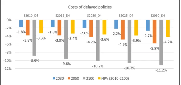
Figure 4. Costs of policies in 2030, 2050, 2100 with various policy timings. NPV shows the net present value of the cost over 2010–2100.
The economic cost results reveal that delaying the abatement policy would substantially increase the mitigation costs (Figure 4). For instance, if the policy were postponed to 2030, compared to the scenario where the policy starts from 2010, the mitigation costs in 2050 and 2100 would rise by 52.0% and 26.4%, respectively, and the present value of the cost for the time period 2010–2100 would increase by nearly 29%, from a 3.3% loss of consumption to 4.4%.
3.3 Results with Alternative Model Structures
Table 6 presents model structure variants developed for the second exercise. For these
scenarios we begin with the optimal policy starting in 2020. We replace price targets by emission caps for each model period and each region equal to the level of emissions achieved in the BASE
0 10 20 30 40 50 60 70 80 Gt C O2 Global CO2 Reference S2010_D4 S2015_D4 S2020_D4 S2025_D4 S2030_D4 -‐1.8% -‐1.8% -‐2.0% -‐2.2% -‐2.7% -‐3.8% -‐3.9% -‐4.2% -‐4.9% -‐5.8% -‐8.9% -‐9.6% -‐10.2% -‐10.7% -‐11.2% -‐3.3% -‐3.4% -‐3.6% -‐3.9% -‐4.2% -‐12% -‐10% -‐8% -‐6% -‐4% -‐2% 0% S2010_D4 S2015_D4 S2020_D4 S2025_D4 S2030_D4
Costs of delayed policies
13
scenario in each period, where a starting CO2 price equal to $80 per ton was required to meet the
cumulative emissions target. This ensures that the same level of emissions is achieved in all cases. Given the structural changes across scenarios, we expect that a fixed carbon tax would give a different (and likely greater) level of abatement as we strip away complexities.
The alternative model structures yield somewhat different business-as-usual emissions (Figure 5). Removing the vintaging structure slightly decreases the emission levels because older capital is less energy efficient than newer capital. Eliminating tax distortions, on the other hand, increases economic output and emissions. Sectoral aggregation does not substantially change the emissions profile. Stripping off the CES structure for conventional fossil generation facilitates the switch from coal to gas, whose driving factors include the cost for coal-fired power considered in the model (Chen et al., 2015). The easier coal-to-gas switch explains why global emissions under this setting are the lowest up to the middle of the century. Removal of the CES structure then results in higher emissions for later years. This is because without the CES structure, the flexibility to switch to the least-cost generation source is increased. This leads to more gas generation, lower electricity prices, and eventually substantial increase in electricity use and generation. Thus, in later years, even with less coal and more gas use, CO2 emissions are
ultimately higher without the CES structure. Table 6. Alternative model structures.
Scenario Structural Setting
BASE Base parameterization of EPPA6
NV BASE + vintaging removed
NVD NV + domestic tax distortion removed NVT NVD + all other tax distortions removed
AGG-NVT NVT + an aggregated non-fossil and non-electricity sector AGGE-NVT AGG-NVT + perfect substitution among fossil generation options
Figure 5. Global reference CO2 emissions with various model settings.
0 20 40 60 80 Gt C O2 Global CO2 Base NV NVD NVT AGG-‐NVT AGGE-‐NVT
14
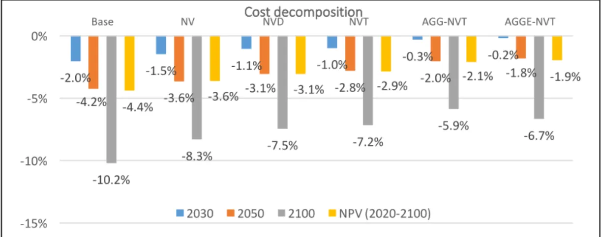
When the emissions reduction policy is imposed, regardless of model complexities, emissions are invariant by design under the considered emission cap, yielding the same emissions as those under the price target scenario S2020_D4 (Table 5). The results with alternative model structural settings show that taking out the vintaging structure reduces net present value costs by 18% (from 4.4 to 3.6%), with the biggest reductions earlier in the century (Figure 6). Removing domestic tax distortions lower the costs by another 14% (from 3.6 to 3.1%), and removing international tax distortions reduces the NPV cost by another 7% (from 3.1 to 2.9%). Again, the cost reductions are greatest earlier in the century. Sectoral aggregation eliminates the interdependency between the disaggregated sectors, and thus makes it easier to cut emissions, reducing the net present value cost by another 28% (from 2.9 to 2.1%). Removing the CES structure used in conventional fossil generations further reduces the NPV cost by 10% (from 2.1 to 1.9%). However, while nearer-term costs are lower in this case, longer-term costs are higher. This higher cost can be traced to the higher projected business-as-usual emissions in later years (Figure 5).
Altogether, incorporating economic realities such as limited generation substitution in
electricity, sectoral disaggregation, domestic and international distortions and capital asset fixity more than doubles the estimated macroeconomic cost of the stabilization policy we implement here, increasing net present value costs over the period through 2100 from 1.9% to 4.4%.
3.4 Results with Various Discount Rates
As previously noted, different discount rate assumptions can also lead to different costs and time paths of emissions. In this final set of simulations, we again generate optimal stabilization price paths for discount rates of 2, 3, 4, and 5%—a range that reflect different views on the underlying risk free market return on investment. This range includes the IPCC’s standard 5% discount rate assumption (Table SPM2 in IPCC, 2014). Since the IPCC generally uses much more simplified macroeconomic models, to compare our results we simulate these scenarios with the most simplified model structure that we developed in the preceding section (AGGE-NVT). Starting the policy in 2020, under each discount rate regime, we “re-optimize” the carbon price path for AGGE-NVT by finding a new uniform initial price with the goal of meeting a carbon budget consistent with the 480–530 ppm target. As hypothesized, the higher the initial discount rate, the lower the initial carbon price (Figure 8). At a discount rate of 5% a price of $52/tCO2 is
required, and at 2% this rises to $184/tCO2.
In terms of the net present value cost of the policies, the AGGE-NVT structure using a 5% discount rate generates an identical 2.2% NPV cost of the policy that we estimate for the IPCC. While the NPV costs are identical, the IPCC time paths vary from our estimate (Figure 7). The median mitigation costs (in terms of the aggregated consumption) the IPCC reported are −1.7%, −2.7%, and −4.7% for 2030, 2050, 2100, with the corresponding ranges for the 16th to 84th
percentile being [−0.60%, −2.14%], [−1.48%, −4.17%] and [−2.44%, −10.55%],
respectively (IPCC, 2014). For this case, our estimates for 2030, 2050, and 2100 are 0.8, 2.1, and 9.7%, respectively—lower than the IPCC estimates for early years and rising above their median estimate in the second half of the century.
15
Figure 6. Costs of policies in 2030, 2050 and 2100 with various model settings. NPV shows the net present value of the cost over 2010–2100.
Figure 7. Initial carbon taxes for scenarios with various discount rates.
Figure 8. Costs of policies in 2030, 2050, and 2100 with various discount rates. NPV shows the net present value of the cost over 2010–2100, discounted in each scenario at the same rate assumed for the price path. The IPCC AR5 did not report NPV costs for the century. We interpolated from the reported results to estimate an NPV value for the IPPC summary costs. Additionally, while the IPCC used a 5% discount rate in some calculations, the modeling groups summarized in Table SPM2 (IPCC, 2014) likely used a range of discount rates.
-‐2.0% -‐1.5% -‐1.1% -‐1.0% -‐0.3% -‐0.2% -‐4.2% -‐3.6% -‐3.1% -‐2.8% -‐2.0% -‐1.8% -‐10.2% -‐8.3% -‐7.5% -‐7.2% -‐5.9% -‐6.7% -‐4.4% -‐3.6% -‐3.1% -‐2.9% -‐2.1% -‐1.9% -‐15% -‐10% -‐5%
0% Base NV NVD NVT AGG-‐NVT AGGE-‐NVT
Cost decomposition 2030 2050 2100 NPV (2020-‐2100) 52 77 118 184 0 50 100 150 200 RS2015_D5 RS2015_D4 RS2015_D3 RS2015_D2 $/ tC O2
Initial carbon taxes for scnearios with various discount rates
-‐2.0% -‐1.4% -‐1.1% -‐0.8% -‐1.7% -‐2.5% -‐2.3% -‐2.2% -‐2.1% -‐2.7% -‐4.8% -‐6.1% -‐7.7% -‐9.7% -‐4.7% -‐3.2% -‐2.9% -‐2.6% -‐2.2% -‐2.2% -‐12% -‐10% -‐8% -‐6% -‐4% -‐2% 0% RS2015_D2 RS2015_D3 RS2015_D4 RS2015_D5 IPCC AR5 Consumption loss under agge-‐nvt
16 4. CONCLUSION
The wide range of cost estimates for stabilizing climate is puzzling to policy makers as well as researchers. Assumptions about technology costs and the efficiency of the policy instrument used to reduce emissions are obvious candidates for explaining cost differences, and these have been explored extensively in the literature. The starting time of a global policy and discount rate for the optimal path of abatement may also affect costs. Different models make different
assumptions about the discount rate, and studies done years ago (or those which optimistically assume the immediate adoption of a strong global policy) may generate a wider range of costs. This contributes to a puzzling range of results in the literature.
An additional source of cost differences is the complexity (or realism) of the simulated economy in which energy investment and other greenhouse gas abatement decisions are made. The economics literature strongly indicates that capital vintaging (i.e. irreversibilities in investment decisions), interaction with domestic and international tax distortions, the complex interdependency among sectors of the economy, and complexities within the electricity sector would likely reduce the flexibility of agents responding to a carbon price, and hence increase costs of abatement. Global models able to simulate global policies that meet IPCC review criteria generally do not include these complexities. This study illustrates that models that lack the complexities of a real economy likely underestimate mitigation costs.
When we simulate a model structured to eliminate complexities of the economic system using a timing and discount rate similar to those assumed in the IPCC, we find that our net present value cost of achieving a 2°C target is identical to the median estimate of the IPCC (at 2.2%). Notably, this is more than twice the cost estimated in the Stern Review. This may reflect, in part, that the Stern Review is now 10 years old, and studies reviewed at that time likely assumed the global policy would start in 2010 or earlier. By our estimate, if we could have started a global policy in 2010, the cost would be 8% less than if started in 2020 compared to our base policy runs. Unfortunately, while international negotiations have made progress in getting commitments from countries to abate, those commitments are insufficient to drive emissions down, which we find an optimal policy would do immediately upon implementation. Hence, if we are able to eventually get on an optimal path of emissions abatement toward the 2°C target, it will likely not be until 2030 or later, further increasing the costs. Our estimate is that delaying the start to 2030 would increase the cost by another 14%.
Finally, we find that including more realistic complexities of world economies with our
standard model formulation explains why our costs are more than twice the median estimate of the IPCC. The economic cost of unabated climate change has proven very difficult to estimate, but the risks are significant. Warming of several degrees would eventually lead to meters of sea level rise and inundate many coastal cities. This effect of unabated global warming alone seems enough to justify the costs of stabilizing greenhouse gas emissions—even with higher estimated costs. These higher cost estimates do not justify a less-stringent abatement policy; instead, they highlight the need to design the most efficient policies possible—with special concern for the costs imposed both on lower-income economies and low-income households in economies everywhere.
17 Acknowledgments
We gratefully acknowledge the financial support for this work provided by the MIT Joint Program on the Science and Policy of Global Change through a consortium of industrial and foundation sponsors and Federal awards, including the U.S. Department of Energy, Office of Science under DE-FG02-94ER61937 and the U.S. Environmental Protection Agency under XA-83600001-1. For a complete list of sponsors and the U.S. government funding sources, please visit http://globalchange.mit.edu/sponsors/all. We are thankful for insights and edits from Professor Henry D. Jacoby and Jamie Bartholomay in refining the study. All remaining errors are our own.
5. REFERENCES
Babiker, M.B., J.M. Reilly, M. Mayer, R.S. Eckaus, I. Sue Wing and R.C. Hyman, 2001: The MIT Emissions Prediction and Policy Analysis (EPPA) Model: Revisions, Sensitivities, and Comparisons of Results. MIT Joint Program on the Science and Policy of Global Change Report 71, Cambridge, MA (http://globalchange.mit.edu/files/document/MITJPSPGC_Rpt71.pdf).
Bovenberg, A. Lans and Lawrence H. Goulder, 1996: "Optimal Environmental Taxation in the Presence of Other Taxes: General Equilibrium Analyses." American Economic Review 86(4): 985–1000. Chen, Y.-H.H., S. Paltsev, J.M. Reilly, J.F. Morris and M.H. Babiker, 2015: The MIT EPPA6 Model:
Economic Growth, Energy Use, and Food Consumption. MIT Joint Program on the Science and Policy of Global Change Report 278, Cambridge, MA
(http://globalchange.mit.edu/files/document/MITJPSPGC_Rpt278.pdf).
Clarke, L.E., A.A. Fawcett, J.P. Weyant, J. McFarland, V. Chaturvedi and Y. Zhou, 2015: Technology and U.S. emissions reductions goals: Results of the EMF 24 modeling exercise. The Energy Journal 35(Special Issue 1): 9–32.
Edenhofer O., R. Pichs-Madruga, Y. Sokona, S. Kadner, J.C. Minx, S. Brunner, S. Agrawala, G. Baiocchi, I.A. Bashmakov, G. Blanco, J. Broome, T. Bruckner, M. Bustamante, L. Clarke, M. Conte Grand, F. Creutzig, X. Cruz-Núñez, S. Dhakal, N.K. Dubash, P. Eickemeier, E. Farahani, M. Fischedick, M. Fleurbaey, R. Gerlagh, L. Gómez-Echeverri, S. Gupta, J. Harnisch, K. Jiang, F. Jotzo, S. Kartha, S. Klasen, C. Kolstad, V. Krey, H. Kunreuther, O. Lucon, O. Masera,
Y. Mulugetta, R.B. Norgaard, A. Patt, N.H. Ravindranath, K. Riahi, J. Roy, A. Sagar, R. Schaeffer, S. Schlömer, K.C. Seto, K. Seyboth, R. Sims, P. Smith, E. Somanathan, R. Stavins, C. von Stechow, T. Sterner, T. Sugiyama, S. Suh, D. Ürge-Vorsatz, K. Urama, A. Venables, D.G. Victor, E. Weber, D. Zhou, J. Zou, and T. Zwickel, 2014: Technical summary. In: Climate Change 2014: Mitigation of
Climate Change. Contribution of Working Group III to the Fifth Assessment Report of the Intergovernmental Panel on Climate Change [Edenhofer, O., R. Pichs-Madruga, Y. Sokona,
E. Farahani, S. Kadner, K. Seyboth, A. Adler, I. Baum, S. Brunner, P. Eickemeier, B. Kriemann, J. Savolainen, S. Schlömer, C. von Stechow, T. Zwickel and J. C. Minx (eds.)]. Cambridge University Press, Cambridge, United Kingdom and New York, NY, USA.
(http://report.mitigation2014.org/report/ipcc_wg3_ar5_technical-summary.pdf)
EIA [Energy Information Administration], 2010: Annual Energy Outlook, U.S. Energy Information Administration, Washington, DC.
EIA [Energy Information Administration], 2015: Annual Energy Outlook, U.S. Energy Information Administration, Washington, DC.
Gillingham, K., W.D. Nordhaus, D. Anthoff, G. Blanford, V. Bosetti, P. Christensen, H. McJeon, J. Reilly and Paul Sztorc, 2015: Modeling Uncertainty in Climate Change: A Multi-Model Comparison. National Bureau of Economic Research working paper w21637 (Oct. 2015) (http://www.nber.org/papers/w21637).
18
IPCC [Intergovernmental Panel on Climate Change], 2014: Summary for policymakers. In: Climate
Change 2014: Mitigation of Climate Change. Contribution of Working Group III to the Fifth Assessment Report of the Intergovernmental Panel on Climate Change [Edenhofer, O.,
R. Pichs-Madruga, Y. Sokona, E. Farahani, S. Kadner, K. Seyboth, A. Adler, I. Baum, S. Brunner, P. Eickemeier, B. Kriemann, J. Savolainen, S. Schlömer, C. von Stechow, T. Zwickel and J.C. Minx (eds.)]. Cambridge University Press, Cambridge, United Kingdom and New York, NY, USA. Jacoby, H.D. and Y.H.-H. Chen, 2015: Launching a New Climate Regime. MIT Joint Program on the
Science and Policy of Global Change Report 286, Cambridge, MA (http://globalchange.mit.edu/files/document/MITJPSPGC_Rpt286.pdf).
Morris, J., J. Reilly and Y.-H.H. Chen, 2014: Advanced Technologies in Energy-Economy Models for Climate Change Assessment. MIT Joint Program on the Science and Policy of Global Change Report
272, Cambridge, MA (http://globalchange.mit.edu/files/document/MITJPSPGC_Rpt272.pdf). Narayanan, G., Badri, T.W. Hertel and T.L. Walmsley, 2012: GTAP 8 Data Base Documentation –
Chapter 1: Introduction. Center for Global Trade Analysis, Department of Agricultural Economics, Purdue University, March (https://www.gtap.agecon.purdue.edu/resources/download/5673.pdf). Nordhaus, W.D., 2007. Review: A Review of the "Stern Review on the Economics of Climate Change”
Journal of Economic Literature 45(3): 686–702
Paltsev, S., J.M. Reilly, H.D. Jacoby, R.S. Eckaus, J. McFarland, M. Sarofim, M. Asadoorian and M. Babiker, 2005: The MIT Emissions Prediction and Policy Analysis (EPPA) Model: Version 4. MIT Joint Program on the Science and Policy of Global Change Report 125, Cambridge, MA (http://globalchange.mit.edu/files/document/MITJPSPGC_Rpt125.pdf).
Rausch, S., G.E. Metcalf and J.M. Reilly, 2011, Distributional impacts of carbon pricing: A general equilibrium approach with micro-data for households. Energy Economics 33(S1): S20–S33. Reilly, J., J. Melillo, Y. Cai, D. Kicklighter, A. Gurgel, S. Paltsev, T. Cronin, A. Sokolov and
A. Schlosser, 2012: Using Land to Mitigate Climate Change: Hitting the Target, Recognizing the Tradeoffs. Environmental Science and Technology 46(11), 5672–5679.
Reilly, J., S. Paltsev, E. Monier, H. Chen, A. Sokolov, J. Huang, Q. Ejaz, J. Scott, J. Morris and
C.A. Schlosser, 2015: Energy and Climate Outlook: Perspectives from 2015. MIT Joint Program on the Science and Policy of Global Change, Cambridge, MA (http://globalchange.mit.edu/Outlook2015). Roberts, D., 2015: Economists agree: economic models underestimate climate change. VOX Energy &
Environment. VOX Media. December 8, 2015. http://www.vox.com/2015/12/8/9869918/economists-climate-consensus
Rutherford, T.F., E.E. Rutström and D. Tarr, 1997: Morocco’s free trade agreement with the EU: a
quantitative assessment, with David Tarr and Elizabet Rutström. Economic Modelling 14(2): 237–269. Sokolov, A., S. Paltsev, H. Chen, M. Haigh, and R. Prinn, 2015: Climate Stabilization at 2°C and “Net
Zero” Emissions. Working paper. MIT Joint Program on the Science and Policy of Global Change. Stern, N., 2007. The Economics of Climate Change: The Stern Review. Cambridge and New York:
Cambridge University Press.
Tapia-Ahumada, K., C. Octaviano, S. Rausch, and I. Pérez-Arriaga, 2015: Modeling intermittent
renewable electricity technologies in general equilibrium models, Economic Modelling 51: 242–262. van der Mensbrugghe, D., 2010: The Environmental Impact and Sustainability Applied General Equilibrium
(ENVISAGE) Model. The World Bank. (http://siteresources.worldbank.org/INTPROSPECTS/ Resources/334934-1314986341738/Env7_1Jan10b.pdf)
Zhou, J. and M.C. Latorre, 2014: How FDI influences the triangular trade pattern among China, East Asia and the U.S.? A CGE analysis of the sector of Electronics in China, Economic Modelling
19 Appendix
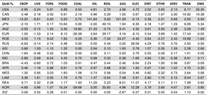
Table A1. The average tax rate of intermediate consumption by sector.
Unit:% CROP LIVE FORS FOOD COAL OIL ROIL GAS ELEC EINT OTHR SERV TRAN DWE
USA -2.95 -3.24 5.91 0.99 9.55 4.81 2.70 4.06 4.72 2.02 0.83 2.13 6.17 20.30 CAN 0.48 0.18 3.50 0.61 2.19 0.96 0.29 1.50 5.67 3.22 1.67 3.30 19.92 19.38 MEX -13.20 -6.61 0.00 0.20 0.72 141.84 0.02 101.59 -0.13 0.38 0.31 0.69 0.05 0.00 JPN -2.10 1.71 0.17 10.64 0.00 0.00 49.10 1.94 6.30 4.18 1.47 1.23 8.06 5.34 ANZ -3.93 -3.15 1.20 3.40 19.80 21.33 -0.74 9.41 4.32 3.61 3.93 2.38 3.39 1.49 EUR 1.00 -1.53 2.14 6.12 -26.39 2.84 29.17 4.16 8.15 5.54 3.69 1.42 17.44 -0.05 ROE 4.35 1.15 9.02 1.93 -3.25 0.36 -7.34 24.27 -4.40 3.84 -2.27 2.45 19.89 -1.84 RUS -6.63 -3.14 2.74 0.48 0.00 0.00 0.49 0.00 28.09 4.29 0.76 0.70 2.95 0.00 ASI 0.66 1.03 -1.15 1.32 0.00 2.94 0.10 1.65 3.76 1.07 0.30 1.59 2.28 2.66 CHN -1.84 -0.46 0.52 0.09 0.00 0.00 0.11 0.00 3.70 0.55 0.09 0.17 1.01 0.00 IND -5.89 2.69 6.54 4.20 0.75 0.68 0.33 0.38 -1.69 4.85 1.50 -0.38 9.91 0.11 BRA -4.43 -0.60 0.72 1.03 0.91 0.47 0.44 0.46 6.64 2.24 1.00 0.98 3.87 0.09 AFR 0.46 1.16 0.88 0.61 0.76 0.97 5.88 2.00 1.93 0.97 1.54 1.52 4.70 0.35 MES 1.30 0.95 3.03 1.83 1.06 0.74 0.58 0.04 3.46 0.82 0.32 0.73 3.64 0.06 LAM 3.38 1.61 2.05 1.70 0.79 1.47 -3.54 7.48 5.91 2.80 1.74 2.12 9.04 2.67 REA 0.71 0.32 2.28 1.17 1.93 11.29 0.22 8.01 11.57 4.17 0.11 2.11 7.08 0.62 KOR -4.69 0.66 1.57 15.24 -39.68 0.00 35.83 4.96 12.28 2.79 3.60 4.67 2.81 3.85 IDZ 0.09 0.55 0.26 0.01 0.00 0.00 0.00 -2.67 -5.57 0.01 0.05 0.04 1.13 0.00
* Each sector may have different input tax rates for various inputs. The average rate is calculated based on input value shares.
Table A2. Tax rates on final consumption by sector.
Unit:% CROP LIVE FORS FOOD COAL OIL ROIL GAS ELEC EINT OTHR SERV TRAN DWE
USA 5.34 3.15 2.91 9.76 5.88 0.00 26.24 2.32 3.15 6.05 7.78 0.53 0.00 0.00 CAN -1.61 -1.26 3.37 34.50 54.42 7.24 66.78 14.48 12.17 19.46 20.38 3.14 0.00 -0.16 MEX 0.13 0.08 0.00 9.12 0.00 0.00 28.30 38.12 12.65 13.75 25.37 2.16 0.00 0.00 JPN 4.89 4.76 4.97 4.98 0.00 0.00 68.57 23.71 8.25 4.94 4.89 2.21 4.99 0.00 ANZ 4.07 1.42 5.69 26.68 12.09 0.00 82.24 2.97 10.18 14.03 14.46 4.64 0.00 1.71 EUR -0.78 7.18 11.57 17.04 52.47 23.34 125.89 56.43 36.08 16.59 18.50 3.97 -0.08 4.32 ROE 0.81 1.11 0.76 7.94 27.07 47.31 118.20 23.57 16.34 1.85 4.53 1.14 0.54 -1.50 RUS 4.24 3.96 6.88 34.84 67.29 0.00 17.18 -16.00 2.21 25.82 13.79 -0.74 0.00 0.00 ASI 1.41 1.68 2.61 7.71 0.00 9.87 18.05 8.71 4.58 2.54 4.85 2.36 -1.01 2.89 CHN 0.41 0.21 4.58 12.27 17.82 0.00 12.18 -0.01 6.82 11.15 8.83 5.67 8.49 15.29 IND -3.13 0.10 0.35 3.55 2.20 0.00 79.09 -3.68 -11.31 9.54 4.70 0.54 -1.23 0.00 BRA 9.80 4.78 6.68 15.17 0.00 0.00 94.17 34.33 23.51 18.70 18.34 3.15 0.00 0.00 AFR 0.36 0.85 1.21 7.10 -0.01 0.82 27.86 -16.01 3.22 5.03 4.78 1.73 0.12 0.06 MES 0.13 1.20 3.50 2.80 1.13 0.19 8.45 8.01 2.12 1.73 2.53 1.60 3.08 0.44 LAM 5.09 2.63 2.85 13.40 22.79 19.00 58.16 22.47 22.03 10.49 14.66 3.00 0.00 0.10 REA 1.22 0.36 0.25 7.90 5.43 14.19 21.31 19.50 3.66 8.15 5.09 1.14 0.42 0.21 KOR 0.00 0.06 0.01 1.48 0.00 0.00 77.11 55.49 0.00 0.39 1.23 0.00 0.00 0.00 IDZ 1.36 1.19 3.42 8.23 0.00 0.00 4.54 -0.90 0.36 4.20 5.20 2.93 0.00 0.89
* The tax rate of final consumption is the average of private and public consumption calculated based on the value shares.
20 Table A3. Tax rates on labor income by sector.
Unit:% CROP LIVE FORS FOOD COAL OIL ROIL GAS ELEC EINT OTHR SERV TRAN DWE
USA 7.67 8.13 15.06 15.06 15.06 15.06 15.06 15.06 15.06 15.06 15.06 15.06 15.06 15.06 CAN -1.95 1.69 16.04 16.04 16.04 16.04 16.04 16.04 16.04 16.04 16.04 16.04 16.04 16.04 MEX 1.88 0.86 5.58 5.58 5.58 5.58 5.58 5.58 5.58 5.58 5.58 5.58 5.58 5.58 JPN 11.77 14.32 18.48 18.48 0.00 0.00 18.48 18.48 18.48 18.48 18.48 18.48 18.48 18.48 ANZ -0.21 0.76 3.44 3.41 4.17 4.02 3.66 3.79 3.78 3.74 3.93 3.87 3.87 4.45 EUR 19.21 15.67 35.97 35.96 38.36 24.65 32.10 30.97 37.50 37.96 37.39 36.23 35.07 28.82 ROE 3.22 7.22 5.74 5.66 14.99 7.15 12.15 9.79 15.80 6.62 6.21 5.01 7.10 9.48 RUS 2.27 2.27 2.27 2.27 2.27 2.27 2.27 2.27 2.27 2.27 2.27 2.27 2.27 0.00 ASI 1.17 0.95 1.38 1.33 1.45 1.39 1.71 1.44 1.39 1.70 1.60 1.62 1.49 1.57 CHN 0.00 0.01 0.00 0.05 0.00 0.00 0.00 1.94 0.03 0.03 0.06 0.21 0.25 0.00 IND 0.06 0.06 0.06 0.06 0.06 0.06 0.06 0.06 0.06 0.06 0.06 0.06 0.06 0.06 BRA 25.91 25.91 25.91 25.91 25.91 25.91 25.91 25.91 25.91 25.91 25.91 25.91 25.91 25.91 AFR 2.09 2.24 1.89 2.25 2.98 2.23 2.78 1.32 2.61 2.71 2.53 2.56 2.63 2.00 MES 7.85 6.28 6.72 5.61 8.46 2.22 3.61 6.83 10.91 7.31 6.12 7.09 6.65 13.56 LAM 5.23 5.07 4.50 5.11 0.91 5.25 5.93 8.81 4.33 5.30 4.98 5.94 5.77 8.22 REA 1.30 1.05 1.54 1.12 1.29 1.67 0.75 0.62 1.27 1.24 1.18 1.17 1.58 2.28 KOR -2.90 -1.08 4.96 4.96 4.96 0.00 4.96 4.96 4.96 4.96 4.96 4.96 4.96 4.96 IDZ 1.64 1.64 1.64 1.64 1.64 1.64 1.64 1.64 1.64 1.64 1.64 1.64 1.64 1.64
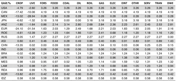
Table A4. Tax rates on capital income by sector.
Unit:% CROP LIVE FORS FOOD COAL OIL ROIL GAS ELEC EINT OTHR SERV TRAN DWE
USA -4.79 -2.60 3.26 3.26 3.26 3.26 3.26 3.26 3.26 3.26 3.26 3.26 3.26 3.26 CAN -17.42 -10.06 4.19 4.19 4.19 4.19 4.19 4.19 4.19 4.19 4.19 4.19 4.19 4.19 MEX -13.02 -28.94 0.28 0.28 0.28 0.28 0.28 0.28 0.28 0.28 0.28 0.28 0.28 0.28 JPN -6.62 -1.32 3.18 3.18 0.00 0.00 3.18 3.18 3.18 3.18 3.18 3.18 3.18 3.18 ANZ -1.85 -1.64 0.86 2.14 3.14 2.80 2.68 2.84 2.36 2.23 2.61 2.45 2.53 2.81 EUR -24.10 -31.54 1.63 2.03 1.29 2.49 1.68 2.21 2.03 1.83 1.93 2.05 1.91 2.16 ROE -4.61 -12.39 1.23 1.23 1.64 1.66 1.01 2.41 0.68 1.18 1.20 1.18 1.16 1.20 RUS -3.05 1.47 2.27 2.27 2.27 2.27 2.27 2.27 2.27 2.27 2.27 2.27 2.27 0.00 ASI 0.60 0.41 0.46 0.44 0.28 0.49 0.86 0.40 0.85 0.91 0.83 0.91 0.89 1.43 CHN -13.35 0.02 0.00 0.09 0.00 0.00 0.00 1.94 0.10 0.03 0.06 0.25 0.25 0.15 IND 0.06 0.06 0.06 0.06 0.06 0.06 0.06 0.06 0.06 0.06 0.06 0.06 0.06 0.06 BRA -0.02 -0.96 1.24 1.24 1.24 1.24 1.24 1.24 1.24 1.24 1.24 1.24 1.24 1.24 AFR 1.19 1.20 1.19 1.24 1.71 1.35 0.66 0.81 0.96 1.38 1.06 1.37 1.22 1.41 MES 0.98 1.03 0.95 0.97 0.52 1.05 1.23 1.14 1.00 1.59 1.52 1.31 1.23 1.32 LAM 1.24 0.98 1.01 0.85 0.64 0.85 1.29 1.18 0.68 0.85 1.05 1.23 1.24 0.94 REA 0.96 0.99 1.75 0.89 1.56 1.44 0.70 1.71 0.86 0.85 1.25 1.03 1.20 1.31 KOR -13.82 -8.01 0.42 0.42 0.42 0.00 0.42 0.42 0.42 0.42 0.42 0.42 0.42 0.42 IDZ 0.58 0.58 0.58 0.58 0.58 0.58 0.58 0.58 0.58 0.58 0.58 0.58 0.58 0.58
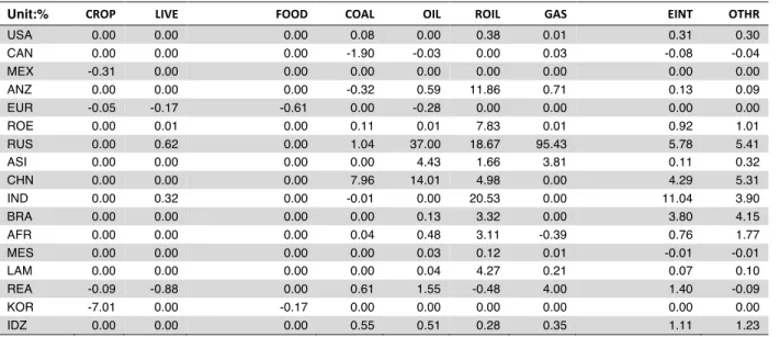
21 Table A5. The average export tax rates by sector.
Unit:% CROP LIVE FOOD COAL OIL ROIL GAS EINT OTHR
USA 0.00 0.00 0.00 0.08 0.00 0.38 0.01 0.31 0.30 CAN 0.00 0.00 0.00 -1.90 -0.03 0.00 0.03 -0.08 -0.04 MEX -0.31 0.00 0.00 0.00 0.00 0.00 0.00 0.00 0.00 ANZ 0.00 0.00 0.00 -0.32 0.59 11.86 0.71 0.13 0.09 EUR -0.05 -0.17 -0.61 0.00 -0.28 0.00 0.00 0.00 0.00 ROE 0.00 0.01 0.00 0.11 0.01 7.83 0.01 0.92 1.01 RUS 0.00 0.62 0.00 1.04 37.00 18.67 95.43 5.78 5.41 ASI 0.00 0.00 0.00 0.00 4.43 1.66 3.81 0.11 0.32 CHN 0.00 0.00 0.00 7.96 14.01 4.98 0.00 4.29 5.31 IND 0.00 0.32 0.00 -0.01 0.00 20.53 0.00 11.04 3.90 BRA 0.00 0.00 0.00 0.00 0.13 3.32 0.00 3.80 4.15 AFR 0.00 0.00 0.00 0.04 0.48 3.11 -0.39 0.76 1.77 MES 0.00 0.00 0.00 0.00 0.03 0.12 0.01 -0.01 -0.01 LAM 0.00 0.00 0.00 0.00 0.04 4.27 0.21 0.07 0.10 REA -0.09 -0.88 0.00 0.61 1.55 -0.48 4.00 1.40 -0.09 KOR -7.01 0.00 -0.17 0.00 0.00 0.00 0.00 0.00 0.00 IDZ 0.00 0.00 0.00 0.55 0.51 0.28 0.35 1.11 1.23
* An export tax rate may vary across export destinations. The average rate is calculated using the export value share of each destination region.
Table A6. Tax rates on imports by sector.
Unit:% CROP LIVE FORS FOOD COAL OIL ROIL GAS ELEC EINT OTHR
USA 2.18 0.23 0.19 3.08 0.00 0.00 0.68 0.00 0.00 0.98 1.57 CAN 0.22 7.41 0.02 16.84 0.00 0.00 0.32 0.03 0.00 0.47 1.29 MEX 5.52 0.60 1.19 3.18 0.01 0.00 0.78 0.00 0.03 1.57 3.10 JPN 12.60 4.31 0.11 19.62 0.00 0.00 0.35 0.00 0.00 0.72 1.30 ANZ 0.96 0.54 0.31 3.63 0.00 0.00 2.63 0.00 0.00 2.12 4.72 EUR 2.47 1.22 0.06 3.56 0.00 0.00 0.14 0.00 0.00 0.31 0.83 ROE 13.79 4.34 0.80 14.40 0.06 1.81 1.18 1.03 0.97 2.94 3.82 RUS 5.72 6.22 7.29 17.72 0.14 0.02 3.97 0.06 0.00 8.13 8.26 ASI 7.12 3.99 2.18 10.71 0.37 0.72 1.76 0.04 0.00 4.07 2.94 CHN 9.08 13.38 0.44 8.36 2.91 0.20 4.57 0.00 0.00 22.92 3.81 IND 45.48 12.78 6.33 78.28 31.40 9.94 13.83 9.43 0.00 14.93 10.42 BRA 1.97 2.77 3.20 6.15 0.00 0.00 0.19 0.00 0.00 6.75 9.97 AFR 10.65 8.99 6.65 17.17 2.46 1.24 6.81 0.00 0.16 7.21 8.66 MES 5.61 1.90 4.65 13.01 0.13 0.05 4.11 2.00 0.33 4.89 6.12 LAM 7.10 3.34 3.94 11.60 2.10 2.01 4.78 0.03 0.00 4.86 7.60 REA 7.56 4.24 3.79 14.55 5.23 4.03 11.49 0.00 0.70 6.65 11.51 KOR 208.92 11.76 0.22 30.41 0.00 2.99 4.40 2.28 0.00 3.36 3.84 IDZ 2.37 2.93 1.33 9.02 0.00 0.14 1.74 0.00 0.00 4.54 4.20
* An import tax rate may vary across origins. The average rate is calculated using the import value share of each origin region.