Cramér-Rao bounds for matched field tomography and ocean acoustic tomography

Cramer-Rao Bounds for Matched Field Tomography

and Ocean Acoustic Tomography

by

Peter M. Daly

B.S.E.E., University of Rhode Island (1993)

Submitted to the Department of Electrical Engineering and Computer Science

in partial fulfillment of the requirements for the degree of

Master of Science in Electrical Engineering and Computer Science

at the

MASSACHUSETTS INSTITUTE OF TECHNOLOGY

February 1997

_MvAR

_{0 6}

₁₉₉₇

@ Peter M. Daly, MCMXCVII. All rights reserved.

n

The author hereby grants to MIT permission to reproduce and distribute publicly

paper and electronic copies of this thesis document in whole or in part, and to grant

others the right to do so.

A uthor ...

...

... ...

Department of Electrical Engineering an Computer Science

January 15, 1997

Certified by ... ..

...

....

... .B.

Baggeroer

Arthur B.

Baggeroer

Ford Professor of Electrical and Ocean Engineering

Thesis Supervisor

Accepted by ... ... .•... .. , ...

Arthur C. Smith

Chairman, Departmental Committee on Graduate Students

I

Cram'r-Rao Bounds for Matched Field Tomography

and Ocean Acoustic Tomography

by

Peter M. Daly

Submitted to the Department of Electrical Engineering and Computer Science on January 15, 1997, in partial fulfillment of the

requirements for the degree of

Master of Science in Electrical Engineering and Computer Science

Abstract

This paper demonstrates a technique for solving the Cramer-Rao lower estimation bounds of environ-mental parameters applied to Matched Field Tomography (MFT) and Ocean Acoustic Tomography (OAT). MFT is a parameter estimation method which processes narrowband signals, using the inter-ference pattern generated between elements in a sonar array. OAT, another estimation technique, relies on acoustic travel times between a source and receiver; consequently, wideband signals are used to provide high time resolution. OAT exploits signal coherence over a selected bandwidth, while MFT does not. With knowledge of the Crambr-Rao bounds, one can determine the mini-mum variance attainable for an estimator of any environmental parameter, as well as determining the coupling between any set of parameters in the ocean environment. This information is useful for evaluating present estimation techniques, determining the feasibility and expected performance of new estimators, and finding how changes in one parameter can affect the estimation of other parameters in the ocean.

Attention was focused on modeling a range independent shallow water environment with a sediment layer and hard bottom. For a source and receiver spaced 15 km apart, four sound velocity profile parameters were estimated. A comparison was made between the relative performance of MFT and OAT. At low SNR levels, OAT has superior performance over MFT. Above certain SNR levels, similar performance was observed for both MFT and OAT. Under constant energy conditions, minimum standard deviations decrease as signal bandwidth increases. Coupling between parameters appears to be independent of SNR and inversion method (OAT vs. MFT), and only slightly influenced by signal bandwidth. Parameter selection is very important in determining the CRB; improper selection leads to artificially high estimation bounds.

This work was supported by the United States Navy, Office of Naval Research, under contracts N00014-93-1-0774 and N00014-90-J-1725.

Thesis Supervisor: Arthur B. Baggeroer

Acknowledgments

First of all, I would like to thank my parents for teaching me an excellent work ethic. I would like to thank Prof. Arthur B. Baggeroer for giving me this research topic, laying the foundation for the work described in this thesis, and donating his old 486 for use as an X-terminal on my desk. I would also like to thank Prof. Henrik Schmidt, who was always able to answer my quick questions, and pointed me toward SuperSNAP when KRAKEN failed.

I would like to thank the students and staff of MIT's Ocean Engineering Acoustics Group for all their help. Thanks to Pierre Elisseeff for showing me his KRAKEN modefile reading code. Thanks to Brian Sperry and Kathleen Wage for cleaning up PRUFER, and to Brian again for showing me how to calculate the Af for wideband acoustic propagation. I would like to thank Dr. Joe Bondaryk for his help with power spectral estimation, as well as his insights on parameter coupling and SNR calculation.

Thanks to the Office of Naval Research for sponsoring this work, through the NDSEG fellowship program (Contract N00014-93-1-0774), and the ATOC program (Contract N00014-90-J-1725).

Finally, and most importantly, thanks to those civilian engineers in the United States Navy who allowed me to rip their computers apart and load Linux on them, so I could run batch jobs at night. Without their array of computational power, this thesis would never have been completed in a timely manner. Thanks to Ken for approving this, and to Andy for supplying the first test machine. Thanks to both Jim and Diane for keeping me focused. Thanks to Brian for pointing me toward Bucker's implementation of Green's function.

Contents

1 Introduction 9

1.1 R oadm ap . . . . 10

1.2 Background Information . ... . . .... .... .... .... ... 10

1.2.1 Underwater Acoustic Propagation ... ... 10

1.2.2 Normal Mode Theory ... 12

1.2.3 Green's Function ... 15

1.2.4 Matched Field Processing ... 16

1.2.5 Ocean Acoustic Tomography ... 17

1.2.6 Matched Field Tomography ... 19

1.3 Previous W ork ... ... 21

1.3.1 CRB derivation ... ... ... 21

1.3.2 Applications of CRB to MFT and OAT ... .. 23

1.4 Sum m ary . .. .. .. ... . .. .. ... .. .. .. . ... ... .. 26

2 Theory and Formulation 27 2.1 Crambr-Rao Bound ... 28

2.2 Mechanics of the CRB ... 28

2.3 Application of the CRB to MFT and OAT ... ... 30

2.3.1 Matched Field Tomography ... 32

2.4 Ocean Acoustic Tomography ... 35

2.5 Sum m ary ... ... ... 41

3 Results 42 3.1 Environment .. . ... 42

3.1.1 Source and Receivers ... 3.1.2 Signal to Noise Ratio ...

3.1.3 Parameters ...

Minimum standard deviation . . . . Correlation Coefficients . . . . 3.3.1 High Parameter Correlation E 4 Conclusions

4.1 Summary ... 4.2 Contributions . ... 4.3 Future Work ... A Computational Procedure

A.1 Perturbation Magnitude ... A.1.1 Application to test case ...

A.2 Frequency Spacing ...

A.2.1 Calculating the optimal Af . A.3 Normal Mode, Green's Function, and

:nvironment

A.4 Simulation Hardware ...

. . . . . 44 CRB 68 . . . .. . . . .. . . . . 69 . . . .. . . . .. . . . . 72 . . . .. . . . .. . . . . 75 . . . .. . . .. . . . 75 . . . . . 78 calculation . .. . . . 79

List of Figures

1-1 Simplified acoustic environment. . ... ... 11

1-2 Simplified acoustic waveguide ... ... 12

1-3 Normal modeshapes and eigenvalues for a fictitious shallow water environment. . . . 15

1-4 Sample MFP ambiguity function[l]... . . . . ... . 18

1-5 Sample tomographic configuration ... 19

1-6 Tolstoy's MFT scenario, using air-dropped explosive charges. . . . . 20

1-7 Convergence zone scenario. ... 24

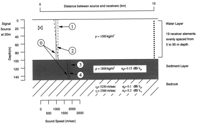
3-1 Pekeris shallow water environment. ... 42

3-2 Shallow water environment under study, with four environmental parameters shown. 43 3-3 Normalized source signal, with bandwidths of 10, 50, and 100 Hz . ... 45

3-4 CRB results for SNR of-20 dB ... 57

3-5 CRB results for SNR of-10 dB ... .... 58

3-6 CRB results for SNR of +20 dB. ... 59

3-7 Correlation coefficients for SNR of -20 dB. . ... ... 60

3-8 Changes to environment for high parameter correlation. . ... 61

3-9 CRB results for SNR of +10 dB, uncorrelated parameters. . ... 62

3-10 CRB results for SNR of +10 dB, correlated parameters. . ... 63

A-1 Flowchart of computational process ... 69

A-2 Variability of Green's Function ... .... 70

A-3 Variability of Green's Function ... 71

A-4 Linearity test for Green's Function ... ... 72

A-5 Plot of perturbations for parameter 1: water column sound speed, evaluated at 200 H z. . . . . 73

A-6 Plot of perturbations for parameter 1: water column sound speed, evaluated at 200 Hz. 74 A-7 Plot of group velocities for modified Pekeris profile. . ... 76 A-8 Plot of minimum and maximum group slowness 1/u, for modified Pekeris profile... 77 A-9 Plot of difference between minimum and maximum group slowness 1/un for modified

List of Tables

1.1 Signal types considered by Baggeroer and Borodin. . ... 22

3.1 SNR levels at each hydrophone, and their corresponding noise variance values. .... 46

3.2 CRB results for Parameter 1: water column reference speed. . ... 48

3.3 CRB results for Parameter 2: water column speed gradient. . ... 49

3.4 CRB results for Parameter 3: bottom reference speed. . ... 50

3.5 CRB results for Parameter 4: bottom speed gradient. . ... 51

3.6 Mean correlation coefficients for modified shallow water case, +10 dB SNR. ... 55

3.7 MFT correlation coefficient results for CRB shallow water case ... 56

3.8 OAT correlation coefficient results for CRB shallow water case. . ... 56

Chapter 1

Introduction

Long range acoustic source localization has always been a topic of interest for oceanographers and engineers. There are many applications; ranging from monitoring over-the-horizon shipping movements to tracking underwater vehicles.

Matched Field Processing (MFP) was developed to aid in source localization. Both simulated and experimental results of MFP have proven to be very accurate. Typically, one needs only a few vertical line arrays to determine the range, bearing, and depth of a sound source. Accurate results depend on comprehensive knowledge of the ocean environment through which sound propagates. Because of this, recent emphasis has shifted from source to environment estimation. In order to evaluate objectively any estimator which is presented, theoretical lower estimation bounds must be obtained.

This thesis describes the steps needed to calculate the Cramer-Rao lower estimation Bounds (CRB), as applied to Matched Field Tomography (MFT) and Ocean Acoustic Tomography (OAT). The Cramer-Rao Bounds find the minimum variance attainable for any unbiased parameter estima-tor. The objective of this thesis was to calculate the CRB for four environmental parameters of a shallow water ocean environment, and provide a specific example of their implementation.

The CRB were calculated for signal bandwidths from 0 to 200 Hz, with a center frequency of 300 Hz. Correlation between these parameters was determined, as well as the effect of differing signal to noise ratios (SNR) on the CRB.

At low SNR levels (-20 dB), OAT has superior performance over MFT. At high SNR levels (over 0 dB), OAT and MFT have coincident CRB; the performance is the same for the selected parameters. Also, high SNR is needed to construct estimators for the gradients in both the water column and

bottom, since lower SNR yields high CRB.

The correlation between parameters appears to be independent of SNR and inversion method (OAT vs. MFT), and only slightly influenced by signal bandwidth. Parameter selection is very important in determining the CRB; improper selection leads to artificially high estimation bounds.

1.1

Roadmap

This thesis begins with a brief review of underwater acoustics, starting from Helmholtz' equa-tion, running through normal mode propagation theory, and ending at Green's Function. From there, Matched Field Processing, Matched Field Tomography, and Ocean Acoustic Tomography are explained.

Chapter 2, Theory and Formulation, provides an overview of the Cramer-Rao lower bound, and its application to both MFT and OAT. Assumptions about the structure of the propagating signal are given with explanations.

Chapter 3, Results, outlines a shallow water propagation environment. Four parameters are selected for CRB calculation, using varying SNR levels and signal bandwidths. The CRB for both MFT and OAT are calculated, and results explained.

Chapter 4, Conclusion, summarizes the results and offers suggestions for future work.

The Appendix expands on computational issues surrounding calculation of the CRB. It furnishes the reader with information required to duplicate results shown here.

1.2

Background Information

1.2.1

Underwater Acoustic Propagation

Sound propagation through the ocean involves three items: an acoustic source, the propagation medium, and an acoustic receiver (see Figure 1-1).

An acoustic source can be anything which injects acoustic energy into the water. This includes naturally occurring sources, such as sea life feeding and communicating, and artificial sources, such as explosions, surface and submersible ships, and active sonar systems. Sources outside the water (magma displacements, earthquakes, aircraft, and heavy vehicles operating on shore) can also project sound into the water.

Acoustic Propagation Acoustic Receivers

Source Channel

Surface ship

with towed array

___________~ 4

--- ;---4-4_.04 A- - - -- - - -AL

-

--- Vertical

Line Array Submarine

with towed array

---... Bottom mounted hydrophone arrays

Figure 1-1: Simplified acoustic environment.

An underwater acoustic receiver is usually a type of underwater microphone known as a hy-drophone. Hydrophones vary in their sensitivities and frequency responses. To increase the received signal to noise ratio (SNR), and to safeguard against hardware failure, hydrophones are typically deployed in a geometric configuration known as an array. There is no predefined spatial arrangement for an array, but placement of hydrophones or transducers is governed by the type of data one wishes to extract from a received signal and the cost of design, implementation, and deployment. A one dimensional a vertical line array (VLA) can resolve only the elevation angle of an arriving signal; it cannot determine the azimuth. A two dimensional array (for example, a flat, "billboard" array), can resolve both elevation and azimuth of an arriving signal, but cannot determine if the signal came from the front or the rear of the array. A three dimensional array (for example, a ship mounted spherical array) can completely resolve the elevation and azimuth angles of an incoming signal.

The ocean medium is the most complicated part of acoustic propagation. Sound is affected by the properties of sea water, as well as the physical characteristics of the ocean. Sea water also has sodium chloride, and trace quantities of other elements. These compounds affect sound propagation by absorption of acoustic energy. Physical characteristics of the ocean, including depth of the water, type of bottom, and average wave height also affect sound propagation. Temperature, density, and pressure affect the speed of sound. Sediment layers can convert the acoustic compressional water-borne wave into a combination of compressional and shear waves in the sediment, which can be re-radiated into the water. The effect of these different environmental parameters on sound

propagation is still an active area of research.

When representing the ocean in an acoustic propagation problem, the physical characteristics of the ocean are usually simplified. One creates a model to represent the major characteristics of the ocean environment under study. If the model is overly simplistic, its validity comes under doubt. Additional characteristics increase the robustness of the model, at the expense of increased computation.

The first usual simplification is to assume horizontal stratification of the propagation medium. One divides the water column into horizontal layers of varying thickness. Each layer has a dis-crete set of constant properties assigned to it, usually sound speed (both compressional and shear), density, and attenuation. The next simplification is to assume the propagating medium is "range independent;" it does not change between source and receiver. Unless one is modeling acoustic propagation in a swimming pool, these two assumptions reduce the relevance of the acoustic model significantly. Still, even these simplified models can be used to demonstrate characteristics of acous-tic propagation. Specifically, these models show the waveguide nature of the medium and boundary interactions between different layers.

1.2.2

Normal Mode Theory

Modeling the transmission of acoustic energy through the ocean can be accomplished by treating the propagation medium as an acoustic waveguide [2]. Energy is transmitted through the medium by means of a series of acoustic waves. One can visualize this by considering an ideal acoustic two-dimensional (range and depth) waveguide, with a perfectly reflecting top and bottom and ho-mogeneous interior.

Acoustic

Source

Perfectly reflecting top boundary (e.g: vacuum or air)

Perfectly reflecting bottom (e.g: basalt)

Vertical

Line

Receiver Array

Figure 1-2: Simplified acoustic waveguide.

Energy transmitted through an acoustic waveguide can be modeled using normal modes, satis-fying the Helmholtz equation[3], [4],

1 r Op(r, z) 0 1 Op(r, z) _2 _

r

)

r

Or

O p

z

( z)

c2(z)

27rr

where r = _{range from source, in meters,}

w = frequency (radians),

z = depth (meters),

z, = depth of source (meters),

c(z) = sound speed at depth z,

p(z) = density at depth z,

and p(r, z) = sound pressure at range r and depth z.

Equation 1.1 assumes a point source at depth z,, evaluated in polar coordinates, with a given depth-dependent sound velocity profile c(z), and density profile p(z). This is a second order differ-ential equation with a forcing term. Using the technique of separation of variables, a solution to

Equation 1.1 is

Substituting this answer and re-arranging terms, one finds

-1 1 d d(r)] + 1

d 1 dW(z) +

2

• (r)

[r

4(r) [ dr

dr

@(Z)

dz p(z) dz2 C

(Z

The first term in Equation 1.3 is a function of r, the second, a function of z. The only way for the equation to be satisfied is for each term to be equal to a constant: kmI. Using this eigenvalue, the terms can be rearranged to form

p(z)

1+

[W)-

k

1

@m(Z) = 0.

(1.4)

dz p(z)

dz

c2

(Z)

Boundary conditions must be specified to solve this differential equation. Each boundary con-dition has physical meaning. For instance, if one were to assume @(0) = 0, this would indicate a perfectly reflecting boundary on the surface of the water column. Assuming the bottom of the propagation medium to be at depth z = D, another boundary condition, d••() _{dz =D} = 0 would mean

a perfectly rigid bottom.

The form of Equation 1.4 satisfies a class of differential equations known as Strum-Liouville (S-L) Equations[5]. Provided c(z) and p(z) are real functions, the equation reduces to a "proper" (S-L) problem with homogeneous boundary conditions. Eigenvalue solutions are real, nonnegative numbers, and eigenfunctions, or modeshapes, are real. There are an infinite number of eigen-value/eigenfunction solutions. The norm of each solution, Cn, is a positive number and can be calculated as

Cn =

/D

42p(z)

Eigenfunctions can be scaled arbitrarily. If the eigenfunction, T(z) were scaled so the norm, Cn is unity, then T(z) is normalized with respect to . Another feature of S-L problems is the orthogonality characteristic of the eigenfunctions, with

D qm(Z) n(Z dz = 0 if m : n. (1.6)

o kp(z)

The eigenfunction solutions form a complete and proper orthonormal set, provided '1(z) is nor-malized. Acoustic pressure at a point can be represented using a sum of weighted eigenfunctions,

p(r,z) = E -Im(r)1@m(z). (1.7)

The highest propagating mode has an eigenvalue equal to w/c. Higher order modes exist, but they have imaginary eigenvalues. These represent non-propagating, or evanescent modes. If attenuation were included in the analysis, the eigenvalues would be complex. The environmental model used here neglects attenuation, and focuses only on propagating modes.

Normalized Modeshapes for Shallow Water Environment . . .. ... , ... .... .... ... S.. . .. .. ..I.. -1.. -. .. .. - ... .. -.. ill I..li - i i r__i 0 2 4 6 8 10 12 14 16 18 20 Mode Number

Eigenvalues for Shallow Water Environment 1.26 X x x 1.24 ... ... . 1.22. 1.2 _x 1.16... x... 1.14. 1.12. x 1.1. 0 2 4 6 8 10 12 14 16 18 20 Mode Number

Figure 1-3: Normal modeshapes and eigenvalues for a fictitious shallow water environment. The left plot shows normal modeshapes for a hypothetical 100 m deep environment, while the right plot contains the eigenvalues associated with each normal mode. Note as mode number increases, the eigenvalues decrease gradually, approaching w/c = 1.2566.

Figure 1-3 shows the first twenty modeshapes and eigenvalues for a shallow water acoustic waveg-uide, using a source frequency of 300 Hz.

1.2.3

Green's Function

Green's Function characterizes the effect of the ocean waveguide on the propagating signal. It incorporates the position of the signal source and receiver along with the environmental characteris-tics of the propagating medium (speed of sound as a function of depth and range, as well as bottom types and speed). Green's Function for normal mode propagation,

G(r, zs, zr) andia(r, z,) oo

=

4zm(r,

zs)Im(zr),

+

where G(r, z,, zr) is Green's Function, km is the mth eigenvalue,

Fm (z) is the mth eigenfunction, evaluated at depth z,

zs is the source depth, in meters, zr is the receiver depth, in meters,

and r is the distance from source to receiver, in meters,

exploits Equation 1.7 using the weighting function[6]. Green's Function acts as a transfer function, describing the filtering effect of the propagating medium. The output of a convolution operation using Green's Function and an acoustic source spectrum would yield the pressure field at the receiver. With this Function, one can calculate the pressure field at any point in the water column, and also determine the transfer function for the acoustic propagation channel.

1.2.4

Matched Field Processing

One item of interest in acoustic research is source localization. Given a signal received at a hydrophone, one would like to be able to find where the signal came from. Applications include Anti-Submarine Warfare (ASW) and acoustic oceanography.

Until recently, signal localization efforts were based on ray theory. One assumed sound traveled from source to receiver through the water column, with its travel path influenced only by the speed of sound in water. Multipath effects (sound bouncing from the top and bottom) interfered with analysis and were deemed undesirable.

Instead of suppressing multipath, Matched Field Processing (MFP) exploits it. It uses the information contained in all received acoustic energy in order to locate the sound source. MFP starts by incorporating all known information about the propagating medium (sound velocity profile, bottom type and depth, etc.) into an acoustic model. A narrowband, or CW source signal is selected. Next, a grid of possible source locations is created. Using the acoustic model, Green's Function is calculated for a narrowband signal propagating from each source to the receiver. The simulated received signal is compared with the actual received signal in each case, with the resulting correlation plotted as a function of simulated source position. This results in an ambiguity surface (see Figure 1-4), with peaks representing areas of high correlation. By looking at the surface and examining the highest peak, one would theoretically be able to localize the position of the signal source.

MFP has shown great promise in simulation [7]. One of its largest drawbacks is its sensitivity to the environmental parameters supplied to it. To simulate the propagation of sound accurately one must have a complete knowledge of all aspects of the ocean environment. One must know the speed of sound as a function of depth and range from source to receiver. Some parameters, such as bathymetry and bottom type, are relatively constant through time, and can be cataloged for simulation. Water temperature and currents, both of which affect sound propagation, change with time.

Another problem lies with specifying the search grid for the source. The extremes of the grid can be determined from a priori information, but the optimal spacing between sampling points must be determined. If the spacing were too coarse, one could miss the actual location of the source (and its correlation peak) entirely. Too fine and one wastes computational time.

Bucker's original MFP[8] used a conventional, or Bartlett beamformer on the received signal. Conventional beamformers have wide main lobes; this provided a large peak which could be detected by relatively coarse grid samplings. Unfortunately, the drawback to conventional beamformers is their high (-13 dB) side lobe level. This resulted in several false peaks on the ambiguity surface.

Building on the work of T.C. Yang [9], Baggeroer et al. [1] solved this problem by replacing the conventional beamformer with an adaptive, Maximum Likelihood Method (MLM) beamformer. This reduced sidelobe levels considerably, eliminating spurious peaks in the ambiguity surface. The narrow main lobe produced by the MLM beamformer was easy to miss during grid sampling.

Schmidt et al. [10] proposed a solution by changing the type of adaptive beamformer to a Multiple Constraint Method, or MCM beamformer. This allowed the authors to specify the width of the main lobe, while still keeping sidelobes down to a minimum. Using a wider mainlobe allowed for coarser grid searches, thereby reducing the computational power needed to search for a peak on the ambiguity surface.

1.2.5

Ocean Acoustic Tomography

Ocean Acoustic Tomography (OAT) is an older technique whose purpose is to acquire environ-mental information about the ocean. Before OAT, ocean parameters were measured by ocean-going ships. These vessels crossed an area of interest and took measurements as they traveled through pre-defined points in space. This technique had several drawbacks. First, ships were slow, and the parameters which they measured changed with respect to time. Obtaining a "snapshot" of acoustic conditions at one point in time was impossible. Next, ships were (and still are) expensive to operate;

U- 20- 40- 60- 80- 100-AMBDR,ML I I I I I 106.0 105.0 104.0 103.0 102.0 101.0 100.0 99.0 98.0 97.0 96.01 0 2 4 6 8 Range (km) Limestone. H = 1 m. L = 10 m.

Figure 1-4: Sample MFP ambiguity function[1]. This shallow water example used an MLM beam-former to reduce erroneous sidelobes. The simulated source can be found as a peak at the center of the ambiguity function.

one could not expect to maintain a continuous presence to collect data.

Both the medical and geological communities have implemented methods of scanning areas which are not easily accessible. Computerized Tomography (CT) employs a moving x-ray source with multiple receivers in order to reconstruct images of the internal structures of the body. Geologists use sound waves and geophones to obtain information on the properties of the earth's crust. Munk and Wunsch [11] drew on tomographic applications to the medical and geological fields, resulting in OAT.

OAT is implemented by having an acoustic source ensonify a region of water. At the edge of the region of interest are placed multiple acoustic receivers. Initially, researchers focused on recording only the exact arrival time of acoustic energy at the receivers (see Figure 1-5). Measuring the travel

will

o

Acoustic Source/Receiver ) Path between Source and

Receiver

Figure 1-5: Sample tomographic configuration.

time between source and receiver allowed them to map the sound speed as a function of position. From there, information about the temperature of the water, or the presence of currents was derived. In order to obtain precise temporal measurements, the locations of the source and receiver had to be known to within an acoustic wavelength. To improve resolution in the time domain, wideband signals were generated at the source. Typically, a deterministic FM chirp or M-sequence was used, allowing easier detection at the receiver.

Initially, OAT focused on estimating sound speeds and current in large areas of the ocean. Munk and Wunsch [12] established the temporal resolution needed to perform successful OAT, as well as optimal center frequencies. Subsequent experiments (1981) focused on observing the "mesoscale" eddy properties or the ocean, as well as large scale ocean circulation[13]. Later, the use of OAT for measuring temperature changes in the ocean was proposed. [14] Measurement of ocean temperature on a global scale required timing the arrival of sound from distant (thousands of kilometers away) sources. A demonstration of the detection of acoustic signals over long ranges was conducted in early 1991 [15], successfully showing global acoustic propagation was possible.

1.2.6 Matched Field Tomography

Matched Field Tomography (MFT) is similar to Matched Field Processing, except the input and output are reversed. Instead of providing ocean environment information for acoustic source

ARM

.71ý

localization, one uses a known source and receiver in order to derive environment information. As with MFP, a range of possible parameter values is selected, and acoustic propagation through the medium is simulated for each candidate parameter value. Correlation between simulated and actual received signals results in an ambiguity surface, which theoretically give the values of each parameter under study.

MFT has several advantages over OAT. The performance of OAT depends greatly on measuring the travel time between signal sources and their receivers. The distance between source and receiver must be known to within a fraction of an acoustic wavelength. Assuming a propagation speed of 1500 m/sec, and frequency of 300 Hz, an acoustic wavelength would be 5 meters. Even with the aid of the Global Positioning System (GPS) and fixed moorings, establishing the exact distance and assuring it remains constant would be extremely difficult.

MFT does not depend directly on ray arrival times from source to receiver; rather, it exploits the constructive and destructive interference between the receiver array. In order to do this, multiple element receiver arrays must be used, and the geometry of the array must be known. This brings an added level of complexity over OAT, but eliminates the need to precisely measure the distance between source and receiver.

Air-dropped explosive charges

Vertical Line Arrays

Figure 1-6: Tolstoy's MFT scenario, using air-dropped explosive charges.

To date, experiments demonstrating MFT have not been as numerous as those using MFP and OAT. In 1991, A. Tolstoy proposed using air-dropped explosive sources for MFT (see Figure 1-6) [16]

I I I r r p

~~I·

"'1Z

1

~--~-Z

[17]. Unlike OAT, MFT requires only approximate knowledge of source location; stationary, moored sources are unnecessary. Further, deploying multiple air-dropped explosive sources is cheaper than sending out a ship to deploy a fixed array, and using multiple sources provided better results than a single fixed source. Using computer simulations, Tolstoy was able to estimate a three dimensional sound speed profile, with errors of less than 0.2 meters/sec.

One of the main problems with MFT is the sheer number of environmental parameters which exist in the ocean. For example, sound speed changes with respect to depth and range, and is affected near the surface by currents, season, and time of day. It is difficult to determine what effect any parameter in question will have on the received signal, if any.

One method of reducing the number of unknown parameters is to decompose a sound veloc-ity profile into a set of eigenvalues and eigenfunctions. To do this, one chooses a baseline sound velocity profile from past measurements or other historical data. Then, using a Karhunen-Lobve expansion, one forms a set of empirical orthogonal basis functions (EOFs) which describe the sound velocity profile [18] [19]. This reduces the number of unknown parameters to a set of EOF weighting coefficients.

1.3

Previous Work

1.3.1

CRB derivation

Much has been published on estimation methods for OAT, but little has been done in deriving the CRB for OAT. The bulk of the work has been accomplished by two authors: Arthur Baggeroer of MIT, and V. V. Borodin of the Andreev Acoustics Institute of the Russian Academy of Sciences. Both have focused on the CRB for sound velocity profile (SVP) estimation.

Borodin[20] started by referencing a baseline SVP derived from historical observations. The difference between the baseline SVP and the "true" SVP was characterized by a set of eigenvalues and eigenvectors, similar to the EOFs of a sound velocity profile, with

c(x) = co(Z) + 4(x), (1.9)

where co(z) is the known reference profile of the sound velocity (depth dependent only),

and Z(x) is an unknown perturbation,

4(x) = CCoa (x), (1.10)

where C, is an eigenvalue to be estimated,

and yca is an eigenfunction, supplied through normal propagating modes.

The eigenvectors were taken from the normal propagating modes. This reduced the estimation problem to solving for the unknown eigenvalues. One needed only to find the CRB for these values. Baggeroer[21] took a more general approach in deciding which environmental parameters needed to be estimated. Rather than attempting to estimate all perturbations from a baseline SVP, he selected a series of parameters and placed them in a vector of quantities to be estimated. These parameters pointed to specific perturbations of the SVP.

Both authors did not assume the position of the source signal was known. Furthermore, both assumed a vertical line array received the signal. The sound propagation between source and receiver was described using Green's Function. In the frequency domain, Green's Function acted as a filter between the signal source and the receiver. Both authors choose to model the received signal by multiplying the source signal with Green's Function, summed with a noise term. Baggeroer's signal model,

R(f) = b(f)Ss(f)G(f,a) + N(f,a), (1.11) where a is a vector of the unknown parameters,

G(f, a) is a vector of Green's Function for propagation to the receiver array,

S, (f) _{is the Fourier transform of a coherent source signal,} b(f) is a random process incorporating amplitude

and phase variability,

and N(f, a) is a stationary noise vector with spectral covariance

matrix K,(f, a),

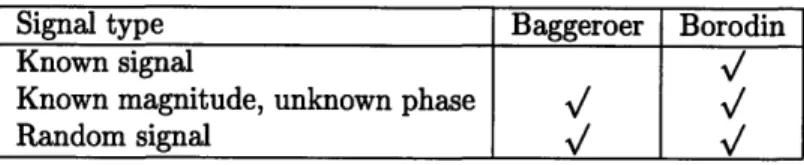
followed this idea. Three different source signal types were considered by both authors (see Ta-ble 1.1).

Signal type Baggeroer Borodin Known signal

Known magnitude, unknown phase / /

Random signal

/

/

Table 1.1: Signal types considered by Baggeroer and Borodin.

was not representative of true ocean conditions, but was used to demonstrate the mathematical method. Had Baggeroer considered this type, his signal model would have been modified to set b(f) to 1 and S,(f) to the source signal. The second type of signal (known magnitude, unknown phase) was a better representation of the type of signal used with OAT. The phase was unknown due to the difficulty of obtaining the exact propagation distance between the signal source and receiver. Candidate signal types in this category included M-sequences and FM slides. Implementation of this signal type was accomplished in Baggeroer's model by setting S,(f) to the signal, and b(f) to an unknown scalar random variable.

The final class of problems focused on a source signal which was a random process. This type of signal was typically found in applications of matched field tomography and source localization. In order to apply Green's Function as a filter on the signal, one assumed the signal was a stationary random process in the wide sense and used the Wiener-Khinchine theorem. [22] It was implemented in the signal model by setting S,(f) to 1, and assumed b(f) was a random variable with a power spectral density of Sb(f).

Borodin approached the CRB derivation problem by first obtaining a Maximum Likelihood (ML) estimator. [23, 24] With enough data the ML estimator has been shown to be both unbiased and efficient[19]. From the model of the received signal, one obtained a probability density function (PDF) which had the unknown quantities to be estimated as nonrandom parameters. This PDF was differentiated with respect to the unknown parameters, and set to zero. Then the unknown parameters were solved for. The covariance matrix produced by the ML estimator was asymptotically equal to the Fisher Information Matrix used to determine the CRB.

1.3.2 Applications of CRB to MFT and OAT

Borodin published a second paper which applied the CRB derivations to OAT [25], His objective was to show what information was required in order to obtain varying levels of precision with OAT. He first dealt with the case of estimating "global inhomogeneities," that is, reconstructing the

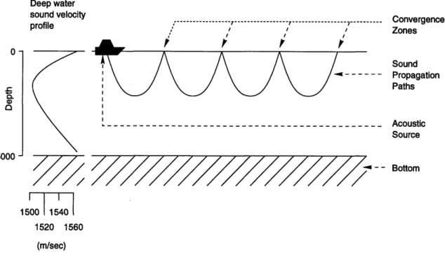
ocean environment with precision less than the typical convergence zone distance. A typical deep ocean environment refracts downward propagating sound upward. After tens of kilometers, sound converges again at the surface (hence the term, "convergence zone") is reflected, and propagates again (see Figure 1-7). Borodin proved one needed to measure only the arrival times of normal

Deep water

sound

/

---

Bottom

15

00 15401

Figure 1-7: Convergence zone scenario. In deep water ocean environments, sound is refracted to the surface, providing "convergence zones" of acoustic energy.

waves to successfully reconstruct the ocean environment in this manner. Only the travel times for deterministic signals (or the time differences for stationary random signals) carried information about the environment.

-Next, Borodin solved for "small-scale inhomogeneities." By applying his previous derivation for CRB to this problem, he was able to determine what data would be necessary in order to obtain tomographic resolution greater than a typical convergence zone width. There it was shown the ability to reconstruct the environment adequately depended on the location of the shadow zones. Inside the shadow zone, reconstruction failed, while outside it succeeded. In order to succeed at all depths and ranges, it was determined that several transmitters and receivers would be required, placed at varying depths and orientations. This contrasted with the typical point source transmitter and vertical line array (VLA) receiver.

Krolik and Narasimhan[26] used Baggeroer's CRB derivations to find the CRB for estimating a depth dependent temperature profile in the Pacific ocean. The environment under consideration had areas of "mesoscale variability," that is, the temperature profile differed on a scale of 100 km. The objective of ATOC was to measure the temperature profile as a whole, so these areas of variability had to be neglected. Krolik and Narasimhan decided to solve the CRB for cases where the receiving vertical array did not span the entire water column. They concluded a priori knowledge of mesoscale variations should reduce the CRB, as well as increase the number of sensors on the VLA.

Another paper submitted by Narasimhan and Krolik[27] derived the CRB for source range es-timation in a coastal New England environment. Here, they decomposed the environment into a set of EOFs, and calculated the CRB for varying SNR levels. They found the CRB diverged even when the number of propagating modes was greater than the number of environmental unknowns, unless one had a priori information on the statistics of the unknowns. Their results suggested source localization could be improved significantly from contemporary methods.

Schmidt and Baggeroer[28] took the application of CRB one step further. They analyzed a hypothetical shallow water environment, and solved for the CRB of several parameters. Schmidt focused on the coupling between different parameters, and their effects on parameter estimation. He concluded that some errors in adaptive parameter estimation algorithms can be attributed to parameter coupling.

For example, rudimentary forms of MFT typically use a grid search algorithm to find the optimal parameters for the supplied environment. One establishes a range in which to search, and the grid resolution, or spacing, for each search. If only one parameter is desired, the grid is one-dimensional. For two parameter estimation, the search grid is two dimensional, and so on. Each point on the search grid corresponds to an ocean environment with "candidate" parameters. Acoustic propaga-tion between the source and receiver is simulated using these "candidate" parameters. Correlapropaga-tion

between simulated and actual results is calculated, and plotted on an ambiguity function. The pa-rameter set (grid point) with the highest degree of correlation is assumed to be the correct papa-rameter set.

Adaptive forms of MFT improve on the basic algorithm by limiting the search grid range, and adjusting the grid resolution to recursively focus on solution points. Ideally, this allows one to efficiently find the peak of an ambiguity function. Unfortunately, without appropriate a priori information, an adaptive algorithm incorrectly limits the grid size, and converges on the wrong peak. Schmidt suggested if consideration of parameter coupling were included in adaptive search algorithms, the accuracy of peak localization would improve considerably.

1.4

Summary

This chapter has served as a review in basic underwater acoustics, normal mode propagation, and Green's Function. Armed with this knowledge, the concepts of Matched Field Processing, Matched Field Tomography, and Ocean Acoustic Tomography and their relationships to underwater acoustics were explained. Additionally, a review of current literature in the application of the Cramer-Rao lower bounds to these items was presented.

The next chapter shifts emphasis to the CramBr-Rao bounds themselves. It starts by describing nonrandom parameter estimation, then explains the CRB applied to a scalar parameter. From there, the application of the CRB to MFT and OAT is expressed in mathematical form. These two chapters provide background for Chapter 3, which explains the simulations carried out in this thesis.

Chapter 2

Theory and Formulation

This document assumes the reader is familiar with the concepts of parameter estimation of non-random quantities. Kay[24] has written an excellent tutorial on estimation theory; this can be used by the reader as a reference. Other supporting sources of information are Papoulis[23], and van Trees[19]. These texts review the concepts of estimation, as well as the mechanics involved in deriving and implementing nonrandom parameter estimators.

2.1

Cram6r-Rao Bound

The Cram6r-Rao lower Bound (CRB) finds the theoretical absolute lower bound on the covariance of an unbiased estimator. It does not attempt to find the actual Minimum Variance, Unbiased (MVU) estimator; but an estimator whose variance equates the CRB would be the MVU estimator. For a scalar parameter, the CRB can be found by evaluating

Aa(a) >- 1 (2.1)

J- (a)

and

aJ4(a) = E

(

lnp(Y;a))2

I

,

(2.2)

where a is the quantity to be estimated,

y is observed data used as input to the estimator, p,(Y; a) is the probability density function of observed data y,

taking into account parameter a,

Jy (a) is the Fisher Information quantity,

and Aa (a) is the variance of the estimated quantity, &.

Examination of equation 2.2 shows the derivative is taken with respect to the parameter, instead of the observed quantity. Most probability density functions (PDF) are plotted with respect to an observed quantity. It is intuitively easier to take the derivative with respect to the parameter if the PDF were plotted with the parameter as the independent variable. The logarithm in equation 2.2 may not be possible to evaluate at all instances of a. If the argument of the logarithm were undefined or zero, it would not be possible to calculate the CRB.

2.2

Mechanics of the CRB

Although equations 2.1 and 2.2 are adequate for calculating scalar CRB, extensions to the equa-tion exist for calculating the CRB of several parameter at once, from sets of observed data. While the details of deriving the CRB equation are beyond the scope of this thesis, the resulting formulas,

and

[Jy(a)]ij = -E [02 lnpy(Y; a)]

where

and

(2.3)

(2.4)

a= [al a2 ... a ],

Y is a column vector of observed data for use as an input to the estimator: Y = [yl Y2 ... YN]T,

py(Y; a) is the probability density function of observed data Y, taking into account parameter vector a,

Jy (a) is the resulting Fisher Information Matrix,

A&(a) is a matrix which describes the variance and covariance of the estimated parameters,

are provided for reference. If one assumes the noise component the observed signal to be Gaussian in nature,

y - N (p(a), K(a)) ,

(2.5)

then the properties of the distribution are exploited to better determine the CRB. Knowing a Gaussian distribution can be completely characterized by its first two moments, the CRB expression,

[Jy(a)]i _{(a) t K-'(a)}

. (

+ 1 Tr K-'(a) K-'(a)> K (a

2 1

a

i oaj

(2.6)

can be rewritten in a simpler form. Again, the details of deriving the CRB are excluded [24], but equation 2.6 is provided for reference. This equation assumes a real mean and variance. Complex parameters can be considered by removing the factor of 1/2 from the expression.

2.3

Application of the CRB to MFT and OAT

This thesis focuses on calculating the CRB for several parameters of the ocean environment. Prof. A. B. Baggeroer derived the original equations for calculating the CRB applied to MFT and OAT [29]. This derivation is summarized below.

In order to derive an equation for the Cram6r-Rao bounds (CRB) applied to both MFT and OAT, one must start by making assumptions about the characteristics of the received signal. First, and most importantly, one limits the analysis to zero mean signals which are embedded in Gaussian white noise. Next, one allows for complex statistics in the Gaussian distribution. This allows one to solve for elements of the Fisher Information Matrix (FIM) using

[Jr(a)]ij = Tr [Kr- (a)0 r(a Kr-'(a) aj (2.7)

a simplified version of the CRB equation. The input of Equation 2.7, K,(a) is a standard covariance matrix formed by taking the expected value of the observed input, R, multiplied by its complex conjugate,

Kr(a) = E [RRt]. (2.8)

One solves the CRB for a specific signal bandwidth. This requires one to incorporate a frequency dependence into the CRB equation. This is handled by the R vector, which contains the received signal for each sensor and frequency of interest.

The signal at the receiver array is acquired initially in the time domain. In order to convert it to the frequency domain, a periodogram type of spectral estimation is assumed. This is performed on the time-domain signal at each receiver. The result is a spectral estimation of the received signal at each sensor.

One starts the spectral estimation process by taking the zero mean received signal at sensor n, rn(t), and calculating its short time Fourier Transform,

Rn(f

ITo)

Next, one estimates the received signal Power Spectral Density (PSD) using the periodogram method. The result is an estimate of the power spectral density of the received signal for sensor n, during observation time T,.

Recall the correlation function for a time domain signal,

E[rn(t)r(

)]

One incorporates Equation 2.10 to estimate the PSD,

E [Rn(f₁lTo)R(f 2 To)] -= /2 E [rn(tj) r 2)]e-j 1(f2 f(tit -f2t2)dt ldt2,

n f0-/2 f-

+0

JToej2r(v-f

)tIdt1

(2.11)

S-f

ej2f(v-f2)t2dt

dv,

I

To

-To/2

fl)

}sinc

d.

Next, one assumes Sr(v) is "smooth" in intervals of -L. If Sr(v) were relatively constant, it would

be taken outside the dv integral,

E[R(fi|To)R(f

ITo)]

SSr(f) sinc [2(fi -

f2)

If fi were equal to f2, then Parseval's theorem would be used to reduce the expression,

S()(2.13)

E [R,

(fl To)R~L

(f

To) ]

=

(2.13)

to a single term. This formulation can be extended to the vector case, where one has a set of N sensors receiving a signal, R. The power spectral density estimate, Sr, would be a matrix instead of a scalar. It includes cross terms describing the frequency correlation between receiving sensors. The vector form,

E [R(f ITo)Rt(f ITo)] = (f) (2.14)

At this point, a notational change must be made to conform with Prof. Baggeroer's original derivation. In the equations above, it is obvious a bias of 1/To was introduced into the spectral density estimate. In order to obtain the "true" estimate, the bias must be multiplied out. Prof. Baggeroer's formulation assumed the bias to be incorporated into Sr(f), eliminating the need to show a division by To. However, he factored the bias out by multiplying his representation of S,(f) by To,

Kr(f) = ToSr(f). (2.15)

The Kr(f) matrix represents the spectral covariance matrix of the received signal. It is this expression which is used in the Gaussian CRB equation listed above.

2.3.1

Matched Field Tomography

The next step is to examine the structure of the received signal. For MFT, the received signal

R(f, a) = b(f)Ss(f)G(f, a) + N(f, a), (2.16)

where: _{R(f, a) = received signal vector, evaluated at frequency f,}

b(f) = random process with power spectral density equal to the source, Sb(f)

S,(f) = assumed to be 1 for MFT case,

G(f, a) = Green's function,

and N(f, a) = noise vector,

is broken down as a combination of signal and noise. Taking the expected value of the received signal squared, and adjusting for the spectral density estimate bias results in

E[R(f To)Rt(f To)] = ToSb(f)G(f, a)Gt(f, a) + ToSn(f), (2.17)

the receiver covariance matrix. Note the formation of the spectral covariance matrix is for a single frequency only. In order to calculate the CRB, all frequencies in the selected bandwidth of interest

would be needed. However, MFT assumes the received signal is uncorrelated across frequency. This allows one to process the result on a frequency by frequency basis.

By arranging the received signal vector, R =

R (filT

)

R

(f

To)

RN(fi

IT

)

RI (f21To)

R

(f2T

)

RN(fMITo)

(2.18)

in such a manner that it spans M frequencies and N receiver sensors, one can process all frequencies and receivers of interest simultaneously. Solving for the spectral covariance matrix,

K,(a) = Sb(fl)G(fl, a)Gt(fl, a) 0 ... 0 0 Sb(f 2)G(f2,a)Gt(f2,a) ... 0 To 0 0 . Sb(fM)G(fM,a)Gt(fM,a)

S.(fl)

0

0

o

results in a block diagonal form.

Referring back to the Gaussian CRB equation, both the inverse and derivative of K, (a) are block diagonal matrices. Multiplication of four block diagonal matrices together yields another block diagonal matrix, and the trace of a block diagonal matrix is equivalent to the sum of the trace of the submatrices. With these assumptions, the CRB equation,

[Jr(a)]ij = Tr [Kl '(fma)Kr (fm (fm,a) OKr (fm, a) (2.20)

m=1

can be re-written in a more computationally tractable form. Using Woodbury's identity, both the receiver covariance matrix inverse,

K '(fm,a) = {S _(fm) - Snl(fm)G(fm,a) To x [Gt(fm,a)Sn'(fm)G()G(fm,a)+ Sb(fm)-1 - 1G t_(fm,a)Sn (fm) (2.22) 1 S() (fm)G(fm, a)Gt( (fm, a) S(fm) To Gt(fm, a)S '(fm)G(fm,a) + Sb(fm)-1

and its derivative,

Krf, a) ToSb(fm) _G ( ,a)Gtfma) + G(fm, a) G (fm,a)

aa IJ~i a

can be written. To aid in term simplification, four quadratic identities,

d2(fm,a) = Gt(fm,a)Snl(fm)G(fm,a),

S(fm,

a)

are introduced. Each quadratic term has significance in the equation. The Sb(fm)d2(fm, a) term

is the Signal to Noise Ratio (SNR) for Green's function in additive noise. li(fm, a) is a measure of the mean of the parameter sensitivity under additive noise conditions, while li,j (fm, a) measures the convexity of parameter sensitivity. At low SNR,

y(fm,

Sb (fm)d2(fm, a) term becomes large, lowering -(fm, a).

With this information, the Fisher Information Matrix (FIM) equation can be expanded,

[Jr(a)]i,j =

M TS ) S[(fm)G(fm,a)Gt(fm,a)Sn'(fm)

T S;

r

(sm)

_-

-

_+T]

₎

E d2(fm,a) + Sb(fm)

X Sb(fm) [G(fm, a) O(fm,a) G(fm,a)(fm, a)]

d2(m,

a )

I

aBaj

iaj

(2.28)

as the observation time, To, cancels out. After some algebra, the quantity inside the summation can be expressed with 16 individual terms, which combine to form

[Jr(a)]i,j

=

ES(fm)7(fm, a) Re

_{[d2(f,,a)li,j(fm,a)}

-

_{li(fm,a)t(fm,a)]}

- y(fm,a)Re[li(fm,a)] Re [lj(fm,a)]}.

(2.29)

Finally, the summation can be converted to an integral. One must multiply and divide by Afs, the inter-frequency spacing. The inverse of Af, is equal to the sampling time, T,. Provided Af, is small,

[Jr(a)]i,j -Tf, S (f )y(f,a) {Re [d2(a)ij(f , a) _{d ra)(f,} - 1(f, _a)

- t(f, a)Re [l1(f, a)] Re [Ij (f, a)]} df,

(2.30)

with

d

(fm,a)

=

G

(fm,a)S (fm)G(fm, a),

2

(f, a) =

1 +

_{1 + Sb(fm)d}

2

_(fm,

_a))'

li(fm,a) = Gt(fm,a)S; (fm) OG(fm,a)

Bai

and ij(fma) = c9Gt(fm, a) )G(fm, a)

aand (fa)

l(f9m)

a

Bai Baj

a simplified equation for the CRB applied to Matched Field Tomography results.

2.4

Ocean Acoustic Tomography

Ocean Acoustic Tomography (OAT) differs from MFT in its treatment of the received signal. While MFT operates on incoherent signals, OAT is better suited for processing broadband signals which are coherent across a given frequency range. The received signal

R(f,a) = b(f)Ss(f)G(f,a) +N(f,a), (2.31)

assumes both a signal and noise component. b(f) is a scalar random variable with variance ab. Both exact distance and attenuation over the propagation channel cannot be known exactly; b(f)

allows for random phase and amplitude at the receiver. The source signal, S,(f) is deterministic, as is Green's function G(f, a). The noise vector, N(f, a), is Gaussian in nature, and is uncorrelated across both space and frequency.

Taking the expected value of the received signal squared, and factoring out the spectral estimation bias,

SH(fl, f

)

S

(fl)S;(f

)G(fi,a)Gt(f

,a)

and

E[R(fi|To,a)Rt(f2ITo, a)] = arSH(fl, f2) +T oSn(fi, f2)

results in the OAT receiver covariance matrix.

Estimation of Ub does not rely on an observation time; ab is assumed to be a known quantity. Matrix computation is simplified if To is present in both terms of Equation 2.33, so a new variable, a2, = a2/T, is introduced into the receiver covariance matrix,

E[R(fiITo, a)Rt(f 2To, a)] = C TToSH(fl, f2) + ToSn(fl, f2). (2.34)

OAT assumes coherency across a frequency band. The resulting power spectral covariance matrix is not block diagonal (as in the MFT case). Because of this, the problem cannot be broken down and solved for single frequency increments; the entire frequency range of interest must be considered at the same time.

Assuming a received signal vector arrangement as in Equation 2.18, one arrives at a spectral covariance matrix, Kr(a) = abT To SH(fl, fl) SH(f2, fl) SH(fM,

f)i)

which is not block-diagonal. The next step is solving for the matrix inverse of K,(a) and derivative (2.32)

(2.33)

with respect to a2. Again, since K,(a) is not block diagonal, the problem needs to be reformulated

slightly.

Consider combining the source signal and Green's function into one vector,

H(a) =

Ss(f

)G(fi, z

,

a)

S,(fl)G(f

,

z

,

S,(fM)G(fM,zN,a) )

Then, rewrite the received spectral covariance matrix,

K,(a) = To [S, + H(a)aoTHt(a)], (2.37)

into a simplified form. Using Woodbury's identity, the inverse of the receiver covariance matrix,

Kr1(a)

1 S - S

-'H(a)

1

[Ht(a)S'IH(a)

+o~']

Ht(a)S.'}

Ht(a)S,1H(a)Ht ()+

H•bT

=

aTTo [H(a)a

(

)

Substituting these expressions into Equation 2.7 yields another multiple term equation, with the observation time, To, canceling out,

S, H(a)Ht(a)S

'1

2

Ht(a)Sn H(a) +

Ub-[H(a)oHt ( 0aj

8Ht(a) + H(a)

+ai + ai

+

_{H(a Ht (a)]}

Attention should be focused on one of the the quadratic terms in the denominator of Equation 2.40. oK,(a) oai (2.39) Jij (a) =

'bTTr

{

Ht(a)Sn-H(a)

-It(a)]

(2.40)

TO I

n