HAL Id: hal-02562811
https://hal.archives-ouvertes.fr/hal-02562811
Submitted on 5 May 2020HAL is a multi-disciplinary open access archive for the deposit and dissemination of sci-entific research documents, whether they are pub-lished or not. The documents may come from teaching and research institutions in France or abroad, or from public or private research centers.
L’archive ouverte pluridisciplinaire HAL, est destinée au dépôt et à la diffusion de documents scientifiques de niveau recherche, publiés ou non, émanant des établissements d’enseignement et de recherche français ou étrangers, des laboratoires publics ou privés.
Scanless two-photon excitation with temporal focusing
Eirini Papagiakoumou, Emiliano Ronzitti, Valentina Emiliani
To cite this version:
Eirini Papagiakoumou, Emiliano Ronzitti, Valentina Emiliani. Scanless two-photon excitation with temporal focusing. Nature Methods, Nature Publishing Group, 2020, �10.1038/s41592-020-0795-y�. �hal-02562811�
1
Editorial Summary:
This Review discusses temporal focusing microscopy and its applications in neuroscience for imaging and optogenetic activation.
Scanless two-photon excitation with
temporal focusing
Eirini Papagiakoumou, Emiliano Ronzitti and Valentina Emiliani Wavefront-Engineering Microscopy Group, Photonics Department, Institut de la Vision, Sorbonne University, Inserm S968, CNRS UMR7210, Fondation Voir et Entendre, 17 Rue Moreau, 75012 Paris, France
Summary
Temporal focusing, with its ability to focus light in time, enables scan-less illumination of large surface areas at the sample with micrometer axial confinement and robust propagation through scattering tissue. In conventional 2P microscopy, widely used for the investigation of intact tissue in live animals, images are formed by point scanning of a spatially focused pulsed laser beam, resulting in limited temporal resolution of the excitation. Replacing point-scanning with temporally focused widefield illumination removes this limitation and represents an important milestone in 2P microscopy. Temporal focusing (TF) uses a diffusive or dispersive optical element placed in a plane conjugate to the objective focal plane to generate position-dependent temporal pulse broadening which enables axially confined multiphoton absorption, without the need of tight spatial focusing. Many techniques have benefitted from TF, including scan-less imaging, super-resolution imaging, photolithography, uncaging of caged neurotransmitters and control of neuronal activity via optogenetics.Introduction
“It appears that a nonzero probability exists that an excited atom divides its excitation energy into two photons, whose energies in sum prove to be the excitation energy but are otherwise arbitrary… Additionally, the reversal of this process is considered, namely, where two photons whose frequency-sum equals the excitation frequency of the atom co-act to excite the atom”1. With these sentences, Maria Göppert-Mayer, who was awarded the Nobel prize in Physics in 1963, predicted the process of 2P absorption in 1930 (Box 1).Crucially, the probability of co-action by two photons exhibits a quadratic dependence on the photon density. Therefore, maximizing photon density at the focus by shaping the excitation beam generates axially confined absorption, which can be used for optical imaging with inherent 3D resolution. The discovery of Maria Göppert-Mayer thus marked the beginning of 2P microscopy.
In conventional 2P excitation (2PE) microscopy, first demonstrated over 30 years ago2–4, axially
resolved optical imaging is achieved by 3D scanning of a spatially focused beam, which constrains the maximal volumetric imaging speed. In contrast, temporal focusing, first demonstrated in 2005 (ref.
5,6), enables scan-less axially resolved 2P imaging by temporally concentrating the photon density at
the focal plane. Despite its relatively recent emergence, temporal focusing has already found applications in scan-less imaging, optogenetic neuronal stimulation, super-resolution imaging and
2
multiphoton microfabrication, marking a new era in 2P microscopy. Here we review significant steps in the history of TF, from the prediction of Maria Göppert-Mayer of 2P absorption to the first demonstration of TF. We present the principle of temporal focusing, outline important optical design constraints and describe the main approaches which have benefitted so far from this technique.
From point-scanning to scanless 2P-microscopy
After the prediction of Maria Göppert-Mayer, it took 30 years to experimentally demonstrate 2P absorption. The reason is that the low probability of the 2P absorption and the necessity of using “light of two narrow frequency ranges...with equal directions of propagation and equal polarization”1 required the development of high-intensity, monochromatic light sources. The development of the first ruby lasers in the 1960’s enabled the experimental confirmation of Göppert-Mayer’s prediction of the quadratic dependence of 2P absorption by organic molecules2, cesium vapor3 and inorganiccrystals4. A further 30 years later, Winfried Denk, James Strickler and Watt Webb recognized that “The
quadratic dependence of signal on excitation intensity is responsible for another advantage of two-photon excitation: it provides an optical sectioning effect, …”7. Indeed, spatial focusing using an optical
lens creates an axial gradient in photon density, with its maximum at the focal plane. In this configuration, the probability of 2P absorption decreases axially from the focal plane, resulting in intrinsic optical sectioning without the need of a pinhole, which is required for single-photon (1P) confocal microscopy. Furthermore, 2P absorption using dye molecules and 2P scanning microscopy in biological specimens could be demonstrated with an infrared, femtosecond-pulsed laser7. These developments heralded a new era for 2P microscopy in biological research with an ever-increasing list of applications ranging from structural and functional imaging to photolysis and optogenetics8–13.
Since then, refinements in the implementation of 2P scanning microscopy have increased acquisition speed to rates of tens of Hz, for instance by use of resonant scanners14, inertia-free
acousto-optic deflectors15,16 or beam multiplexing in both space and time17,18. In addition,
technological developments such as low-repetition rate lasers, adaptive optics and endoscopic GRIN lenses have increased the penetration depth19–22. Methods based on point spread function
engineering and/or custom designed focusing optics and multi scan heads were applied to increase the imaging volume23–27. Despite this progress, 2P microscopy had remained a scanning approach
with fundamentally limited temporal resolution.
This limitation was overcome in 2005 with the demonstration of scanless, depth-resolved microscopy using the principle of TF5,6,28. Here, a “temporal focusing” element, a “time lens”,
temporally focuses the photons of a weakly spatially focused beam at the objective focal plane and reduces the temporal density of photons at out-of-focus planes, which decreases the probability of 2P absorption. The rapid reduction of 2P absorption away from the focal plane results in optical sectioning (Box 2), despite the weak spatial focusing. This strategy enables simultaneous, scanless, depth-resolved imaging across large areas, as first demonstrated in a Drosophila egg chamber5. TF is
also compatible with other coherent imaging modalities, such as third harmonic-29,30 and
sum-frequency generation31, and it can achieve super-resolved multi-plane imaging32 and fast, in vivo
functional imaging33,34.
In addition to its application in imaging, TF has had a tremendous impact in optogenetics. The combination of TF with weakly focused (low-NA) Gaussian35 or phase-sculpted beams36,37 has
facilitated efficient 2P neuronal control with micrometer axial resolution and millisecond temporal resolution both in vitro and in vivo38. Temporally focused light-pulses have been also applied to
micromachining39–41, tissue laser ablation42 and 3D lithographic microfabrication43. More recently, TF
imaging has been combined with 3D holographic optical tweezers for depth-resolved 2P imaging of trapped objects44.
3
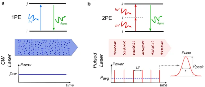
Figure 1ï Schematic representation of 1P and 2P excitation processes. a, Jablonski diagram of 1PE (top), and representation of the excitation beam (middle) with the corresponding power, PCW,
(bottom) of a continuous wave (CW) laser. b, Same as a, for 2PE. The excitation beam is formed by a laser generating pulses with duration τ, distributed at a repetition rate f. Each pulse is characterized by the peak power, Ppeak=!", i.e. the amount of energy E contained in it. The average power, Pavg, of the
excitation beam is the rate of energy flow averaged over one full period (T=1/f) 𝑃#$%=!
&= 𝐸𝑓
(bottom). Dots in the beams represent photons.
Box 1: Multi-photon excitation
Two-photon absorption, as schematized in Fig. 1, is the process that promotes an atom or molecule from a ground (S0) to an excited state (S1) through the “quasi” simultaneous absorption of two
photons, of frequency ν’ and ν’’ through an intermediate very short-lived (τ'»10-16 s)† quantum or
“virtual” state45. The number of absorbed photons per molecule per time unit, 𝑛()#, is the product of
the number of absorbed photons at each intermediate transition, that is, ∝ 𝐼(𝛿
',+𝛿+,,τ', where I is the
illumination intensity and 𝛿',+𝛿+,, are the single-photon (1P) cross-sections (~10-21m2) (Ref. 45)
accounting for the transitions i,j and j,k, respectively (Fig. 1). The factor 𝛿',+𝛿+,,τ' is usually indicated as the 2P cross-section, 𝛿(-, of the molecule and falls in the range of 10-58 m4s. Under time-varying illumination intensity 𝐼.(𝑡), the time-averaged number of photons absorbed per molecule is given by 〈𝑛()#(𝑡)〉 = 0/ 011 ( 𝛿()𝑔〈𝐼.(𝑡)〉(, (1) Where ℎ is the Planck constant, c the speed of light, λ the excitation wavelength. The dependence of the 2PE signal on the photon temporal distribution is described by the term 𝑔 =〈3!"(5)〉 〈3!(5)〉" (the second-order temporal coherence of the illumination source). For an ideal continuous wave (CW) laser 𝑔 = 𝑔18= 1, while for a pulsed laser of pulse duration t and repetition rate f (Fig. 1b), 𝑔 = 𝑔)9 = 𝑔)";: where 𝑔) is a correction factor accounting for the pulse shape, which for a mode-locked laser is 0.66 (Ref. 46). Since 𝑔)9 is typically 105 times larger than 𝑔18, it follows that using a CW laser would require
orders of magnitude higher average power to achieve the same fluorescence signal, thus the use of pulsed lasers for fluorescence microscopy is crucial. For example, in the case of GFP molecules having 𝛿(-≈ 21 ∙ 10<=> m4s, reaching saturation (i.e. the situation where each molecule in the illumination hv λem j i Power
4
volume absorbs two photons per pulse: 〈?"#$(5)〉
; = 2) would require 〈𝐼.(𝑡)〉 ≈ [email protected]/ m2s. This, for
a pulsed laser of pulse 𝜏 = 100 𝑓𝑠 and repetition rate of 80 MHz focused to a surface A (𝐴 = 𝜆(⁄𝜋𝑁𝐴(, NA = 0.8 and l = 900 nm) corresponds to a saturation power of ≈ 80 mW. Using a CW laser
to generate the same flux of photons would require a √10= higher power, i.e. ≈ 25 W. For comparison,
saturation in the single-photon excitation case with excitation wavelength, λ = 450 nm, would only require ~3 mW.
Generalizing to m-photon absorption processes, the number of photons absorbed per time, per molecule, is ∝ 𝐼A𝛿
A- where 𝛿A- is related to the transition probability and the lifetime of each
intermediate state (i.e., 𝛿A-≈ ∏ 𝛿','B:× ∏A<:Δ𝑡+ +C: A<: 'C. ), and Eq. 1 becomes, 〈𝑛A)#(𝑡)〉 = 0/ 011 A 𝛿A)𝑔(A)〈𝐼 .(𝑡)〉A, (2) where 𝑔(A)=〈3!%(5)〉 〈3!(5)〉% is the m th-order temporal coherence of the excitation beam, which for a pulsed
laser is given by 𝑔)9(A) = 𝑔)(A)(";):%&' , with 𝑔)(A) a function of the pulse shape.
†According to the Heisenberg energy-time uncertainty principle the lifetime of an energy state is τ=(h/4πΔΕ), with h = Planck constant and ΔΕ the energy difference between the virtual state and the nearest eigenstate. A virtual state excited with an excitation wavelength of 900 nm excitation will therefore have a life time of τ ≈2.5×10⁻¹⁶ s. Box 2: Optical Sectioning in spatial and temporal focusing High-resolution 3D imaging requires optical sectioning, i.e. the ability to discriminate between in-focus and out-of-focus planes of the sample. As a consequence of the non-linear dependence of 2P absorption on the excitation photon density, any spatial or temporal confinement of excitation photons can be used to achieve optical sectioning. According to Eq. 1 (Box 1), the fluorescence signal, Se, produced by 2P excitation with a pulsed laser beam with a spatially varying illumination profile I0 (r,z,t) is given by45: 𝑆D(𝑟, 𝑧, 𝑡) ∝ : "; 〈𝐼.(𝑟, 𝑧, 𝑡)〉 (, (3)
with 𝑟 = K𝑥(+ 𝑦(. For collimated incident Gaussian beams with beam waists smaller than the
objective aperture, the intensity distribution 𝑆D(𝑟, 𝑧, 𝑡) in the perifocal region of the objective lens can be approximated as 𝑆D(𝑟, 𝑧, 𝑡) ∝ : ";∙ P 〈-(5)〉 E8"(F)𝑒 <)"(+)"(" R ( 𝑤(𝑧) = 𝑤.T1 + UGFF -V ( 𝑧H =E8!" / , (4)
where P is the incident power, 𝑤.~(IJ/ is the beam waist at the focal plane (z=0) and 𝑧H is the Rayleigh
range of the focused beam. According to this equation, the axial resolution (defined as the FWHM of 𝑆D along the optical axis (r=0)) is Dz = 2𝑧H (Fig. 2a) and the optical sectioning (defined as the axial dependence of the integrated intensity at each scanned plane47,48) is proportional to : E8"(F) , which falls off as ~1/Δ𝑧( for Δz > z R. Since w(z) is inversely proportional to the numerical aperture (NA) of
the focusing lens, scanning with strongly spatially focused beams (or high-NA beams) enhances optical sectioning.
5
Increasing the temporal resolution of 2P microscopy requires using scanless strategies by means of low NA-beams corresponding to a large (50-100 µm diameter) illumination spot at the focal plane. However, increasing the lateral spot diameter also deteriorates the 2P optical sectioning, as all planes in the large excitation volume, equally excited, equally contribute to the collected signal, i.e.
: E8"(F)𝑒
<)"(+)"("
≈ 𝑐𝑜𝑛𝑠𝑡. (Supplementary Fig. 1).
In this condition, optical sectioning can be recovered by taking advantage of the 2P absorption dependence on 1/τ. This is achieved by generating a “temporally focused” beam with an axial dependent pulse broadening 𝜏(𝑧), where the laser pulse is stretched away from the focal plane, compressed as it travels towards it and stretched again beyond it (Supplementary Fig. 1b). Large temporally focused beams at the sample plane are technically achieved by illuminating the objective back aperture with a thin line (Fig. 2b) generated by spatially separating the spectral components of a short pulse with a grating (Fig. 3). In this configuration, the axial pulse dependence is given by49: 𝜏(𝑧) =(√(9?( L T1 + F. F/ GF" GF"BF.F-, (5) where 𝑧M =(;01" ,!N", 𝑧H = (;01" ,!(N"BO"L"), 𝑧P = (;01" ,!O"L" are the corresponding Rayleigh length for the spatial, the spatial and chirped (spatiotemporal) and the chirped focusing parts of the beam, respectively, √2𝑙𝑛2𝑠 is the FWHM of each monochromatic beam at the objective back aperture, k0 the wavevector of the central frequency of the pulse, a a constant proportional to the grating groove density and the focal length of the collimating lens, W the full width at half maximum of the frequency spectrum of the pulse and fob the objective focal length. Notably, 𝛼𝛺 is the linear spatial chirp at the objective back
aperture, i.e. the extension of the illumination at the objective back aperture in the chirping direction (where the wavelength components are dispersed). For temporally focused illumination, the intensity in the perifocal region may be written: 𝑆D(𝑟, 𝑧, 𝑡) ∝: ; Q (√(9?(01 + F. F/ GF" GF"BF.F-1 <'" 〈𝑃(𝑡)〉( . (6) As typically 𝑠 ≪ 𝛼(𝛺(, 𝑧 H ≈ 𝑧P and 𝑧M ≫ 𝑧H, Eq. (5) can be approximated as 𝜏(𝑧) ≈(√(9?( L T1 + GF" F-" (7) such that Eq. (6) may be written: 𝑆D(𝑟, 𝑧, 𝑡) ∝ : "!;01 + GF" F-"1 <'" 〈𝑃(𝑡)〉(, (8) where 𝜏.=(√(9?( L is the pulse length at z = 0. According to this equation, the axial resolution is Dz = 2√3𝑧H and the optical sectioning scales as 1/t(z) and falls off as ~1/Δ𝑧 for z >zR . Similarly to spatial focusing, stronger temporal focusing (i.e. the smaller the ratio f2/𝛼(𝛺() results
in stronger axial confinement of the 2P signal. It is worth noting that Eq. (8) is equivalent to the expression for the 2P fluorescence signal that one would obtain in conventional line-scanning microscopy using a constant pulse duration 𝜏., corresponding to an optical sectioning that also scales as ~1/Δ𝑧 for Δz > zR (Refs.5,6,13,49,50).
6
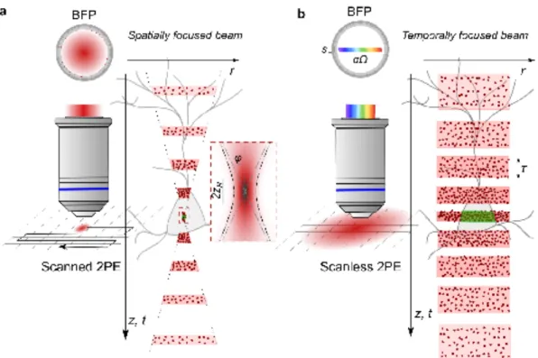
Figure 2ïAxial propagation of spatially and temporally focused beams. a, Left, Schematic representation of scanned 2PE with a spatially focused beam and corresponding beam intensity distribution at the objective back focal plane (BFP). Right, representation of the spatio-temporal distribution of photons for spatial focusing of illumination (red dots and pink bands correspond to photons and laser pulses, respectively). Photon density increases at the focal plane because of spatial confinement of photons. The Rayleigh range, 2zR and the maximum illumination angle, φ (NA=nsinφ,
where n is the medium refractive index), are shown in the inset. b, Same as in a for scanless 2PE with a temporally focused low-NA beam. αΩ is the linear spatial chirp and √2𝑙𝑛2𝑠 the FWHM of each monochromatic beam. Photon density increases at the focal plane because of temporal confinement of photons, i.e. the width of illumination pulses gradually gets shortened by getting closer to the focal plane.
Temporal Focusing: experimental realization and axial resolution
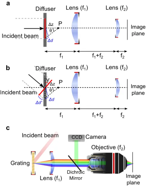
In one of the first implementations, TF was achieved using a thin scattering plate (diffuser) conjugated to the sample plane through a telescope of lenses, where the second lens was the microscope objective. The diffuser was used to scatter each ray of the incident pulsed beam, of pulse duration t, in different directions5 (Fig. 3a). For the two paths shown in Fig. 3a, the illumination time of a point Pat a distance Δz from the diffuser is 𝜏(𝑧) =GFR(1SNT)1 &'<:U, showing that 𝜏(𝑧) increases as a function of Δz, resulting in position dependent pulse broadening in the sample volume. Introducing an angle γ between the diffuser and the optical axis introduces larger differences in pathlength for rays arriving at a given position P (Fig. 3b; Supplementary Note 1), and therefore more efficient pulse broadening. Ultimately, in order to maximize off-axis dispersion, the diffuser was replaced by a blazed grating, resulting in the most common configuration of TF: tilted illumination of a blazed grating with ~100 fs pulses (Fig. 3c)5,6. Alternative variations of TF use two parallel gratings51,52, or a digital micromirror
7
Figure 2ïExperimental realization of temporal focusing. a, Implementation of TF with a thin scattering plate (diffuser). A short pulse, τ, impinges upon the diffuser. In this geometry, each point in the image plane is illuminated for a duration τ, since, according to Fermat’s principle, all light rays emerging from the diffuser travel identical optical pathlengths and ultimately arrive at the image plane simultaneously. However, any other point P, displaced by Δz from the scattering plate, is illuminated for a longer duration 𝜏(𝑧), which depends on the different trajectories traveled by the multiple rays reaching P. The difference in the length of the optical path is Δd = 𝛥𝑧[(𝑐𝑜𝑠𝜃)<:− 1]). At
the image plane of the telescope the pulse duration is restored to its initial value, since all rays that arrive at a given point in the image plane originate from a single point on the diffuser, resulting in an illumination time identical to the original pulse duration. b, Implementation of TF with a thin scattering plate (diffuser) and tilted illumination, at an angle γ. This results in larger broadening of the pulse around the focal plane of the telescope due to the effectively increased pathlength difference (Δd+Δd’). c, Common experimental configuration: the beam impinges with a tilt upon a grating, which is aligned perpendicular to the optic axis of the microscope. The spot image on the grating is magnified at the sample plane through a telescope comprising an achromatic lens and the microscope objective. Fluorescence is epi-detected and imaged onto a CCD using a dichroic mirror. Adapted from Oron et al.5.
a
b
8
For greater intuition of widefield excitation using TF, consider an equivalent formulation of the process in the temporal domain: at each point in time the intersection between the pulse and the dispersive element is a line which is de-magnified onto the sample plane by the telescope of lenses (Supplementary Video 1). Hence, non-linear excitation with a temporally focused beam can be considered as a line-scanning process. In contrast to line-scanning based on galvanometric mirrors, the TF line-scan occurs at higher speed (1/WXYZ M ; c is the speed of light in vacuum, M= ;'
;" the magnification of the telescope), though, as derived in Box 2, the axial resolution is constrained by the same factors. For optimal axial resolution, the back aperture of the objective, of diameter D, must be filled in the chirped direction (D = 𝛼𝛺). Furthermore, the lenses telescope following the dispersive element must de-magnify the intersection onto a diffraction-limited line at the sample ( 1" N'?\≈ M/! IJ, where 𝜆. is the central wavelength of the pulse). The axial resolution can be further improved by illuminating the grating with a line perpendicular to the grating’s groove direction (line-scanning TF), for instance using a cylindrical lens28. In this configuration, the intersection of the pulse with the
grating is a point. The axial response at the sample plane is equivalent to that of 2P-point-scanning microscopy, 𝑆D~ d1 + UGFF
-V
(
e<: (Box 2), with axial resolution 𝛥𝑧 = 2𝑧H (Ref. 13). Imaging
two-dimensional areas with line-scanning TF requires mechanical scanning in one dimension28,
consequently the temporal imaging resolution is degraded with respect to the widefield case. A compromise can be reached by scanning simultaneously multiple lines, generated, for instance, using a spatial light modulator (SLM) and a lens prior to the grating55. Depending on the number of lines scanned simultaneously, the axial resolution will be bound between that of 2P-point- and that of 2P-line-scanning microscopy. Pulse shaping at the Fourier plane of the TF telescope can be used to control the temporal profile of the pulse. This can be used to correct pulse broadening (and thus axial resolution deterioration) due to dispersion, as was demonstrated by placing a one-dimension SLM at the objective back aperture30. Notably, in the case of line-scanning TF, this would require a 2D SLM.
Axial resolution can also be improved using multifocal TF which generates a set of diffraction-limited spots via an echelle grating to illuminate the grating used in TF in the orthogonal direction to that of the dispersion. In this way, the back-focal aperture of the objective is filled in one dimension due to diffraction and in its orthogonal direction due to spectral dispersion56. Implementing
structured light illumination can also improve the axial resolution based on rejection of the background noise57,58.
Temporal focusing for imaging
Following its first demonstration5, TF has been used in combination with multiple imaging
modalities, including super-resolution, fast functional imaging and 3P microscopy.
Temporal focusing in super-resolution imaging
TF has been used in super-resolution microscopy for adding axial precision to 2D super-resolved images. In their classical configuration, super-resolution methods such as PALM (photoactivated localization microscopy) and STORM (stochastic optical reconstruction microscopy) require widefield illumination to achieve fast photoconversion of large sample areas, thus losing axial resolution. On the other hand, optical sectioning enables increased signal-to-noise ratio and thus better discrimination of single molecules from the background. In order to record super-resolved images with optical sectioning, researchers have used complementary strategies, such as total internal reflection fluorescence (TIRF) and light-sheet fluorescence microscopy59.
In 2018, photoactivated localization microscopy (PALM) imaging at selected planes has been demonstrated by using a TF-Gaussian beam for photoconversion in combination with 1P widefield
9
fluorescence excitation. In this way, TF suppressed the out-of-focus background enabling imaging with a lateral resolution of 50 nm at depths up to 10 µm32.
Temporal focusing for fast functional imaging
The increased temporal resolution of widefield TF illumination compared to point-scanning illumination makes this approach particularly promising for fast functional imaging. However, its original configuration, based on conventional mode-locked lasers and camera-based detection, has important limitations. Distribution of the excitation beam across large areas strongly reduces the excitation photon density, while camera-based detection limits the imaging depth as the scattering of emitted fluorescent photons from different sample locations may contaminate one another60.
Power limitation has been overcome by reducing the illumination area to specific regions of interest and using low-repetition rate laser amplifiers. Since the 2P fluorescence signal is 𝑆D ∝
-"
"; (Box
1), an amplified laser with pulse duration typically between 200 and 400 fs and kHz repetition rate enhances 2P excitation signal relative to a commonly used Ti:Sapphire oscillator (pulse duration 100 fs and 80 MHz) by a factor of ≈ 80 for the same average power61, which also reduces heating62.
In its first demonstration, the combination of low-repetition rate lasers with holographic illumination achieved fast imaging of neuronal activity of cells in acute brain slices (3 regions of interest of 40x40 µm2, each)63. Similarly, a low repetition rate, temporally focused beam, shaped to a
widefield excitation area of 60 μm was used for volumetric calcium imaging of GCaMP5 in the head of C-elegans (1.9 µm axial confinement, acquisition speeds of 4-6 Hz)64. Imaging depth up to 300 µm was
achieved by fast scanning of a temporally focused line for calcium imaging of Fluo-4 in bioengineered neuronal tissue61.
Replacing camera-based detection with photomultiplier- (PMT) or single-pixel-detection65, can
reduce signal contamination due to scattered fluorescence. This was demonstrated by performing in vivo fast single plane functional imaging in-depth of mouse cortex using TF-Gaussian beams focused down to a 5 µm spot (10 µm axial FWHM; 160 Hz acquisition rate) and in vivo volumetric calcium imaging of a mouse cortical column (0.5×0.5×0.5 mm3) at single-cell resolution and fast volume rates
(3–6 Hz)33. Very recently, a similar approach, combined with remote focusing and spatiotemporal
multiplexing enabled volumetric (0.5×0.5×0.6 mm3) imaging at ~16-Hz volume rate34. Scan-based TF
strategies present a valuable trade-off between diffraction-limited scanning microscopy and widefield TF illumination, requiring less total excitation power and enabling greater imaging depths compared to widefield TF and higher acquisition speeds compared to diffraction-limited scanning microscopy.
Temporal focusing in 3P excitation
Recently, TF has been used with three-photon (3P) widefield excitation fluorescence imaging71,72. Compared to 2P-TF widefield illumination, 3P-TF excitation enables sharpening even further the axial resolution71. Indeed, according to Eq. (2) in Box 1 the 3PE signal is ∝ : "(F)" and therefore (see Eq. (8), Box 2) ∝ : ]:B^2+ +-_ " `. Thus, the 3P-TF optical sectioning for z >zR decays as 1/Δz2 , and the axial
resolution, Dz, is equal to 2zR, as in 2P-point-scanning microscopy. These values need to be compared
with 2P-TF illumination where the optical sectioning decays as 1/Δz and Dz is equal to 2√3𝑧H (Box
2).
Comparison between widefield 2P-TF and 3P-TF excited fluorescence on a fluorescent dye solution has shown an improvement of axial resolution by 30% and suppression of the out-of-focus excitation by a factor of ~6 (Supplementary Fig. 2)71 when imaging fixed mouse brain tissue at a depth
of 30 µm. In addition, the maximum achievable depth for widefield 3P-TF excitation by imaging quantum dots through fixed brain slices of different thicknesses has been reported as up to 800 μm with 3P excitation at 1300 nm (Ref. 72), in contrast to widefield 2P-TF excitation at 800 nm that
10
reached 400 µm. In these experiments, the maximum achievable excitation depth was characterized by collecting the excited fluorescence on the opposite side from excitation with a second objective, thus fluorescence photons did not travel through any scattering tissue. In vivo 3P-TF imaging required epi-fluorescence camera detection which limited the imaging depth to ~150 µm72 and
therefore the ultimate interest of this approach for imaging. However, widefield 3P-TF excitation can have great potential for efficient highly specific neuronal activation in depth, as in this case the cellular response can be detected with complementary methods (2P or 3P point-scanning imaging, or behavioral changes).
Box 3: Temporal Focusing and light-shaping
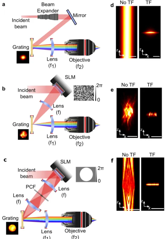
Precise illumination of neuronal somata or neuronal processes requires combining TF with laterally extended patterns with the size of a cell soma. In the simplest implementation, TF is combined with low-NA Gaussian beams to generate a 5-15µm illumination disk at the sample plane using a variable beam expander (Fig. 4a,d)33,35,66. Alternatively, axially confined shaped patterns can
be generated by combining TF with computer-generated holography (CGH) or generalized phase contrast (GPC) to enable shaped activation of a single or multiple neurons or neuronal processes.
In CGH microscopy, the SLM typically occupies a plane conjugate to the BFP of the objective. In this configuration, an image template (target) is used as the input source to a Fourier-transform based iterative algorithm (Gerchberg & Saxton algorithm (GSA)67) to calculate the interference pattern or
phase hologram at the SLM plane, that once illuminated by the laser would reproduce the target at the imaging plane (Fig. 4b)68 . For holographic illumination, the linear dependence of the axial
extension on the lateral spot size quickly deteriorates the axial resolution when illumination patterns become increasingly large, for instance when illuminating multiple neurons (Fig. 4e, left panel)69. This problem is overcome by combining CGH with TF. In this case, the dispersive grating is placed at the focal plane of the first lens, where the holographic pattern is formed. In this way the pattern projected at the focal plane of the objective is temporally focused and the axial resolution (Fig. 4e, right panel) is independent on the lateral shape extension. GPC belongs to the category of the interferometric phase visualization techniques for which the output image is obtained by the interference between a signal and a reference wave, travelling along the same optical axis70. A desired target intensity map is converted into a binary [0, π] phase map that modifies the input beam wavefront via the SLM. The beam modulated by the SLM is then focused on a phase contrast filter (PCF) which imposes an appropriate phase retardation between the on-axis focused component (non-diffracted light) and the higher-order Fourier components (Fig. 4c). The interference between these two beams generates the desired target intensity at the focal plane of a second lens (the output plane). The axial profile also reveals the interferometric character of the approach (Fig. 4f, left panel). Combination with TF is performed in this case by placing the grating at the output plane of the GPC interferometer thus recovering optical sectioning (Fig. 4f, right panel).
11
Figure 4ïTemporally focused light-shaping methods. The intensity pattern of any light-shaping method can be temporally focused by introducing a grating at the output of the corresponding system. a, In TF-low-NA Gaussian beams the grating is illuminated with a parallel Gaussian beam of the appropriate size adjusted through a beam expander. b, In TF-CGH the grating is illuminated with the holographic pattern generated by addressing the corresponding phase on the SLM (inset). c, In TF- GPC the grating is illuminated with the intensity pattern generated at the output plane of the GPC. d-f, measured x-z cross sections of 2P excited fluorescence using a thin fluorescent layer without (left) and with TF (right) for TF-low-NA, CGH and GPC beams. Scale bars: 10 µm (d), 20 µm (e, f)37.
12
Temporal focusing for 2P optogenetics
Soon after its first demonstration in imaging, TF has generated remarkable results in combination with optogenetic manipulation. Here, light-gated channels and pumps allow precise control of neuronal excitability and combined with 1P widefield illumination have enabled control over the activity of entire neuronal networks in order to unravel their role in specific behaviours.
In-depth multiscale neuronal control with single-cell precision necessitates propagating the illumination beam through scattering tissue, which is achieved by replacing 1P illumination with 2PE based on a longer excitation wavelength. In most cases, however, the small single-channel conductance of commonly used optogenetic actuators such as ChR2 (40-90 femtoSiemens73) and the limited number of channels or pumps recruited within a conventional 2P focal volume is not sufficient to bring a neuron to firing threshold or to control its inhibition. This limitation can be solved either by fast scanning of near diffraction-limited spots over the cell66,74,75, or by generating extended 2D illumination patterns (Box 3) covering the whole membrane target37,66,76. In the first case, the total illumination time for single-cell activation depends on the opsin photocycle and is typically between 5 and 70 ms74,75,77. Shorter (1- 4 ms) illumination times can be achieved using high excitation density (10-50 mW on a ~1-µm spot)77,78. Alternatively, the use of extended illumination patterns enables to illuminate the whole cell soma and therefore to reduce the excitation density (1-20 mW on a 10-12 µm spot) and the illumination time to 1-5 ms independently of the opsin photocycle. As a drawback, extended excitation patterns (generated by low-NA Gaussian beams35,66, GPC37 or CGH36,79), suffer
from poor axial resolution. This limitation is solved with TF (Box 3). Combined with a low-NA Gaussian beam, TF enables axially confined neuronal activation in brain slices66. GPC-TF allows
scanless 2P activation of multiple cells and their processes37 and demonstrated spike generation with
1-ms illumination time79. Combined with 2P imaging, photostimulation with TF-low-NA Gaussian
beams was used to manipulate task-modulated activity of individual hippocampal CA1 place cells in vivo35. Combined with fast opsins, TF-parallel illumination also enabled in vitro and in vivo optical
control of neuronal firing at high (up to 100 Hz) spiking rate with sub-millisecond temporal precision80,81. Recently, 3P optogenetic activation with large TF-Gaussian beams was also
demonstrated, by photoactivating the opsin CoChR at 1300 nm in cultured neurons72.
Temporal focusing in aberrating and scattering media
Two main factors which define the maximum penetration depth achievable with line- or widefield-TF are aberrations and scattering.
Aberrations refer to phase variations induced by imperfections or misalignments in the optical system, refractive index differences between the objective immersion medium and specimen, or optical inhomogeneity in the specimen. These aberrations can result in reduction of the axial and lateral resolution, reduction in peak intensity, or focal shifts. The way these aberrations affect the beam propagation in the sample plane can be described by the phase function at the objective BFP.
Geometries filling the BFP, such as line-TF82
, are more sensitive to aberrations compared to widefield-TF and traditional line illumination by spatial focusing83. Indeed, while in line-TF the BFP is fully
illuminated, line spatial focusing and widefield-TF only illuminate the BFP along a thin line and therefore, they are only sensitive to those aberrations corresponding to phase functions exhibiting large variations along this axis (e.g. coma and spherical aberration)83.
Scattering can affect the spatial and temporal shape of a TF beam at depths greater than the scattering mean free path length. Regarding the temporal shape, pulses on the order of 100 fs are not significantly distorted even after propagation through ~1 mm of brain tissue84, because the low-index
contrast of biological tissues causes scattering predominantly in the forward direction85 and
therefore on average the geometrical path length differences to the focus correspond to temporal delay which is much smaller than the 100 fs pulses typically used in TF.
13 The spatial characteristics of temporally focused beams are well preserved for propagation up to 6 mean free path lengths (~1200 µm) in the case of line-TF82 or 2-3 mean free path lengths (~500 µm) in the case of widefield-TF79,82,86,87. This ‘self-healing’ property of TF beams can be understood either in the frequency or in the temporal domain as schematized in Fig. 5 (Ref. 87). Furthermore, the propagation of line-TF is as robust to propagation through scattering media as diffraction-limited spots82. The self-healing effect of TF has been exploited in optogenetic stimulation experiments proving selective neuronal activation in-depth (~300 µm) using TF-shaped patterns87 and for fast, deep,
functional imaging using scanned low-NA TF Gaussian beams33,34 combined with PMT detection.
Recently, a promising approach based on TempoRAl Focusing microscopy in combination with single-pIXel detection (TRAFIX)88 has been used to create sequences of orthogonal light patterns which,
combined with de-mixing reconstructions, enabled scanless, deep imaging. These benefits are achieved at the cost of higher excitation power, compared to 2P point-scanning. For now, the acquisition time for TRAFIX is limited by the number of orthogonal light patterns (4092 or 1024) required for image reconstruction, but higher acquisition speed can be reached by incorporating a compressive sensing approach89.
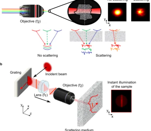
Figure 5ïTemporally focused beams passing through scattering media. a, Spectral domain representation. When a temporally focused beam travels through a scattering medium, the resulted intensity profile is smoothed out (top panel, right) because different spectral frequencies acquire different speckle patterns as they propagate through the sample to the focal plane, and these speckle patterns are averaged to form the final image (bottom panel, middle). Moreover, adjacent spectral frequencies acquire similar speckle patterns slightly shifted along the chromatic dispersion direction (bottom panel, right). The latter results in anisotropic smoothing along the dispersion direction. b, Time domain representation. Non-ballistic photons are less probable to interfere with the line that scans the sample during TF, thus they do not contribute to the formation of speckle and do preserve the original pattern. a b x y z x y x y
14
Multiplane temporal focusing
The majority of the applications described in this review, including fast 2P multiplane imaging, photostimulation or photo-polymerization, would benefit from the extension of TF to multiple axial planes. Furthermore, decoupling the plane of TF from the nominal image plane allows greater flexibility, e.g. allowing simultaneous shaped optogenetic stimulation and functional imaging on independently controlled planes in all-optical neuronal investigations.
TF-Gaussian beams can be axially displaced from the spatial focal plane by adjustments of the group velocity dispersion (GVD). The axial displacement of the temporally focused plane, ∆𝑧N0';5, is
proportional both to the amount of GVD applied, β, and to the Rayleigh range of the beam, 𝑧H: ∆𝑧N0';5= 𝛽𝛺(𝑧
H. Thus, for a given amount of GVD, a compromise has to be found between the
achievable axial shift and the axial resolution Dz=2𝑧H49,53,90,91. Several implementations of this
approach have been described, including the use of a custom dual-prism grating (DPGrism)90
(achieved ∆𝑧N0';5 < 600 µm, for line-TF with Dz ~25 µm), fast axial scanning with acousto-optic
deflectors53 (∆𝑧N0';5 >1 mm for weak TF-beams with M=3, and only ∆𝑧N0';5
=9 µm for strong TF-beams with M=60), or folded grating pair compressors using a piezo bimorph mirror91 (∆𝑧N0';5=360 µm for TF-beams of Dz = 22 µm). Remote scanning of a temporally focused spot through GVD adjustments is not compatible with temporal-focusing-shaped beams generated with CGH or GPC, since GVD only shifts the temporal but not the spatial focal plane, i.e. the image plane of CGH or GPC92. One solution to this problem is to shape the incident beam using two separate SLMs93. Here, conventional 2D-CGH was used to pattern the beam laterally, whilst a second SLM, placed in a Fourier plane following the grating, modulated the phase of the temporally focused beam with Fresnel lens profiles to introduce the desired axial shift (Fig. 6a). In this configuration, axial displacements were achieved up to 400 µm with Dz ≤ 25 µm.
The system was also used to demonstrate the generation of multiple TF holographic patterns at distinct axial planes (Fig. 6a). However, the vertical tiling of the SLM limited the maximum number of achievable planes (~6), as the reduced number of pixels in the vertical direction resulted in deterioration of the quality of the holographic spots.
This restriction was solved by using the second SLM to generate multi-diffraction-limited spots, computed by a weighted Gerchberg & Saxton algorithm94, which laterally and axially multiplexes the
excitation shape produced by an initial light-shaping module. Many possibilities of light-shaping modules exist, including low-NA Gaussian beams51,95,96, or tailor-shaped beams using CGH, GPC, or amplitude modulation methods97 . The configuration using low-NA Gaussian beams, known as 3D-SHOT, can generate hundreds of excitation spots of the size of a pyramidal cell soma (i.e. ~10-15 µm FWHM lateral size and on average ~10 µm FWHM axial resolution) in a total volume of 350×350×280 µm3 (Fig. 6b)95. A similar configuration based upon two gratings, can generate a line of multi-foci (2.5 µm in size and zR =7.5 µm) for direct laser writing on glass surfaces51.
The approach where CGH, or GPC are used to generate arbitrarily shaped patterns, known as multiplexed temporally focused light shaping (MTF-LS) (Fig. 6c)97
, enabled multiplexing of 15-μm-diameter TF holographic spots on 50 independent planes throughout an excitation field of 300×300×500 µm3 and an average axial resolution of 11 µm FWHM97. Combined with GPC, MTF-LS
enabled optimal axial resolution (~7.5 µm) and generation of tophat, speckle-free patterns in a 200×200×200 µm3 volume97. For applications demanding the generation of different shapes at axially distinct planes, the most flexible approach reported so far is an amplitude and phase modulation scheme where the first SLM both defines the 2D illumination patterns and shapes the illumination of the second SLM97 which, after dispersion on the diffraction grating, is illuminated by vertically separated lines. Tiling the 2nd SLM with multiple holograms enables independent multiplexing of each distinct shape93 (Fig. 6d).
15
Each of these approaches has its advantages and limitations, for a detailed comparison between them refer to ref. 97 and ref. 98.
16 Figure 6ïTemporally focused patterns arranged in 3D. Projection of TF patterns in multiple planes consists in a 3-step-approach: 1. beam amplitude shaping, 2. TF, and 3. spatial multiplexing by using a SLM (SLM2) and multipoint CGH at a Fourier plane after dispersion of the spectral frequencies on the grating for performing TF. a, Generation of different holographic patterns in different axial planes. SLM1 and SLM2 are addressed in vertical tiles (parallel to the orientation of the grating lines and orthogonal to the linear dispersion imparted by the grating), each tile addressing a different pattern at a different plane. On SLM1 each tile generates a 2D holographic shape on the TF grating. SLM2 performs only axial displacement by modulating the beams with a lens effect. b, Multiplexed TF low-NA Gaussian beam. SLM2 is in principle illuminated with a line, unless some alternative approaches are used95,96. c, Multiplexed TF-CGH. A holographic pattern of the same shape is multiplexed by SLM2 to different 3D positions. SLM2 is uniformly illuminated. d, Multiplexed TF multi-shapes. A mix of amplitude and phase modulation are used in the beam shaping part in order to be able to project different speckle-free shapes at different parts of SLM2. SLM2 is addressed in tiles for separately multiplexing each shape. It is illuminated in lines, the number of lines being equal to the number of different shapes.
Since multiplane TF is a relatively new technology, few biological applications have been reported so far: 3D-SHOT was used to mimic a sensory stimulus96. MTF-CGH was used to investigate the
contribution of rod bipolar cells to the response of direction selective ganglion cells in the retina99.
These biological experiments were all performed in superficial cortical layers or using in vitro preparations. The recent demonstration of multiple TF-shaped spots through a GRIN lens using different variants of MTF-LS97, will facilitate cell-targeted all-optical interrogations of deep brain
regions in vivo.
Conclusions and outlook
TF provides a means of axially modulating the photon density to achieve axial confinement in multiphoton excitation, enabling illumination of large areas with inherent 3D resolution. Among the different fields of applications of TF, life sciences and in particular neuroscience have been the most impacted by this revolutionary approach.
Combined with optogenetics, parallel illumination with TF-shaped patterns has proved to be crucial for single-cell control of neuronal spiking properties with millisecond temporal resolution and sub-millisecond temporal precision.
For functional imaging, fast scanning of temporally focused spots combined with remote focusing and spatiotemporal beam multiplexing with PMT detection have enabled volumetric brain imaging and high scan rates, of particular interest given the concurrent rapid development of genetically encoded voltage indicators. Combined with single-pixel detection and sequential illumination with orthogonal light patterns, TF enables scanless, deep imaging.
The natural resilience of TF to scattering enables simultaneous control and recording of neuronal activity hundreds of micrometers deep within living brain tissue using 2P excitation. The combination of TF with 3P excitation, although not yet exploited to its full potential, will enable access of even deeper brain regions. In addition to that, 3P-TF excitation will allow the illumination of multiple, extended shapes, while maintaining the axial resolution of the corresponding point scanning microscope, and while the long pulse duration out-of-focus can minimize nonlinear excitation of superficial layers of neural tissue.
The demonstration of temporally focused multi-target generation through a GRIN lens is promising for manipulating brain circuits at depths beyond the scattering limit. The next major challenge for patterned endoscopy is the transmission of temporally focused pulses through optical fibers. Development of this capability will be essential for all-optical manipulation of neuronal circuits in freely behaving animals.
17
The technological development over the past few decades, across a range of diverse fields and spanning both academia and industry, has equipped researchers with a sophisticated microscopy toolbox. Crucial innovations including the development of optical approaches for multi-plane, temporally-focused light generation, high-power fiber lasers, high-pixel count SLMs in addition to soma-targeted genetic actuators and reporters indicate that dream experiments, requiring large scale illumination of multiple neurons with single-spike precision and single-cell resolution, are now feasible.
Acknowledgments
We thank Ruth Sims for proofreading of the manuscript and fruitful discussions on 2PE-based imaging and Clément Molinier for the preparation of the supplementary video. We thank the ‘Agence Nationale de la Recherche’ (grant ANR-15-CE19-0001-01, 3DHoloPAc), the Human Frontiers Science Program (Grant RGP0015/2016), the European Research Council SYNERGY Grant Scheme (HELMHOLTZ, ERC Grant Agreement # 610110) , the Fondation Bettencourt Schueller (Prix Coups d’élan pour la recherche française), the Getty Lab, the National Institute of Health (Grant NIH 1UF1NS107574-01) and the Axa research funding for financial support.
References
1. Göppert-Mayer, M. Elementary processes with two quantum transitions. Ann. Phys. 18, 466– 479 (2009). 2. Kaiser, W. & Garrett, C. G. B. Two-photon excitation in CaF2:Eu2+. Phys. Rev. Lett. 7, 229–232 (1961). 3. Abella, I. D. Optical Double-Photon Absorption in Cesium Vapor. Phys. Rev. Lett. 9, 453–455 (1962).4. Peticolas, W. L., Goldsborough, J. P. & Rieckhoff, K. E. Double photon excitation in organic crystals. Phys. Rev. Lett. 10, 43–45 (1963).
5*. Oron, D., Tal, E. & Silberberg, Y. Scanningless depth-resolved microscopy. Opt. Express 13, 1468–1476 (2005). First demonstration of scanless temporal focusing microscopy for imaging and demonstration of two-photon widefield fluorescence images with optical sectioning. The technique was presented at the same time by the Xu lab (see Reference 6) 6*. Zhu, G., van Howe, J., Durst, M., Zipfel, W. & Xu, C. Simultaneous spatial and temporal focusing of femtosecond pulses. Opt. Express 13, 2153–2159 (2005).
First presentation of the technique of temporal focusing together with Silberberg lab, (see Reference 5). Theoretical analysis and experimental characterization of the evolution of the temporally focused pulses along the propagation direction. 7. Denk, W., Strickler, J. H. & Webb, W. W. Two-photon laser scanning fluorescence microscopy. Science. 248, 73–76 (1990). 8. König, K. Multiphoton microscopy in life sciences. J. Microsc. 200, 83–104 (2000). 9. Helmchen, F. & Denk, W. Deep tissue two-photon microscopy. Nat. Methods 2, 932–940 (2005). 10. Grienberger, C. & Konnerth, A. Imaging Calcium in Neurons. Neuron 73, 862–885 (2012). 11. Göbel, W. & Helchen, F. In Vivo Calcium Imaging of Neural Network Function. Physiology 22, 358–365 (2007). 12. Pettit, D. L., Wang, S. S., Gee, K. R. & Augustine, G. J. Chemical two-photon uncaging: a novel
18
approach to mapping glutamate receptors. Neuron 19, 465–471 (1997).
13. Oron, D., Papagiakoumou, E., Anselmi, F. & Emiliani, V. Two-photon optogenetics. Prog. Brain Res. 196, 119–43 (2012).
14. Conchello, J. A. & Lichtman, J. W. Optical sectioning microscopy. Nat. Methods 2, 920–931 (2005).
15. Salomé, R. et al. Ultrafast random-access scanning in two-photon microscopy using acousto-optic deflectors. J. Neurosci. Methods 154, 161–74 (2006).
16. Reddy, G. D., Kelleher, K., Fink, R. & Saggau, P. Three-dimensional random access multiphoton microscopy for functional imaging of neuronal activity. Nat. Neurosci. 11, 713–20 (2008). 17. Cheng, A., Gonçalves, J. T., Golshani, P., Arisaka, K. & Portera-Cailliau, C. Simultaneous
two-photon calcium imaging at different depths with spatiotemporal multiplexing. Nat. Methods 8, 139–42 (2011). 18. Ducros, M., Houssen, Y. G., Bradley, J., de Sars, V. & Charpak, S. Encoded multisite two-photon microscopy. Proc. Natl. Acad. Sci. 110, 13138–13143 (2013). 19. Theer, P., Hasan, M. T. & Denk, W. Two-photon imaging to a depth of 1000 mu m in living brains by use of a Ti : Al2O3 regenerative amplifier. Opt. Lett. 28, 1022–1024 (2003). 20. Barretto, R. P. J., Messerschmidt, B. & Schnitzer, M. J. In vivo fluorescence imaging with high-resolution microlenses. Nat. Methods 6, 511–512 (2009). 21. Wang, K. et al. Rapid adaptive optical recovery of optimal resolution over large volumes. Nat. Methods 11, 1–7 (2014). 22. Wang, K. et al. Direct wavefront sensing for high-resolution in vivo imaging in scattering tissue. Nat. Commun. 6, 7276 (2015). 23. Ji, N., Freeman, J. & Smith, S. L. Technologies for imaging neural activity in large volumes. Nat. Neurosci. 19, 1154–1164 (2016).
24. Katona, G. et al. Fast two-photon in vivo imaging with three-dimensional random-access scanning in large tissue volumes. Nat. Methods 9, 201–208 (2012).
25. Nadella, K. M. N. S. et al. Random access scanning microscopy for 3D imaging in awake behaving animals. Nat. Methods 13, 1001–1004 (2016).
26. Stirman, J. N., Smith, I. T., Kudenov, M. W. & Smith, S. L. Wide field-of-view, multi-region, two-photon imaging of neuronal activity in the mammalian brain. Nat. Biotechnol. 34, 857–862 (2016).
27. Sofroniew, N. J., Flickinger, D., King, J. & Svoboda, K. A large field of view two-photon mesoscope with subcellular resolution for in vivo imaging. eLife 5, e14472 (2016).
28. Tal, E., Oron, D. & Silberberg, Y. Improved depth resolution in video-rate line-scanning multiphoton microscopy using temporal focusing. Opt. Lett. 30, 1686–1688 (2005). 29. Oron, D. & Silberberg, Y. Harmonic generation with temporally focused ultrashort pulses. J. Opt. Soc. Am. B 22, 2660–2663 (2005). 30. Oron, D. & Silberberg, Y. Spatiotemporal coherent control using shaped , temporally focused pulses. Opt. Express 13, 9903–9908 (2005). 31. Durst, M. E., Straub, A. a & Xu, C. Enhanced axial confinement of sum-frequency generation in a temporal focusing setup. Opt. Lett. 34, 1786–8 (2009).
19
32. Vaziri, A., Tang, J., Shroff, H. & Shank, C. V. Multilayer three-dimensional super resolution imaging of thick biological samples. Proc. Natl. Acad. Sci. U. S. A. 105, 20221–20226 (2008). 33. Prevedel, R. et al. Fast volumetric calcium imaging across multiple cortical layers using
sculpted light. Nat. Methods 13, 1021–1028 (2016).
34*. Weisenburger, S. et al. Volumetric Ca2+ imaging in the mouse brain using hybrid multiplexed sculpted light microscopy. Cell 177, 1–17 (2019).
Fast (17 Hz) volumetric (1x1x1.2 mm3) in depth in vivo functional imaging by using a hybrid
microscope including 2P temporal focusing and 3P scanning imaging.
35*. Rickgauer, J. P., Deisseroth, K. & Tank, D. W. Simultaneous cellular-resolution optical perturbation and imaging of place cell firing fields. Nat. Neurosci. 17, 1816–1824 (2014). First demonstration of in vivo all-optical neuronal circuits manipulation using temporally
focused Gaussian beams. 36*. Papagiakoumou, E., de Sars, V., Oron, D. & Emiliani, V. Patterned two-photon illumination by spatiotemporal shaping of ultrashort pulses. Opt. Express 16, 22039–22047 (2008). First demonstration of the combination of temporal focusing with holographic light shaping. 37*. Papagiakoumou, E. et al. Scanless two-photon excitation of channelrhodopsin-2. Nat. Methods 7, 848–854 (2010). First demonstration of in vitro scanless 2P optogenetic activation of multiple cells and multiple cell processes combining temporal focusing and the generalized phase contrast method. 38. Chen, I., Papagiakoumou, E. & Emiliani, V. Towards circuit optogenetics. Curr. Opin. Neurobiol. 50, 179–189 (2018). 39. Vitek, D. N. et al. Spatio-temporally focused femtosecond laser pulses for nonreciprocal writing in optically transparent materials Abstract : Opt. Express 18, 24673–24678 (2010).
40. Vitek, D. N. et al. Temporally focused femtosecond laser pulses for low numerical aperture micromachining through optically transparent materials. Opt. Express 18, 18086 (2010). 41. He, F. et al. Fabrication of microfluidic channels with a circular cross section using
spatiotemporally focused femtosecond laser pulses. Opt. Lett. 35, 1106–1108 (2010).
42. Block, E. et al. Simultaneous spatial and temporal focusing for tissue ablation. Biomed. Opt. Express 4, 831–41 (2013). 43. Kim, D. & So, P. T. C. High-throughput three-dimensional lithographic microfabrication. Opt. Lett. 35, 1602–1604 (2010). 44. Spesyvtsev, R., Rendall, H. A. & Dholakia, K. Wide-field three-dimensional optical imaging using temporal focusing for holographically trapped microparticles. Opt. Lett. 40, 4847 (2015). 45. Xu, C. Cross-Sectios of Fluorescence Molecules in Multiphoton Microscopy. (A John Wiley & Sons, 2002).
46. Xu, C. & Webb, W. W. Measurement of two-photon excitation cross sections of molecular fluorophores with data from 690 to 1050 nm. J. Opt. Soc. Am. B 13, 481 (1996).
47. Sheppard, C. J. R. & Wilson, T. Depth of field in the scanning microscope. Opt. Lett. (1978). doi:10.1364/ol.3.000115
48. Wilson, T. Resolution and optical sectioning in the confocal microscope. Journal of Microscopy (2011). doi:10.1111/j.1365-2818.2011.03549.x
20
49. Durst, M. E., Zhu, G. & Xu, C. Simultaneous spatial and temporal focusing for axial scanning. Opt. Express 14, 12243–12254 (2006).
50. Durst, M. E., Zhu, G. & Xu, C. Simultaneous spatial and temporal focusing in nonlinear microscopy. Opt. Commun. 281, 1796–1805 (2008).
51. Sun, B. et al. Four-dimensional light shaping : manipulating ultrafast spatio- temporal foci in space and time. Light Sci. Appl. 7, 17117 (2018).
52. Zhang, S., Asoubar, D., Kammel, R., Nolte, S. & Wyrowski, F. Analysis of pulse front tilt in simultaneous spatial and temporal focusing. J. Opt. Soc. Am. A. Opt. Image Sci. Vis. 31, 2437–46 (2014).
53. Du, R. et al. Analysis of fast axial scanning scheme using temporal focusing with acousto-optic deflectors. J. Mod. Opt. 56, 81–84 (2009).
54. Sie, Y. Da et al. Bioimaging via temporal focusing multiphoton excitation microscopy with binary digital-micromirror-device holography. J. Biomed. Opt. 1604, 18086–18094 (2011). 55. Papagiakoumou, E., de Sars, V., Emiliani, V. & Oron, D. Temporal focusing with spatially
modulated excitation. Opt. Express 17, 5391–5401 (2009).
56. Vaziri, A. & Shank, C. V. Ultrafast widefield optical sectioning microscopy by multifocal temporal focusing. Opt. Express 18, 19645–19655 (2010).
57. Choi, H. et al. Improvement of axial resolution and contrast in temporally focused widefield two-photon microscopy with structured light illumination. Biomed. Opt. Express 4, 995–1005 (2013).
58. Cheng, L.-C. et al. Nonlinear structured-illumination enhanced temporal focusing multiphoton excitation microscopy with a digital micromirror device. Biomed. Opt. Express 5, 2526–36 (2014).
59. Hu, Y. S., Zimmerley, M., Li, Y., Watters, R. & Cang, H. Single-Molecule Super-Resolution Light-Sheet Microscopy. Chem. Phys. Phys. Chem. 15, 577–586 (2014).
60. Bovetti, S. et al. Simultaneous high-speed imaging and optogenetic inhibition in the intact mouse brain. Sci. Rep. 7, 40041 (2017).
61*. Dana, H. et al. Hybrid multiphoton volumetric functional imaging of large-scale bioengineered neuronal networks. Nat. Commun. 5, 3997 (2014).
First application of scanning line-TF for volumetric functional imaging in bioengineered neuronal tissue.
62. Picot, A. et al. Thermal model of temperature rise under in vitro and in vivo two-photon optogenetics brain stimulation. Cell Rep. 24, 1243–1253 (2018).
63. Therrien, O. D. et al. Wide-field multiphoton imaging of cellular dynamics in thick tissue by temporal focusing and patterned illumination. Biomed. Opt. Express 2, 696–704 (2011). 64. Schrödel, T., Prevedel, R., Aumayr, K., Zimmer, M. & Vaziri, A. Brain-wide 3D imaging of
neuronal activity in Caenorhabditis elegans with sculpted light. Nat. Methods 10, 1013–1020 (2013).
65. Padgett, M. J. & Boyd, R. W. An introduction to ghost imaging: Quantum and classical. Philosophical Transactions of the Royal Society A: Mathematical, Physical and Engineering Sciences (2017). doi:10.1098/rsta.2016.0233
21 control of neuronal activity by sculpted light. Proc. Natl. Acad. Sci. U. S. A. 107, 11981–11986 (2010). 67. Gerchberg, R. W. & Saxton, W. O. A pratical algorithm for the determination of the phase from image and diffraction pictures. Optik (Stuttg). 35, 237–246 (1972).
68. Lutz, C. et al. Holographic photolysis of caged neurotransmitters. Nat. Methods 5, 821–827 (2008).
69. Papagiakoumou, E. et al. Two-Photon Optogenetics by Computer-Generated Holography. Neuromethods 133, 175–197 (2018).
70. Glückstad, J. & Palima, D. Generalized Phase Contrast: Applications in Optics and Photonics. (Springer, 2009). 71. Toda, K. et al. Temporal focusing microscopy using three-photon excitation fluorescence with a 92-fs Yb-fiber chirped pulse amplifier. Biomed. Opt. Express 8, 2796–2806 (2017). 72. Rowlands, C. J. et al. Wide-field three-photon excitation in biological samples. Light Sci. Appl. 6, e16255 (2017). 73. Feldbauer, K. et al. Channelrhodopsin-2 is a leaky proton pump. Proc. Natl. Acad. Sci. U. S. A. 106, 12317–12322 (2009). 74. Prakash, R. et al. Two-photon optogenetic toolbox for fast inhibition, excitation and bistable modulation. Nat. Methods 9, 1171–9 (2012).
75. Packer, A. M. et al. Two-photon optogenetics of dendritic spines and neural circuits. Nat. Methods 9, 1171–1179 (2012).
76. Rickgauer, J. P. & Tank, D. W. Two-photon excitation of channelrhodopsin-2 at saturation. Proc. Natl. Acad. Sci. U. S. A. 106, 15025–15030 (2009).
77. Yang, W., Carrillo-reid, L., Bando, Y., Peterka, D. S. & Yuste, R. Simultaneous Two-photon Optogenetics and Imaging of Cortical Circuits in Three Dimensions. eLife 7, e32671 (2018). 78. Marshel, J. H. et al. Cortical layer–specific critical dynamics triggering perception. Science (80-.
). (2019). doi:10.1126/science.aaw5202
79. Bègue, A. et al. Two-photon excitation in scattering media by spatiotemporally shaped beams and their application in optogenetic stimulation. Biomed. Opt. Express 4, 2869–2879 (2013). 80. Ronzitti, E. et al. Sub-millisecond optogenetic control of neuronal firing with two-photon
holographic photoactivation of Chronos. J. Neurosci. 37, 10679–10689 (2017).
81. Chen, I.-W. et al. In Vivo Submillisecond Two-Photon Optogenetics with Temporally Focused Patterned Light. J. Neurosci. 39, 3484–3497 (2019).
82. Dana, H., Kruger, N., Ellman, A. & Shoham, S. Line temporal focusing characteristics in transparent and scattering media. Opt. Express 21, 5677–5687 (2013). 83. Sun, B., Salter, P. S. & Booth, M. J. Effects of aberrations in spatiotemporal focusing of ultrashort laser pulses. J. Opt. Soc. Am. A. Opt. Image Sci. Vis. 31, 765–72 (2014). 84. Katz, O. et al. Focusing and compression of ultrashort pulses through scattering media. Nat. Photonics 5, 372–377 (2011). 85. Oheim, M., Beaurepaire, E., Chaigneau, E., Mertz, J. & Charpak, S. Two-photon microscopy in brain tissue: parameters influencing the imaging depth. J. Neurosci. Methods 111, 29–37 (2001).