HAL Id: hal-02445635
https://hal.archives-ouvertes.fr/hal-02445635
Submitted on 20 Jan 2020
HAL is a multi-disciplinary open access
archive for the deposit and dissemination of
sci-entific research documents, whether they are
pub-lished or not. The documents may come from
teaching and research institutions in France or
abroad, or from public or private research centers.
L’archive ouverte pluridisciplinaire HAL, est
destinée au dépôt et à la diffusion de documents
scientifiques de niveau recherche, publiés ou non,
émanant des établissements d’enseignement et de
recherche français ou étrangers, des laboratoires
publics ou privés.
Two-Photon Optogenetics by Computer-Generated
Holography
Eirini Papagiakoumou, Emiliano Ronzitti, I-Wen Chen, Marta Gajowa, Alexis
Picot, Valentina Emiliani
To cite this version:
Eirini Papagiakoumou, Emiliano Ronzitti, I-Wen Chen, Marta Gajowa, Alexis Picot, et al..
Two-Photon Optogenetics by Computer-Generated Holography. Neuromethods Series: Optogenetics: A
roadmap, pp.175-197, 2018, �10.1007/978-1-4939-7417-7_10�. �hal-02445635�
1
Two-photon optogenetics by computer-generated holography
Eirini Papagiakoumou
1,2, Emiliano Ronzitti
1, I-Wen Chen
1, Marta Gajowa
1,
Alexis Picot
1, and Valentina Emiliani
1*
1
Wavefront-Engineering Microscopy group, Neurophotonics Laboratory, CNRS UMR8250,
Paris Descartes University, 45 rue des Saints-Pères, 75270 Paris Cedex 06, France
2
Institut national de la santé et de la recherche médicale - Inserm
* Correspondence
2
i. Abstract
Light patterning through spatial light modulators, whether they modulate amplitude or phase, is gaining an important place within optical methods used in neuroscience, especially for manipulating neuronal activity with optogenetics. The ability to selectively direct light in specific neurons expressing an optogenetic actuator, rather than in a large neuronal population within the microscope field of view, is now becoming attractive for studies that require high spatiotemporal precision for perturbing neuronal activity in a microcircuit. Computer-generated holography is a phase-modulation light patterning method providing significant advantages in terms of spatial and temporal resolution of photostimulation. It provides flexible three-dimensional light illumination schemes, easily reconfigurable, able to address a significant excitation field simultaneously, and applicable to both visible or infrared light excitation. Its implementation complexity depends on the level of accuracy that a certain application demands: Computer-generated holography can stand alone or be combined with temporal focusing in two-photon excitation schemes, producing depth-resolved excitation patterns robust to scattering. In this chapter, we present an overview of computer-generated holography properties regarding spatiotemporal resolution and penetration depth, and particularly focusing on its applications in optogenetics.
ii. Keywords
Light patterning, phase modulation, spatial light modulator, temporal focusing, optogenetics, opsin kinetics
3
1. Introduction
The coordinated activation of neuronal microcircuits is proposed to regulate brain functioning in health and disease. A common approach to investigate the mechanisms that reduce network complexity is to outline microcircuits and infer their functional role by selectively modulating them. Combined with suitable illumination approaches, optogenetics offers today the possibility to achieve such selective control with its ever-growing toolbox of reporters and actuators.
Wide-field single-photon (1P) illumination was the first method employed to activate optogenetic actuators (1–8), and continues to be widely used for neural circuit dissection (9, 10) (see also Chapter 9). Using genetic tools, including viruses, Cre-dependent systems, and transgenic lines to target optogenetic actuators to neurons of interest (see Chapters 1, 2), investigators have used wide-field illumination to dissect correlation and causal interactions in neuronal subpopulations both in vitro (11–15) and in vivo
(13, 16–18). With this approach, population specificity is achieved through genetic targeting, and
temporal resolution and precision are only limited by the channels’ temporal kinetics and cell properties (e.g. opsin expression level and membrane potential). Suitable combination of opsins have also enabled independent optical excitation of distinct cell populations (19). The primary drawback of wide-field illumination is that all opsin-expressing neurons are stimulated simultaneously, and thus wide-field schemes lack the temporal flexibility and spatial precision necessary to mimic the spatiotemporal distribution of naturally occurring microcircuits activity.
Replacing 1P visible light excitation with two-photon (2P) near infrared light illumination enables improved axial resolution and penetration depth (20). However, the small single-channel conductance of actuators such as ChR2 (40-80 fS; (21)), in combination with the low number of channels excitable within a femtoliter-two-photon focal volume, makes it difficult to generate photocurrents strong enough to bring a neuron to firing threshold. This challenge has prompted the development of 2P-stimulation approaches that increase the excitation volume.
2P-stimulation approaches for optogenetics can be grouped in two main categories: scanning and parallel excitation techniques. 2P laser scanning methods use galvanometric mirrors to quickly scan a laser beam across several positions covering a single or multiple cells (22–25) (see also Chapter 9). Parallel approaches enable to simultaneously cover the surface of a single cell using a low-numerical aperture (NA) beam (26), or multiple cells using computer-generated holography (27–30) and generalized phase contrast (31). In this chapter, we will specifically focus on the description of computer-generated holography and its application to optogenetic neuronal control. A broader overview on the different approaches for 2P optogenetics can be found in Refs. (32–35) and Chapter 9.
2. Computer-Generated Holography
Originally proposed for generating multiple-trap optical tweezers (36), the experimental scheme for computer-generated holography (CGH) (Figure 1a) consists in computing with a Fourier transform based iterative algorithm (37) the interference pattern or phase-hologram that back propagating light from a defined target (input image) will form with a reference beam, on a defined “diffractive” plane. The computer-generated phase-hologram is converted into a grey-scale image and then addressed to a liquid-crystal matrix spatial light modulator (LC-SLM), placed at the diffractive plane. In this way, each pixel of
4
the phase-hologram controls, proportionally to the analogous grey-scale-level, the voltage applied across the corresponding pixel of the LC matrix such as the refractive index and thus the phase of each pixel can be precisely modulated. As a result, the calculated phase-hologram is converted into a pixelated refractive screen and illumination of the screen with the laser beam (or reference beam) will generate at the objective focal plane a light pattern reproducing the desired template. This template can be any kind of light distribution in two (2D) or three dimensions (3D), ranging from diffraction-limited spots or spots of bigger sizes (bigger surface) to arbitrary extended light patterns.
Precise manipulation of neuronal activity via holographic light patterns requires an accurate control of the spatial co-localization between the generated light pattern and the target. To do so, a few years ago we proposed to generate the template for the calculation of phase-holograms on the base of the fluorescence image (38). Briefly, a fluorescence image of the preparation is recorded and used to draw the excitation pattern. In this way it is possible to generate a holographic laser pattern reproducing the fluorescence image or a user defined region of interest (Figure 1b) (32, 39).
In CGH, the pixel size and number of pixels of the LC-SLM define the lateral and axial field of excitation (FOE). The maximum lateral FOE, FOExy, is given by (40–42):
FOExy = , (1)
where λ is the excitation wavelength, d the LC-SLM pixel size, n is the medium refractive index, and feq is
the equivalent focal lens including all the lenses located between the LC-SLM and the sample plane (see
Note 1).
Within this region, the diffraction efficiency, (x,y), defined as the intensity ratio of the incoming to the
diffracted beam, depends on the lateral spot position coordinates, x,y:
, (2)
with b being a proportionality factor considering the frontal window LC-SLM reflectivity. Consequently,
(x,y) reaches its maximum value at the center of the FOExy and the minimum one at the borders of the
FOExy. Existing LC-SLM devices permit nowadays to reach diffraction efficiency values of ∼95 % at the
center and ~38 % at the border, which are the values close to the limit imposed by theory. The remaining light is distributed among the higher diffraction orders and an un-diffracted component, so-called zero-order, resulting in a tightly focused spot at the center of the FOE. Depending on the applied phase profile, the intensity of the zero-order spot can reach 25 % of the input light. This value can be reduced down to 2%–5%, regardless of the projected hologram, by performing ad hoc pre-compensation of the LC-SLM phase pixel values (43). The focused zero-order spot can be removed from the FOE by adding a block or diaphragm at a plane conjugated to the sample plane (44, 45). Nevertheless, this limits the accessible FOE. Alternatively, the intensity of the zero-order component can be strongly reduced by using a cylindrical lens placed in front of the LC-SLM, which stretches the zero order into a line (46). A phase hologram compensating the cylindrical lens effect is then addressed onto the LC-SLM in addition to the original phase hologram generating the target spot, so that the holographic-pattern-shape is restored (Figure 2) (see Note 2). Importantly, the use of cylindrical lenses enables suppressing excitation from the zero-order component in the FOExy without using intermediate blocks, thus having access to the entire FOE.
5
Intensity inhomogeneities due to diffraction efficiency are a limiting factor for applications requiring lateral displacing of a single spot or multiple spots within the FOE. Therefore, we have proposed approaches that compensate those inhomogeneities for keeping the spot intensity constant independently on the lateral position. In the case of single spot generation, a homogenization of light distribution can be achieved by projecting one or multiple spots outside the FOExy and tuning their brightness or size to
compensate the intensity loss due to the diffraction efficiency curve. Thus, a constant intensity value in the excitation spot is maintained for each position of the FOExy. The extra spots can be blocked by adding an
external diaphragm placed at an intermediate imaging plane of the optical system, conjugated to the sample plane (42). For multi-spot excitation, one can use graded input images in order to generate brighter spots into regions in the border of the FOE, where the diffraction efficiency is lower, and dimmer spots into the central part of the FOE, where diffraction efficiency is higher (42, 47, 48) (Figure 3). Graded input patterns can also be used to compensate for sample inhomogeneity. For example they can be applied to equalize photocurrents from cells with different expression levels (47).
CGH pattern generation also suffers from “speckle”, i.e. undesired intensity variations of high spatial frequency, within the same spot. This is an intrinsic limitation of CGH and it is due to phase discontinuities at the sample plane inherent to the Gerchberg-Saxton algorithm (37), the most commonly used Fourier-transform based iterative algorithm. Speckle fluctuations reach 20 % in 1P and 50 % in 2P CGH implementations. Different approaches have been proposed to reduce or eliminate speckles, each with its advantages and limitations. Temporally averaging of speckle-patterns can be achieved by mechanical rotating a diffuser (49) or by generating multiple shifted versions of a single hologram (50). Also smoother intensity profiles can be created by ad hoc algorithms that remove phase vortices in the holographic phase mask (51). Alternatively, the interferometric method, generalized phase contrast (GPC) (see Note 3) (52), generates speckle-free 2D extended shapes with adequate precision, e.g. to precisely reproduce the shape of a thin dendritic process (31). Recently, researchers showed that GPC can be also extended to 3D by combining it with CGH, an approach called Holo-GPC (53). In that case, a holographic phase mask is used to multiplex a GPC pattern in different lateral or axial positions.
2.1 Spatial resolution
In general, the lateral spatial resolution of an optical microscope is defined on the basis of the maximum spatial frequency that can be transferred through the focusing objective. That is related to the maximum angle of convergence of the illumination rays, i.e. to the objective angular aperture. Consequently, in CGH the smallest obtainable illumination pattern is a diffraction-limited Gaussian spot whose full width at half maximum (FWHM) is equal to Δx ≈ λ/NAeff, where NAeff is the effective numerical aperture (with NAeff< NA
for an under-filled pupil). Conjointly with the concept of resolution, it is useful to introduce the notion of spatial localization accuracy, i.e. the precision to target a certain position in the sample plane (54). This is ultimately related to the minimum displacement, Δδmin, of the illumination spot that is possible to achieve
by spatially modulating the phase of the incoming light beam. In particular, an illumination spot can be laterally shifted by a certain step Δδ by applying at the objective back aperture a prism-like phase modulation of slope , where fobj is the objective focal length. The spatial localization accuracy
6
therefore depends on the SLM capability to approximate a prism-like phase shift (54). This ultimately is limited by the number of pixels, N, and grey levels, g, of the SLM. More precisely the theoretical upper limit for the minimum step Δδminis inversely proportional to (54, 55) .
In CGH, axial resolution scales linearly with the lateral spot size and inversely with the objective numerical aperture (NA). Precisely, defining as s the holographic spot radius and the speckle size, the 1P and 2P axial resolution is twice the axial distance, Δz, at which the 2P intensity drops at 50% (FWHM), where Δz is given by:
, (3) with zR=π·s2/2λ. This means that a spot size of, e.g., 10 μm in diameter will correspond to an axial
resolution of 14 μm using a NA=0.9 objective and 2P illumination at 900 nm (56). The corresponding illumination volume has roughly the size of a cell soma (yellow circle, Figure 4a), thus enabling in principle optical photostimulation with single-cell precision (Figure 4a).
Optical stimulation with near cellular resolution was indeed achieved in freely moving mice using 1P holographic stimulation (57). Briefly, holographic light patterning coupled to a fiber bundle with a micro-objective at the end, was used to photostimulate and monitor functional responses in cerebellar molecular layer interneurons co-expressing a calcium indicator (GCaMP5-G) and an opsin (ChR2-tdTomato) in freely behaving mice (Figure 5). These experiments proved optical photostimulation with near cellular resolution using sparse staining and sparse distribution of excitation spots. However, a similar approach would not reach the same precision if applied for multi-site photostimulation of a densely labelled neuronal population as in this case the axial resolution would quickly deteriorate both using 1P and 2P excitation (Figure 4b).
A few years ago, we demonstrated that micrometer-size optical sectioning independent of the lateral spot dimension (49) can be achieved by combining CGH and GPC with temporal focusing. Briefly, the technique of temporal focusing (TF), originally demonstrated to perform wide-field 2P microscopy (58,
59), uses a dispersive grating to diffract the different frequencies comprising the ultra-short excitation
pulse toward different directions. The various frequencies thus propagate toward the objective focal plane at different angles, such that the pulse is temporally smeared above and below the focal plane, which remains the only region irradiated at peak powers efficient for 2P excitation.
The combination of TF with CGH is achieved by adding to the conventional TF optical path a LC-SLM and a focusing lens (L1) so that the TF grating lies at the focal plane of L1 and is illuminated by the holographic pattern. A second telescope, made by a second lens (L2) and the objective, conjugates the TF plane with the sample plane, thus enabling the generation of spatiotemporally focused patterns (Figure 6a). Notably, TF enables decoupling lateral and axial resolution so that the same axial resolution is achieved independently on the lateral extension of the excitation spot (Figure 6b, c) (49). TF combined with
low-NA Gaussian beams, GPC and CGH has enabled efficient 2P optogenetic excitation with micrometer axial
resolution and millisecond temporal resolution both in vitro and in vivo (23, 26, 27, 31).
Although wave-front shaping and TF enable precise sculpting of the excitation volume, the ultimate spatial precision achievable for 2P optogenetics depends also on the opsin distribution within the expressing neurons: opsins are efficiently trafficked to the membrane of cell soma, as well as to dendrites
7
and axons. Consequently, illumination with a theoretically micrometer-sized focal volume could depolarize all cells whose processes (dendrites and axons) cross the target excitation volume, even if their somata are located micrometers away from the illumination spot (Figure 7). This activation cross talk needs to be carefully considered, for example when performing connectivity experiments, as it could prevent distinguishing if a postsynaptic response, recorded while photo-stimulating a presynaptic cell, originates from a true connection between the two cells rather from direct stimulation of postsynaptic dendrites or axons crossing the photostimulation volume. Reaching a true cellular resolution for exciting densely labelled samples requires combining optical focusing with molecular strategies enabling confined opsin expression in restricted cell areas (soma or axonal hillock) (48, 60).
2.2 Temporal resolution
Parallel light illumination enables simultaneous excitation of all selected targets. The temporal resolution is therefore only limited by the illumination time needed to evoke, e.g., an action potential (AP), a detectable Ca2+ response or a defined behavioral change (32, 33). This ultimately depends on opsin
conductance, virus promoter, serotype, titer, kinetics parameters and excitation power (see Chapters 1, 2, 3). In the following we will specifically focus on reviewing how the opsin kinetics parameters determine temporal resolution, temporal precision (temporal jitter) and AP spiking rate.
Light illumination of an opsin-expressing cell with a hundred-millisecond illumination pulse generates a characteristic photocurrent trace (Figure 8a) where one can distinguish an activation, inactivation and deactivation part, characterized by a temporal decay, on, inact and off, respectively. The overall kinetics of
the current, as well as the ratio of the peak-to-the-plateau-current can be qualitatively well reproduced by using a 3- or 4-state model (61–65) (Figure 8b), the latter being more accurate to reproduce the bi-exponential decay of the light-off current and the photocurrent voltage dependence (62). A qualitative value for the characteristic temporal decay, on, inact and off, can be directly extracted by assuming a
mono-exponential process for the three transitions. In Table 1 we report the values of on (at saturation), inact and off measured under 2P holographic illumination of CHO (Chinese Hamster Ovary) cells
expressing a fast (Chronos) (19), an intermediate (CoChR) (19) and a slow (ReaChR) (66) opsin.
In practice, the efficient current integration obtained under parallel photostimulation enables using photostimulation pulses much shorter than the channel rise time therefore enabling in vitro AP generation with millisecond temporal resolution and sub-millisecond temporal jitter, independently on on (28, 29, 48) (Figure 9a). Conversely, the value of off has a key role in limiting the achievable spiking rate, as
shown in Figure 9b, where the in vitro spike generation under 2P holographic illumination of interneurons (layer 2/3 of visual cortex) expressing different opsins (Chronos, ReaChR, CoChR) is reported. Fast opsins, such as Chronos, enabled generation of light-evoked AP trains up to 100 Hz spiking rate (29), while for ReaChR, with a ~50 times slower off, the light-evoked firing rate was limited at ~35 Hz
(~15 Hz for pyramidal cells) (28). Photostimulation of interneurons expressing CoChR, which has an intermediate value of off (~30 ms), could still generate light-evoked trains at 100 Hz but the temporal
8
Interestingly the efficient current integration achievable with parallel holographic illumination enables reliable AP generation with millisecond temporal resolution and sub-millisecond precision using, at depths of ~100 m, excitation densities less than 1 mW/m2 or 100 W/m2, with a conventional
mode-locked high-repetition rate (80 MHz) laser oscillator or a low-repetition rate (500 kHz) amplifier, respectively (28, 29, 48).
2.3 Penetration depth
As previously described, temporal focusing coupled with CGH or GPC enables micrometer-range axial confinement. A further advantage of this approach is that it also enables robust light propagation through scattering media (27, 42, 67). Scattering deviates the original photon trajectory, thus deforming the excitation spot shape at the focal plane. For light illumination with diffraction-limited spots, this mainly translates into occurrence of aberrations and loss of axial and lateral resolution. Moreover, scattered photons do not contribute to signal arising from the focal volume, which translates in loss of light intensity
(68).
For large illumination areas, the presence of scattering also generates speckle in the excitation spot due to the random interference between ballistic and scattered photons (Figure 10). A few years ago, we demonstrated that TF combined with both CGH (27) and GPC (67) enables to reduce this effect as scattered photons have less probability to interfere with the ballistic ones (Figure 11). Light propagation of patterns generated using CGH (27) and GPC (67) through cortical brain slices or zebrafish larvae (42) have revealed robust conservation of lateral shape and axial resolution up to depths twice the scattering length (Figure 10), enabling in-depth optogenetic stimulation (67) (see also Chapter 13).
2.4 Multi-plane light activation
One important feature of CGH is the ability to generate spots in different axial planes, a feature used to generate multi-diffraction-limited traps for optical tweezers (36, 69), 3D glutamate uncaging (41, 70–72), and, combined with spiral scanning, to achieve multi-plane 2P optogenetic stimulation (73).
Adding lens-phase modulations to 2D-phase holograms also enables remote axial displacement and 3D positioning of laterally shaped targets (74). This configuration, combined with optogenetics, can enable simultaneous control of neurons and substructures in different planes, as well as provide a flexible means to stimulate locations lying above or below the imaging plane (30). Conventional 3D-CGH optical designs are not, however, compatible with TF because axially shifted excitation planes cannot be simultaneously imaged onto the TF grating. To overcome this limitation, we have recently developed a new optical system including two LC-SLMs that enable simultaneous TF at multiple planes (Figure 12a) (42). The system achieves remote axial displacement of temporally focused holographic beams, as well as multiple temporally focused planes, by shaping the incoming wave-front in two steps, using two LC-SLMs. The first LC-SLM (SLM1 in Figure 12a), laterally shapes the target light distribution that is focused onto the TF grating, which disperses the spectral components of the illumination pattern onto the second LC-SLM (SLM2 in Figure 12a). SLM2, conjugated to the objective back focal plane, is addressed with a single or multiple Fresnel-lens phase-profiles to control the target’s axial position in the sample volume. In this
9
way, the spatial and temporal focal planes coincide at the grating, and are jointly translated by SLM2 across the sample axial extent (Figure 12b).
Similarly, to what has been discussed for the generation of 2D multiple spots, the pixel size, d, and pixels number of the LC-SLM limit the axial FOE, FOEz, to:
FOEz = , (4)
where NA is the objective numerical aperture, and n is the refractive index of the immersion medium, giving rise to an axial-position-dependent diffraction efficiency (42) (Figure 12c). Similarly to the 2D case, homogeneous light distribution can be obtained by using graded input images (Figure 12d).
3. Notes
1. When CGH is used for microscopy, in principle it is sufficient to address the proper phase modulation at the back focal plane of the objective for having the desired illumination pattern at the sample plane. However, practically it is difficult to place a spatial light modulator there. The common practice is to image the back focal plane of the objective at another conjugated plane where the LC-SLM is placed, through a telescope of lenses. Typically, this includes a first lens (L1 of focal length f1), placed at a distance equal to f1 after the LC-SLM, which generates a first holographic
intensity pattern at its focal plane, and a second lens (L2 of focal length f2), placed at a distance
from L1 and from the objective (focal length fobj), which conjugates the LC-SLM
plane to the objective back focal plane. In this case . The focal lengths f1 and f2
are chosen to match the LC-SLM short axis to the objective back aperture size (usually 6-8 mm), in order to achieve the best possible axial resolution for the holographic patterns. As a numerical example, considering a standard commercial LC-SLM array of 12 mm, with a pixel size of 20 μm, and a typical water-immersion 40x objective (fobj=4.5 mm) often used in neurophysiology
experiments, the ratio f1/f2 is chosen to be ~ 2, which would give a FOExy ~230 x 230 μm2 or ~420 x
420 μm2 according to equation (1), using λ = 520 nm or λ= 950 nm, respectively.
2. In particular, for 2P-CGH combined with temporal focusing (see Section 2.1), two cylindrical lenses with opposite focal lengths, orthogonally oriented, with preference at 45° relatively to the direction of the axes of the LC-SLM array, enable generating two axially displaced zero-order lines. Then, thanks to the out-of-focus pulse dispersion of temporal focusing, the zero order contribution to the 2P signal can be reduced by 4-6 orders of magnitude (46). The choice of 45° direction is related to the orientation of the grating grooves that is used for temporal focusing and the dispersion direction of spectral frequencies. Usually, the diffraction grating is placed with its grooves perpendicularly oriented in respect to the plane of incidence (i.e. the plane which contains the grating’s surface normal and the propagation vector of the incoming radiation), or simply in respect to the lab’s floor. This means that dispersion occurs parallel to the incidence plane. If the cylindrical lenses are oriented with their focusing axes one perpendicular and one parallel to the grating’s grooves, then at the focal plane only fluorescence that originates from the line that lies along the direction of temporal focusing, i.e. the direction where the spectral frequencies are dispersed, will be efficiently suppressed. Fluorescence from the other line will be reduced, but still present at
10
another plane. If the cylindrical lenses are oriented with their focusing axes at 45° in respect to the grating’s grooves then both zero-order lines at the sample volume undergo temporal focusing and thus fluorescence suppression.
3. The generalized phase contrast method (GPC) is an alternative approach to CGH for generating speckle-free arbitrarily shaped illumination patterns. It is a common-path interferometry visualization technique, i.e.
the output image is obtained by
the interference between a signal and a reference wave travelling along the same optical axis, based in Zernike’s phase contrast (75). The basic principle of GPC involves separating a light beam into its Fourier components by using a lens. The on-axis, low spatial frequency components are shifted in phase (usually by π or λ/2) using a small wave retarder or phase contrast filter (PCF). A second lens then recombines the high and low spatial frequencies. The introduced phase shift by the PCF causes the two different components to interfere and produces an intensity distribution according to the phase information carried by the higher spatial frequencies (76). By controlling the value of the input phase function at the LC-SLM plane and by choosing appropriate phase retardation at the PCF, a pure phase to intensity imaging is accomplished. A simple binary phase modulation is sufficient in this case (e.g. addressing with 0 phase dark areas and π phase bright areas of the desired pattern, when a π phase retardation is introduced by the PCF). This means that a phase modulation is finally turned to an intensity modulation, without using any iterative algorithm that provides approximate solutions for the phase hologram, resulting to speckle patterns, like in CGH. The rapid phase variations of the holographic phase profile do not longer exist when GPC is used and patterns generated are speckle-free. The phase wavefront of the output beam is smooth, similar to the one of a Gaussian beam. This results in a long axial propagation, revealing the interferometric character of the beam (31), meaning that GPC patterns lack of axial confinement. For 2P excitation, the remedy to this issue is combination of GPC with temporal focusing. Temporally focused 2P-GPC patterns result with an axial resolution similar to that obtained by 2P line-scan microscopy (31).4. Outlook
Computer-generated holography combined with 2P excitation enables in depth optical stimulation with millisecond temporal resolution and sub-millisecond temporal precision. The combination of CGH with temporal focusing enables generation of excitation volumes with micrometer axial resolution and robust propagation through scattering media. For neuronal activation the efficient current integration achievable with parallel holographic illumination combined with laser amplifiers at low-repetition rate (500 kHz) enables reliable AP generation with millisecond temporal resolution and sub-millisecond precision excitation densities (<100 W/m2). These findings, together with high average power available
nowadays in commercially available laser systems (more than 10 W at laser output), indicate that laser power is not the limiting factor for the maximum achievable number of targets using CGH. More likely, this will be limited by other factors, such as sample heating and deterioration of the photostimulation spatial resolution. Indeed, for multiple-cell stimulation, photostimulating neurites crossing the illumination volume affects cellular resolution, thus limiting the maximum number of targets that can be stimulated
11
with single-cell precision. Recent progresses in engineering of somatic opsins should enable to solve these limitations in the close future (60).
Acknowledgements:
We thank Marco Pascucci and Benoît C. Forget for helpful discussions on the fitting procedure to extract opsins kinetics parameters; Valeria Zampini for recording data on CoChR-expressing neurons (Figure 9); Dimitrii Tanese and Niccolò Accanto for help with preparation of Figures 3, 4 and 6. We thank the National Institutes of Health (NIH 1-U01-NS090501-01), the ‘Agence Nationale de la Recherche’ (grants ANR-10-INBS-04-01; France-BioImaging Infrastructure network, ANR-14-CE13-0016; HOLOHUB, ANR-15-CE19-0001-01; 3DHoloPAc) and the Human Frontiers Science Program (Grant RGP0015/2016) for financial support.
12
Figures
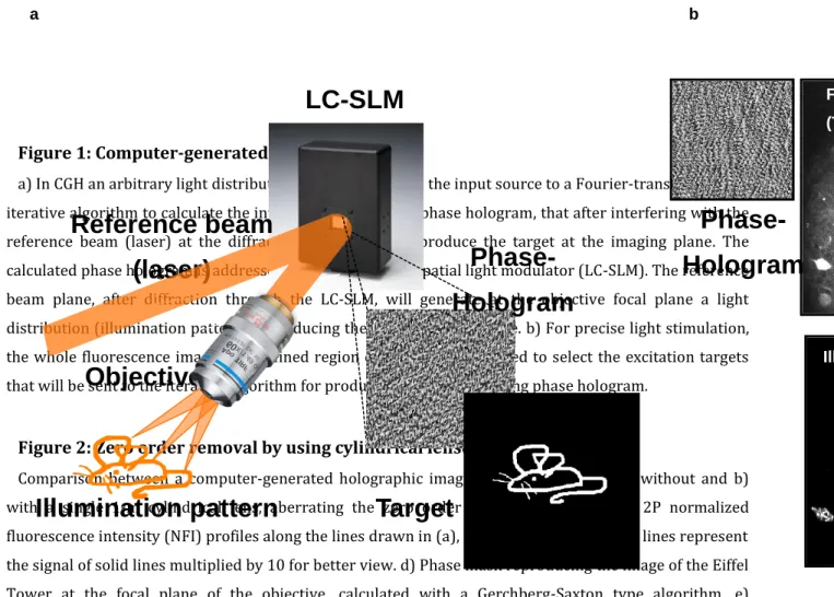
Figure 1: Computer-generated holography
a) In CGH an arbitrary light distribution (target) is used as the input source to a Fourier-transform based iterative algorithm to calculate the interference pattern or phase hologram, that after interfering with the reference beam (laser) at the diffraction plane would reproduce the target at the imaging plane. The calculated phase hologram is addressed to a liquid-crystal spatial light modulator (LC-SLM). The reference beam plane, after diffraction through the LC-SLM, will generate at the objective focal plane a light distribution (illumination pattern) reproducing the original target shape. b) For precise light stimulation, the whole fluorescence image or a defined region of interest can be used to select the excitation targets that will be sent to the iterative algorithm for producing the corresponding phase hologram.
Figure 2: Zero order removal by using cylindrical lenses
Comparison between a computer-generated holographic image of the Eiffel Tower a) without and b) with a single 1-m cylindrical lens, aberrating the zero order in the optical path. c) 2P normalized fluorescence intensity (NFI) profiles along the lines drawn in (a), red, and (b), blue. Dotted lines represent the signal of solid lines multiplied by 10 for better view. d) Phase mask reproducing the image of the Eiffel Tower at the focal plane of the objective, calculated with a Gerchberg-Saxton type algorithm. e) Conjugated cylindrical Fresnel lens hologram added to the one of (d) for aberration compensation. f) Final corrected phase mask addressed to the SLM. Reproduced from Ref. (46).
Figure 3: Diffraction efficiency compensation
a) A graded input image to the iterative algorithm is used to equalize the light distribution across multiple spots (10 μm in diameter) generated on regions of different diffraction efficiency. b) The corresponding light distribution is visualized by illuminating a uniform rhodamine fluorescent layer and by collecting the fluorescence on a CCD camera. Scale bar 30 m. c) Histogram of the normalized average intensity on the spots shown in (b). Intensity is averaged over the area of the spots. Intensity variations among the spots are of the order of 9%.
Figure 4: Axial propagation of holographic beams
Experimental y-z and x-y intensity cross-sections for holographic beams generated to produce at the objective focal plane a) a circular spot, or b) multiple spots of 10-μm diameter. y-z cross-section in (b) is shown along the white dash-dotted line. The yellow circle in both panels approximates the size of a cell
a b Fluorescence (Target)
Phase-Hologram
Laser pattern Illumination patternObjective
LC-SLM
Phase-Hologram
Reference beam
(laser)
Target
Illumination pattern
13
soma. Integrated intensity profiles of y-z cross-sections around the circular spot (a) and in an area covering three spots (dashed yellow) of the multi-spot light configuration (b) are shown on the top of the panels. For comparison, the full width at half maximum of the axial integrated intensity profile of the single 10-μm spot is around 14 μm. Scale bars: 10 μm.
Figure 5: Holographic photostimulation and functional imaging in freely behaving mice
a) Schematic of the holographic fiberscope composed of two illumination paths: one for photoactivation with CGH including a LC-SLM, and a second for fluorescence imaging including a digital micromirror device (DMD). Backward fluorescence was detected on a scientific complementary metal oxide semiconductor (sCMOS) camera. Both paths were coupled to the sample using a fiber bundle attached to a micro-objective (MO). L, Lens; BS, beam splitter; O, microscope objective. b) Left, Calcium signal triggered by photoactivation (blue line; p=50 mW/mm2) with a 5-m diameter holographic spot placed on the somaof a ChR2-expressing cell recorded in a freely behaving mouse co-expressing GCaMP5-G and ChR2 in cerebellar molecular layer interneurons (MLIs). Right, Structure illumination image recorded in a freely behaving mouse and showing MLI somata and a portion of a dendrite (insert). Scale bar: 10 μm. c) Top, The same photoactivation protocol as in (a) was repeated every 30 s for 15 min (photostimulation power, 50 mW/mm2; imaging power, 0.28 mW/mm2). Bottom, Expansion of the top trace showing that
spontaneous activity frequently occurs between evoked transients. Adapted from Ref. (57).
Figure 6: Computer-generated holography and temporal focusing
a) Schematic representation of an experimental setup combining CGH with TF. G: grating, L1 and L2: lenses, BFP: Back focal plane, FFP: Front focal plane. b-c) Experimental y-z and x-y intensity cross-sections for temporally focused holographic beams generated to produce at the objective focal plane a circular spot (b), or multiple spots of 10-μm diameter (c). y-z cross-section in (c) is shown along the white dash-dotted line. Yellow circles approximate the size of a cell soma. Integrated intensity profiles of y-z cross-sections around the circular spot (b) and in an area covering three spots (dashed yellow) of the multispot light configuration (c) are shown on the top of the panels. For comparison, the full width at half maximum of the axial integrated intensity profile of the single 10-μm spot is around 9 μm. The axial confinement thanks to temporal focusing is well preserved, even when multiple spots are projected close together. Scale bars: 10 μm.
Figure 7: Two-photon holographic photostimulation of ReaChR-expressing cells in vivo
The opsin ReaChR was expressed in neurons at layer 2/3 of mouse visual cortex via injection of the viral vector rAAV1-Ef1α-ReaChR-P2A-tdTomato. Positive neurons expressing ReaChR (fluorescent cells in the 2P fluorescence image of the left panel) in isoflurane-anesthetized mouse were photostimulated with a 12-μm diameter excitation spot and 5-ms illumination duration at 0.15 mW/μm2 and λ1030 nm (redshaded area in the right panel). Action potentials were induced by holographic excitation of one positive cell soma (spot 1), whose membrane potential was measured using 2P-guided whole-cell recording (trace 1). Sub-threshold or supra-threshold activation was induced in the patched cell (trace 2-8) upon
14
holographic excitation of spots targeting around its soma (respective radial distance from spot 1 for spots 2-8: 12 µm, 12 µm, 24 µm, 12 µm, 67.6 µm, 40.4 µm, 35 µm), caused by exciting opsin-channels distributed into axon, proximal and distal dendrites of the patched neuron. Scale bar: 40 μm.
Figure 8: ChR2 photocurrent and photocycle
a) Typical photocurrent trace of a CHO cell expressing ChR2 under visible light illumination (1P excitation) for 100 ms. b) Left, schematic of the three-state model where C represents the closed/ground state, O the open state and D the closed/desensitized state. Right, schematic of the four-state model with two closed, C1 and C2, and two open states, O1 and O2. For a detailed description of the model see Ref.
(65).
Figure 9: Temporal resolution and spiking rate
a) Light-elicited single-spike by 2P holographic illumination (spot diameter: 15 m; λ=1030 nm) with short light illumination pulses (t=2 ms) of Chronos (P=0.09 mW/μm2), CoChR (P=0.1 mW/μm2; V.
Zampini, unpublished data) and ReaChR (P=0.07 mW/μm2) expressing interneurons from layer 2/3 of the
mouse visual cortex. b) Light-driven firing fidelity in opsin-positive interneurons by illuminating with a train of 10 light pulses, Chronos (t=2 ms; f=100 Hz; P=0.12 mW/μm2), CoChR (t=3 ms; f=100 Hz; P=0.1
mW/μm2) and ReaChR (t=10ms; f=40 Hz; P=0.04 mW/μm2). The first 4 pulses are zoomed in, in the insets.
Chronos data are adapted from Ref. (29) and ReaChR data are adapted from Ref. (28).
Figure 10: Temporal focusing and penetration depth
a) 2P fluorescence x–y cross-sections of GPC-generated excitation patterns mimicking a neuron with small processes (top) and a 15-μm-diameter CGH spot (bottom) after propagation through 550 μm of acute coronal cortical brain slices without (middle panel) and with (right panel) temporal focusing (λ=950 nm). Non-temporally focused beams are transformed to speckled patterns after traveling through the tissue. b) 2P fluorescence x–y cross-sections of a 20-μm-diameter CGH spot after propagation through the whole brain of a zebrafish larva (~500 μm thick) without (middle panel) and with (right panel) temporal focusing (λ=920 nm). Left panels in all cases are obtained from unscattered beams. Scale bars: 10 μm. Adapted from Refs. (27, 42, 67).
Figure 11: Temporal focusing in the temporal domain
The propagation of a large beam (a holographic spot in this case) diffracted by the grating produces an ultrafast line scanning of the sample. Scattering events off the scanning line at a single moment in time cannot interfere with the ballistic photons in the line. Adapted from Ref. (27).
Figure 12: Multi-plane generation of spatiotemporal focused holographic patterns
a) Schematic of the experimental setup for 3D-CGH-TF. BE: Beam expander, G: diffraction grating, L1, L2, L3, L4: Lenses, OBJ1: Microscope objective. b) Left panel, top, tiled phase profiles addressed to SLM1 for encoding the words ‘neuro’ (plane A) and ‘photonics’ (plane B). Bottom, Fresnel lens-phase profiles15
addressed to SLM2 to axially displace each holographic pattern generated by SLM1 on separated planes at +20 μm (plane A) and -20 μm (plane B). Middle panel, x–y 2P fluorescence intensity cross-sections at planes A and B generated by phase-holograms in the left. Right panel, orthogonal maximum 2P intensity projection along x (top) and y (bottom). c) Axial diffraction efficiency curve, where the intensity of each holographic spot projected at each axial plane is normalized to the one of a spot projected at the center of the nominal focal plane. Experimental data (red points) represent the average of four realizations and follow a Lorentzian distribution (red dashed line) with 0 m. Weighting the axially displaced holographic spot intensity according to the calculated diffraction efficiency enables intensity equalization between holographic patterns in separated axial positions (blue points and dashed line represent the corrected intensity ratio and fitting, respectively). Vertical error bars show the standard deviation for the different realizations. d) Input patterns to the Gerchberg-Saxton algorithm used to calculate the holograms that generate the holographic patterns shown in (b): low-diffraction efficiency regions appear brighter over those closer to the center of the excitation field. To improve the observation of differences between conditions, the amplitude scale of the images was chosen from 0. to 1.5. Adapted from Ref. (42).
Table 1: Kinetics parameters for different opsins
Chronos CoChR ReaChR
on (ms) 0.73 2.4 8
inact (ms) 9.3 200 443
off (ms) 4.2 31 94
Chronos, CoChR and ReaChR were expressed in Chinese Hamster Ovary (CHO) cells following the protocol described in Ref. (28, 29). Electrophysiological data, were recorded 24 – 60 hours after transfection using 2P (λ=950 nm, pulse duration 4s for ReaChR and CoChR and 1s for Chronos; three trials at 1-minute intervals holographic illumination at variable power (from 0.05 mW/µm2 to 1.1 mW/µm2). The current
curves at saturation (defined as the power at which the peak current reaches 90 % of its maximum) where fitted using a mono-exponetial decay for the three transitions: activation, inactivation and deactivation. The corresponding decay times, on (ms), off (ms), inact (ms), are reported in the table and
correspond to power close to saturation (0.86 mW/µm2, 0.54 mW/µm2 and 0.28 mW/µm2 for Chronos,
16
5. References
1. Boyden ES, Zhang F, Bamberg E, et al (2005) Millisecond-timescale, genetically targeted optical control of neural activity. Nat Neurosci 8:1263–1268.
2. Nagel G, Brauner M, Liewald JF, et al (2005) Light activation of Channelrhodopsin-2 in excitable cells of caenorhabditis elegans triggers rapid behavioral responses. Curr Biol 15:2279–2284. doi: 10.1016/j.cub.2005.11.032
3. Zhang F, Wang LP, Brauner M, et al (2007) Multimodal fast optical interrogation of neural circuitry. Nature 446:633–639.
4. Adamantidis AR, Zhang F, Aravanis AM, et al (2007) Neural substrates of awakening probed with optogenetic control of hypocretin neurons. Nature 450:420–4. doi: 10.1038/nature06310
5. Gradinaru V, Thompson KR, Zhang F, et al (2007) Targeting and readout strategies for fast optical neural control in vitro and in vivo. J Neurosci 27:14231–14238.
6. Aravanis AM, Wang LP, Zhang F, et al (2007) An optical neural interface: in vivo control of rodent motor cortex with integrated fiberoptic and optogenetic technology. J Neural Eng 4:S143–S156. 7. Huber D, Petreanu L, Ghitani N, et al (2008) Sparse optical microstimulation in barrel cortex drives
learned behaviour in freely moving mice. Nature 451:61–64.
8. Anikeeva P, Andalman AS, Witten I, et al (2012) Optetrode: a multichannel readout for optogenetic control in freely moving mice. Nat Neurosci 15:163–70. doi: 10.1038/nn.2992
9. Weible AP, Piscopo DM, Rothbart MK, et al (2017) Rhythmic brain stimulation reduces anxiety-related behavior in a mouse model based on meditation training. Proc Natl Acad Sci. doi: 10.1073/pnas.1700756114
10. Makinson CD, Tanaka BS, Sorokin JM, et al (2017) Regulation of Thalamic and Cortical Network Synchrony by Scn8a. Neuron 93:1–15. doi: 10.1016/j.neuron.2017.01.031
11. Petreanu L, Huber D, Sobczyk A, Svoboda K (2007) Channelrhodopsin-2-assisted circuit mapping of long-range callosal projections. Nat Neurosci 10:663–668. doi: nn1891 [pii] 10.1038/nn1891 12. Petreanu L, Mao T, Sternson SM, Svoboda K (2009) The subcellular organization of neocortical
excitatory connections. Nature 457:1142–5. doi: 10.1038/nature07709
13. Tovote P, Esposito MS, Botta P, et al (2016) Midbrain circuits for defensive behaviour. Nature 534:206–212. doi: 10.1038/nature17996
14. Joshi A, Kalappa BI, Anderson CT, Tzounopoulos T (2016) Cell-Specific Cholinergic Modulation of Excitability of Layer 5B Principal Neurons in Mouse Auditory Cortex. J Neurosci 36:8487–99. doi: 10.1523/JNEUROSCI.0780-16.2016
15. Morgenstern NA, Bourg J, Petreanu L (2016) Multilaminar networks of cortical neurons integrate common inputs from sensory thalamus. Nat Neurosci 19:1034–40. doi: 10.1038/nn.4339
16. Lee S-H, Kwan AC, Zhang S, et al (2012) Activation of specific interneurons improves V1 feature selectivity and visual perception. Nature 488:379–83. doi: 10.1038/nature11312
17. Adesnik H, Bruns W, Taniguchi H, et al (2012) A neural circuit for spatial summation in visual cortex. Nature 490:226–31. doi: 10.1038/nature11526
17
Linearly Transform Cortical Responses to Visual Stimuli. Neuron 73:159–170. doi: 10.1016/j.neuron.2011.12.013
19. Klapoetke NC, Murata Y, Kim SS, et al (2014) Independent optical excitation of distinct neural populations. Nat Methods 11:338–346. doi: 10.1038/nmeth.2836
20. Denk W, Strickler JH, Webb WW (1990) Two-photon laser scanning fluorescence microscopy. Science (80- ) 248:73–76.
21. Feldbauer K, Zimmermann D, Pintschovius V, et al (2009) Channelrhodopsin-2 is a leaky proton pump. Proc Natl Acad Sci U S A 106:12317–12322.
22. Rickgauer JP, Tank DW (2009) Two-photon excitation of channelrhodopsin-2 at saturation. Proc Natl Acad Sci U S A 106:15025–15030. doi: 10.1073/pnas.0907084106
23. Andrasfalvy BK, Zemelman B V, Tang J, Vaziri A (2010) Two-photon single-cell optogenetic control of neuronal activity by sculpted light. Proc Natl Acad Sci U S A 107:11981–11986.
24. Prakash R, Yizhar O, Grewe B, et al (2012) Two-photon optogenetic toolbox for fast inhibition, excitation and bistable modulation. Nat Methods 9:1171–9. doi: 10.1038/nmeth.2215
25. Packer AM, Peterka DS, Hirtz JJ, et al (2012) Two-photon optogenetics of dendritic spines and neural circuits. Nat Methods 9:1171–1179. doi: 10.1038/nmeth.2249
26. Rickgauer JP, Deisseroth K, Tank DW (2014) Simultaneous cellular-resolution optical perturbation and imaging of place cell firing fields. Nat Neurosci 17:1816–1824. doi: 10.1038/nn.3866
27. Bègue A, Papagiakoumou E, Leshem B, et al (2013) Two-photon excitation in scattering media by spatiotemporally shaped beams and their application in optogenetic stimulation. Biomed Opt Express 4:2869–2879.
28. Chaigneau E, Ronzitti E, Gajowa AM, et al (2016) Two-photon holographic stimulation of ReaChR. Front Cell Neurosci 10:234.
29. Ronzitti E, Conti R, Papagiakoumou E, et al (2016) Sub-millisecond optogenetic control of neuronal firing with two-photon holographic photoactivation of Chronos. bioRxiv. doi: org/10.1101/062182 30. dal Maschio M, Donovan JC, Helmbrecht TO, Baier H (2017) Linking Neurons to Network Function and Behavior by Two-Photon Holographic Optogenetics and Volumetric Imaging. Neuron 94:774– 789.e5. doi: 10.1016/j.neuron.2017.04.034
31. Papagiakoumou E, Anselmi F, Bègue A, et al (2010) Scanless two-photon excitation of channelrhodopsin-2. Nat Methods 7:848–854. doi: 10.1038/nmeth.1505
32. Oron D, Papagiakoumou E, Anselmi F, Emiliani V (2012) Two-photon optogenetics. Prog Brain Res 196:119–43. doi: 10.1016/B978-0-444-59426-6.00007-0
33. Vaziri A, Emiliani V (2012) Reshaping the optical dimension in optogenetics. Curr Opin Neurobiol 22:128–137. doi: 10.1016/j.conb.2011.11.011
34. Bovetti S, Fellin T (2015) Optical dissection of brain circuits with patterned illumination through the phase modulation of light. J Neurosci Methods 241:66–77. doi: 10.1016/j.jneumeth.2014.12.002
35. Packer AM, Roska B, Häusser M (2013) Targeting neurons and photons for optogenetics. Nat Neurosci 16:805–815. doi: 10.1038/nn.3427
18 175.
37. Gerchberg RW, Saxton WO (1972) A pratical algorithm for the determination of the phase from image and diffraction pictures. Optik (Stuttg) 35:237–246.
38. Lutz C, Otis TS, DeSars V, et al (2008) Holographic photolysis of caged neurotransmitters. Nat Methods 5:821–827. doi: 10.1038/nmeth.1241
39. Papagiakoumou E (2013) Optical developments for optogenetics. Biol Cell 105:443–464. doi: 10.1111/boc.201200087
40. Golan L, Reutsky I, Farah N, Shoham S (2009) Design and characteristics of holographic neural photo-stimulation systems. J Neural Eng 6:66004.
41. Yang S, Papagiakoumou E, Guillon M, et al (2011) Three-dimensional holographic photostimulation of the dendritic arbor. J Neural Eng 8:46002. doi: S1741-2560(11)87640-8 [pii] 10.1088/1741-2560/8/4/046002
42. Hernandez O, Papagiakoumou E, Tanesee D, et al (2016) Three-dimensional spatiotemporal focusing of holographic patterns. Nat Commun 7:11928. doi: 10.1038/ncomms11928
43. Ronzitti E, Guillon M, de Sars V, Emiliani V (2012) LCoS nematic SLM characterization and modeling for diffraction efficiency optimization, zero and ghost orders suppression. Opt Express 20:17843–17855.
44. Polin M, Ladavac K, Lee S-H, et al (2005) Optimized holographic optical traps. Opt Express 13:5831–5845.
45. Zahid M, Velez-Fort M, Papagiakoumou E, et al (2010) Holographic photolysis for multiple cell stimulation in mouse hippocampal slices. PLoS One 5:e9431.
46. Hernandez O, Guillon M, Papagiakoumou E, Emiliani V (2014) Zero-order suppression for two-photon holographic excitation. Opt Lett 39:5953–5956.
47. Conti R, Assayag O, De Sars V, et al (2016) Computer generated holography with intensity-graded patterns. Front Cell Neurosci 10:236.
48. Shemesh OA, Tanese D, Zampini V, et al Single cell optogenetics via combined optical and molecular focusing. Under Rev.
49. Papagiakoumou E, de Sars V, Oron D, Emiliani V (2008) Patterned two-photon illumination by spatiotemporal shaping of ultrashort pulses. Opt Express 16:22039–22047.
50. Golan L, Shoham S (2009) Speckle elimination using shift-averaging in high-rate holographic projection. Opt Express 17:1330–1339. doi: 176064 [pii]
51. Guillon M, Forget BC, Foust AJ, et al (2017) Vortex-free phase profiles for uniform patterning with computer-generated holography. Opt Express 25:12640. doi: 10.1364/OE.25.012640
52. Glückstad J (1996) Phase contrast image synthesis. Opt Commun 130:225–230.
53. Bañas A, Glückstad J (2017) Holo-GPC: Holographic Generalized Phase Contrast. Opt Commun 392:190–195. doi: 10.1016/j.optcom.2017.01.036
54. Schmitz CHJ, Spatz JP, Curtis JE (2005) High-precision steering of multiple holographic optical traps. Opt Express 13:8678–8685.
55. Engström D, Bengtsson J, Eriksson E, Goksör M (2008) Improved beam steering accuracy of a single beam with a 1D phase-only spatial light modulator. Opt Express 16:18275–18287. doi:
19 10.1364/OE.16.018275
56. Hernandez Cubero OR (2016) Advanced optical methods for fast and three-dimensional control of neural activity. Paris Descartes University
57. Szabo V, Ventalon C, De Sars V, et al (2014) Spatially Selective Holographic Photoactivation and Functional Fluorescence Imaging in Freely Behaving Mice with a Fiberscope. Neuron 84:1157– 1169. doi: 10.1016/j.neuron.2014.11.005
58. Oron D, Tal E, Silberberg Y (2005) Scanningless depth-resolved microscopy. Opt Express 13:1468– 1476.
59. Zhu G, van Howe J, Durst M, et al (2005) Simultaneous spatial and temporal focusing of femtosecond pulses. Opt Express 13:2153–2159. doi: 83023 [pii]
60. Baker CA, Elyada YM, Parra-Martin A, Bolton M (2016) Cellular resolution circuit mapping in mouse brain with temporal-focused excitation of soma-targeted channelrhodopsin. eLife 5:1–15. doi: 10.7554/eLife.14193
61. Nagel G, Szellas T, Huhn W, et al (2003) Channelrhodopsin-2, a directly light-gated cation-selective membrane channel. Proc Natl Acad Sci U S A 100:13940–13945.
62. Williams JC, Xu J, Lu Z, et al (2013) Computational Optogenetics: Empirically-Derived Voltage- and Light-Sensitive Channelrhodopsin-2 Model. PLoS Comput Biol 9:e1003220. doi: 10.1371/journal.pcbi.1003220
63. Hegemann P, Ehlenbeck S, Gradmann D (2005) Multiple photocycles of channelrhodopsin. Biophys J 89:3911–8. doi: 10.1529/biophysj.105.069716
64. Nikolic K, Degenaar P, Toumazou C (2006) Modeling and engineering aspects of ChannelRhodopsin2 system for neural photostimulation. In: Annu. Int. Conf. IEEE Eng. Med. Biol. - Proc. pp 1626–1629
65. Nikolic K, Grossman N, Grubb MS, et al (2009) Photocycles of Channelrhodopsin-2. Photochem Photobiol 85:400–411. doi: 10.1111/j.1751-1097.2008.00460.x
66. Lin JY, Knutsen PM, Muller A, et al (2013) ReaChR: a red-shifted variant of channelrhodopsin enables deep transcranial optogenetic excitation. Nat Neurosci 16:1499–1508. doi: 10.1038/nn.3502
67. Papagiakoumou E, Bègue A, Leshem B, et al (2013) Functional patterned multiphoton excitation deep inside scattering tissue. Nat Photonics 7:274–278.
68. Booth MJ, Débarre D, Jesacher A (2012) Adaptive Optics for Biomedical Microscopy. Opt Photonics News 23:22. doi: 10.1364/OPN.23.1.000022
69. Leach J, Sinclair G, Jordan P, et al (2004) 3D manipulation of particles into crystal structures using holographic optical tweezers. Opt Express 12:220.
70. Anselmi F, Ventalon C, Bègue A, et al (2011) Three-dimensional imaging and photostimulation by remote-focusing and holographic light patterning. Proc Natl Acad Sci U S A 108:19504–19509. doi: 10.1073/pnas.1109111108
71. Daria VR, Stricker C, Bowman R, et al (2009) Arbitrary multisite two-photon excitation in four dimensions. Appl Phys Lett 95:93701.
20
of CA1 pyramidal neurons. Front Cell Neurosci 8:127. doi: 10.3389/fncel.2014.00127
73. Packer AM, Russell LE, Dalgleish HWP, Häusser M (2014) Simultaneous all-optical manipulation and recording of neural circuit activity with cellular resolution in vivo. Nat Methods 12:140–146. doi: 10.1038/nmeth.3217
74. Haist T, Schönleber M, Tiziani H. (1997) Computer-generated holograms from 3D-objects written on twisted-nematic liquid crystal displays. Opt Commun 140:299–308. doi: 10.1016/S0030-4018(97)00192-2
75. Zernike F (1942) Phase contrast, a new method for the microscopic observation of transparent objects. Physica 9:686–698. doi: 10.1016/S0031-8914(42)80035-X
76. Glückstad J, Mogensen PC (2001) Optimal phase contrast in common-path interferometry. Appl Opt 40:268–282.