Chaotic mixing by rod-stirring devices in open and closed flows

HAL Id: tel-00204109

https://tel.archives-ouvertes.fr/tel-00204109

HAL is a multi-disciplinary open access archive for the deposit and dissemination of sci-entific research documents, whether they are pub-lished or not. The documents may come from teaching and research institutions in France or abroad, or from public or private research centers.

L’archive ouverte pluridisciplinaire HAL, est destinée au dépôt et à la diffusion de documents scientifiques de niveau recherche, publiés ou non, émanant des établissements d’enseignement et de recherche français ou étrangers, des laboratoires publics ou privés.

closed flows

Emmanuelle Gouillart

To cite this version:

Emmanuelle Gouillart. Chaotic mixing by rod-stirring devices in open and closed flows. Fluid Dy-namics [physics.flu-dyn]. Université Pierre et Marie Curie - Paris VI, 2007. English. �tel-00204109�

T

H`

ESE de

D

OCTORAT de l’

U

NIVERSIT´

E

P

ARIS 6

-PIERRE ET MARIE CURIE

Sp´ecialit´e : Physique

pr´esent´ee par

Emmanuelle Gouillart

pour obtenir le grade de

docteur de l’Universit´e Paris 6 - Pierre et Marie Curie Ecole Doctorale ED 389 :

La Physique de la particule au solide, mod`eles et exp´eriences

Etude de l’advection chaotique dans des m´

elangeurs `

a

tiges, en ´

ecoulements ouverts et ferm´

es

Directeur de recherche : Olivier Dauchot Soutenue le 25 octobre 2007

devant le jury compos´e de :

M. Armand Ajdari . . . Examinateur M. Philippe Carri`ere . . . Rapporteur

M. Olivier Dauchot . . . Directeur de th`ese M. Jean-Pierre Hulin . . . Rapporteur

M. Franck Pigeonneau . . . Membre invit´e M. St´ephane Roux . . . Examinateur M. Jean-Luc Thiffeault . . . Directeur de th`ese M. St´ephane Zaleski . . . Pr´esident

Service de Physique de l’Etat Condens´e, CEA Saclay Department of Mathematics, Imperial College London

R´

esum´

e

Nous avons ´etudi´e le m´elange de fluides visqueux dans des ´ecoulements 2-D ouverts et ferm´es o`u des agitateurs cr´eent de l’advection chaotique, i.e. des trajectoires lagrangiennes complexes. Notre ´etude, exp´erimentale, num´erique et th´eorique, s’appuie sur deux types d’exp´eriences de m´elange chaotique, en domaine ferm´e et dans un canal ouvert. En syst`eme ferm´e, nous avons d’abord propos´e une caract´erisation topologique du m´elange reposant sur l’enchevˆetrement des trajectoires de points p´eriodiques – les “tiges fantˆomes”. D’autre part, l’´etude exp´erimentale du champ de concen-tration d’un colorant nous a permis de d´ecrire le rˆole des murs du domaine o`u se fait le m´elange, pour les ´ecoulements ferm´es comme ouverts. En ferm´e, la nature chaotique ou r´eguli`ere des trajectoires initialis´ees pr`es des bords d´etermine l’´evolution du champ de concentration, mˆeme loin des bords. Nous avons ainsi observ´e une dynamique lente (alg´ebrique) de l’homog´en´ei-sation quand la r´egion chaotique s’´etend jusqu’`a des murs non-glissants. En ouvert, nous avons d´ecrit l’´evolution du champ de concentration dans, et en aval de la r´egion de m´elange, r´esultant de l’injection d’un blob de colorant. Nous avons d´ecrit les ´el´ements mal m´elang´es qui s’´echappent aux temps courts, et l’apparition d’un motif permanent (auto-similaire) aux temps longs, d´etermin´e par les orbites p´eriodiques de la r´egion de m´elange. Des modifications de ce sc´enario apparaissent quand la r´egion de m´elange va jusqu’aux murs. Enfin, une mod´elisation `a base de transformation du bou-langer g´en´eralis´ee nous a permis de comprendre l’essentiel des m´ecanismes rencontr´es.

Mots-cl´es : m´elange chaotique, m´elangeur industriel, fluides visqueux, strange eigenmode, syst`emes ouverts, selle chaotique, transformation du boulanger, m´elange topologique, orbites p´eriodiques.

Abstract

We have studied the mixing of viscous fluids in 2-D closed and open flows, where stirring rods create chaotic advection, i.e. complex Lagrangian tra-jectories. Our study, experimental, numerical and theoretical, is based on two types of chaotic mixing experiments, in a closed vat and in an open channel. For closed flows, we have first proposed a topological descrip-tion of mixing by the entanglement of periodic orbits that we called ”ghost rods”. The experimental study of the concentration field of a dye has then revealed the role of the walls of the domain where mixing takes place, in closed and open flows as well. For closed flows, the chaotic or regular nature of trajectories initialized close to the wall determines the evolution of the concentration field, even far from the walls. In particular, we have observed slow (algebraic) dynamics of homogenization when the chaotic region ex-tends to no-slip walls. In open flows, we have reported on the evolution of the concentration field in the mixing and downstream regions, resulting from the injection of a dye blob. We have described the poorly mixed ele-ments that escape quickly, as well as the asymptotic onset of a permanent (self-similar) pattern determined by the periodic orbits inside the mixing region. Finally, various models derived from the baker’s map have allowed us to understand most observed mechanisms.

Keywords : chaotic mixing, industrial mixers, viscous fluids, strange eigenmode, open flows, chaotic saddle, baker’s map, topological mixing, periodic orbits.

Remerciements

Les travaux pr´esent´es dans ce manuscrit ont ´et´e r´ealis´es d’abord au d´epartement de math´ematiques appliqu´ees de l’Imperial College `a Londres, puis au Service de Physique de l’Etat Condens´e du CEA Saclay. Cette th`ese CIFRE a ´et´e financ´ee par l’entreprise Saint-Gobain Recherche, que je souhaite remercier pour m’avoir donn´e cette belle opportunit´e d’ˆetre form´ee `a la recherche, et ce dans d’excellentes conditions.

Je souhaiterais tout d’abord exprimer ma profonde gratitude `a mes deux directeurs de th`ese, Olivier Dauchot et Luc Thiffeault. Olivier et Jean-Luc ont ´et´e pour moi des encadrants exceptionnels, mais aussi des amis. Ils ont su me faire profiter de leur exp´erience et m’apprendre la recherche, tout en me laissant toujours la libert´e dont j’avais besoin. Ils sont donc pour beaucoup dans le plaisir et l’´epanouissement que j’ai pu trouver dans cette th`ese. Jean-Luc a fait preuve de beaucoup de p´edagogie pour me transmettre sa vision tr`es compl`ete du m´elange chaotique. Son exp´erience de la programmation m’a ´egalement beaucoup appris, et nos nombreuses conversations « geek » ont ´et´e un plaisir. Si l’anglais de ce manuscrit est `a peu pr`es lisible, c’est en grande partie grˆace `a lui, qui a su gentiment ignorer mes sarcasmes sur l’accent qu´eb´ecois pour plutˆot apprendre `a sa th´esarde frenchie `a parler et ´ecrire un peu mieux anglais. Olivier a relev´e le d´efi d’apprendre `a faire des manips `a une th´esarde – alors – th´eoricienne, venue tout droit de la topologie et des tresses. J’ai aussi beaucoup b´en´efici´e de sa grande culture scientifique, et de son exp´erience dans le traitement et l’analyse des donn´ees. L’ambiance d´etendue et l´eg`erement euphorique qu’il transporte avec lui a largement contribu´e au plaisir que j’ai eu `a travailler sous sa direction.

Je voudrais ´egalement remercier tr`es chaleureusement St´ephane Roux. Ma th`ese doit beaucoup `a ses interventions lumineuses ; je lui suis notam-ment redevable des « petits mod`eles » d´eriv´es de l’application du boulanger, et je le remercie pour ses patientes tentatives pour m’insuffler un peu de sa rigueur et de sa logique impressionnantes. Cette collaboration passionnante a ´egalement ´et´e tr`es agr´eable grˆace `a sa gentillesse et sa disponibilit´e.

J’ai aussi beaucoup b´en´efici´e de l’expertise et de l’encadrement des cher-cheurs du GIT (l’in´enarrable Groupe Instabilit´es et Turbulence, du Service de Physique de l’Etat Condens´e du CEA Saclay). Merci `a B´ereng`ere Du-brulle, dont j’ai partag´e le bureau pendant mon s´ejour au CEA : sa verve romanesque contribue grandement `a l’ambiance du groupe, et si je n’ai su exploiter qu’une partie de sa myriade d’id´ees, nos discussions ont ´et´e tr`es enrichissantes. Je remercie aussi vivement Fran¸cois Daviaud pour m’avoir accueillie dans son groupe (lourde charge que d’ˆetre responsable du GIT !) mais aussi pour m’avoir fait profiter de son savoir-faire d’exp´erimentateur et de ses connaissances en physique non-lin´eaire. Son aide lors des premiers mois de mon s´ejour au CEA a ´et´e pr´ecieuse, et je lui en suis tr`es reconnais-sante. Merci ´egalement `a Arnaud Chiffaudel pour ses coups de pouce exp´e-rimentaux, son esprit critique et son enthousiasme scientifique. Merci `a Eric Vincent pour m’avoir accueillie au Service de Physique de l’Etat Condens´e, s’ˆetre int´eress´e `a mon travail et avoir sign´e sans sourciller les commandes de centaines de litres de Canadou, et de divers colorants exotiques. Je vou-drais ´egalement remercier nos incomparables techniciens C´ecile Gasquet et Vincent Padilla, grˆace `a qui monter et faire fonctionner une manip devient une tˆache agr´eable en plus d’ˆetre instructive. Merci `a Vincent le m´ecanicien po`ete pour la qualit´e de son travail et pour son amiti´e. Merci `a C´ecile pour son efficacit´e infatigable et pour ne pas avoir h´esit´e `a mettre ses mains dans le Canadou avec moi lors des phases les plus ingrates des manips.

A Imperial College, j’ai eu beaucoup de plaisir `a travailler avec Matt Finn : derri`ere son flegme si britannique et sa modestie, Matt cache une rigueur et une cr´eativit´e admirables. Nombre de r´esultats pr´esent´es dans cette th`ese ont ´et´e obtenus `a partir des codes d’advection lagrangienne con¸cus et d´evelopp´es par lui.

A Saint-Gobain Recherche, au service Elaboration des Verres puis `a l’Unit´e mixte Saint-Gobain/CNRS, Franck Pigeonneau a ´et´e un collabora-teur pr´ecieux : j’ai pu b´en´eficier `a de nombreuses reprises de ses connais-sances en hydrodynamique, et les r´esultats de ses simulations num´eriques sont `a la base de certaines orientations dans mon travail. Je remercie ´egale-ment Laurent Pierrot, chef du groupe Physique de la Fusion, pour l’int´erˆet qu’il a port´e `a mon travail tout au long de ma th`ese, et pour ses nom-breuses questions, toujours judicieuses. Jacques-Olivier Moussafir nous a procur´e quelques excursions m´emorables dans le monde merveilleux de la topologie o`u il se prom`ene avec un naturel d´econcertant, et un grand sou-rire. Je le remercie ´egalement pour son code de calcul d’entropie topologique des tresses. Jean-Marc Flesselles a identifi´e ce beau sujet qu’est le m´elange chaotique dans les ´ecoulements ouverts, et est `a l’origine de la collaboration entre les diff´erentes ´equipes qui ont encadr´e ma th`ese : je ne saurais assez

9

l’en remercier. Mes remerciements vont ´egalement `a Herv´e Arribart pour avoir s´electionn´e ce projet sur le m´elange parmi les th`eses financ´ees par Saint-Gobain, et pour l’int´erˆet qu’il a port´e `a mon travail.

Philippe Cari`erre et Jean-Pierre Hulin ont accept´e la lourde tˆache d’ˆetre rapporteurs : je les remercie pour la pr´ecision de leur lecture et la pertinence de leurs questions, qui ont certainement am´elior´e ce manuscrit. Je remercie ´egalement Armand Ajdari et St´ephane Zaleski de m’avoir fait le plaisir et l’honneur de participer `a mon jury.

Cette th`ese n’aurait pas ´et´e aussi agr´eable sans l’ambiance tr`es sympa-thique des diff´erentes ´equipes o`u j’ai travaill´e. A Londres, les soir´ees DVD chez Jean-Luc avec sa « dream team », Matt, Khalid Kamhawi, et Lennon O’Naraigh, ou les fins d’apr`es-midi au pub avec le groupe de dynamique des fluides sont autant d’excellents souvenirs. A Saclay, le GIT tout entier est un microcosme extraordinaire, qu’il est difficile de quitter : outre les personnes d´ej`a cit´ees, je remercie ses membres permanents Marco Bonetti, S´ebastien Aumaitre et Patrick M´eninger, mes camarades th´esards Rapha¨el Candelier, Fr´ed´eric L´echenault, Guillaume Marty, Romain Monchaux et Florent Ra-velet, et ses « membres d’´election » Daniel Bonamy et Elisabeth Bouchaud. Je remercie aussi ma stagiaire Natalia Kuncio pour son excellent travail sur le m´elangeur en huit. Apr`es l’effort, le r´econfort : les soir´ees `a l’Olisph`ere, et les bi`eres au « bar des sciences » du sous-sol – qui deviendra vite une institution, j’en suis sˆure – me laissent de tr`es beaux souvenirs. A Saint-Gobain Recherche, l’aventure continue puisque j’ai la chance de rejoindre pendant quelques mois le sympathique groupe Physique de la Fusion, o`u j’ai toujours ´et´e chaleureusement accueillie pendant ma th`ese.

Je souhaiterais ´egalement exprimer ma reconnaissance `a l’ensemble de la communaut´e des d´eveloppeurs de logiciels libres. Il ne m’aurait sans doute pas ´et´e possible d’explorer autant de pistes ou de tester rapidement de nombreuses id´ees plus ou moins farfelues sans la puissance et la souplesse du syst`eme d’exploitation Linux, et la multitude de logiciels scientifiques libres et de grande qualit´e qui existent grˆace `a cette communaut´e.

Merci `a ma famille pour son soutien et son affection. Ma famille et mes amis ont accept´e avec le sourire de ne pas me voir beaucoup pendant ces trois ans, et je les en remercie. Merci `a notre coloc Jonas pour son amiti´e et nos discussions, notamment sur les ondelettes. Merci `a mon cher Ga¨el, dont la pr´esence est la source de tant de joies ; ces ann´ees de th`ese ont ´et´e illumin´ees par son soutien quotidien et l’enthousiasme avec lequel il s’est int´eress´e `a mes travaux.

Contents

Contents 11

1 Introduction 13

1.1 Industrial motivation for studying fluid mixing . . . 13

1.2 Basic mixing mechanisms in viscous fluid flows . . . 16

1.3 Outline of the thesis . . . 29

2 The mixing systems 31 2.1 Selection of the mixing protocols . . . 31

2.2 Experimental set-up . . . 36

2.3 Numerical simulations of Stokes flows . . . 52

2.4 Conclusion . . . 54

3 Dynamical systems structures 57 3.1 Dynamical systems concepts in mixing . . . 57

3.2 A topological characterization of mixing in closed flows . . . 63

3.3 Chaotic saddle: periodic orbits in open flows . . . 87

3.4 Conclusion . . . 99

4 Homogenization in closed flows 101 4.1 Homogenization mechanisms . . . 102

4.2 Mixing in fully hyperbolic systems: the onset of strange eigenmodes . . . 108

4.3 Mixing in bounded domains fully covered by a chaotic region 115 4.4 Case of an elliptic region near the wall . . . 144

4.5 Discussion . . . 149

5 Homogenization in open flows 151 5.1 Introduction – similarities with homogenization in closed flows . . . 152

5.2 Butterfly case . . . 155

5.3 Breaststroke case . . . 173

5.4 Conclusion . . . 183

6 Measures of mixing in open flows 185 6.1 Usual strategies for characterizing mixing . . . 186

6.2 Quantifying mixing in open flows . . . 193

6.3 Conclusion . . . 212

7 Conclusions 215 7.1 Summary of approach . . . 215

7.2 Summary of results . . . 216

7.3 A few take-home messages . . . 220

7.4 Perspectives - outlook on future work . . . 222

Bibliography 223

Chapter 1

Mixing viscous fluids: a

general introduction

The work presented in this thesis is an attempt to describe and classify some generic features of mixing mechanisms leading to homogenization of fluids. We will mostly consider homogenization realized by two-dimensional laminar (non-turbulent) closed and open flows. Despite the apparent variety of industrial mixing processes, we wish to draw here universal characteristics that may help the engineer in designing new mixers and assessing their efficiency.

1.1

Industrial motivation for studying fluid

mixing

Many industrial applications would benefit greatly from further insight into the mixing mechanisms of viscous fluids. Fields as diverse as chemical en-gineering, polymer processing , the pharmaceutical and cosmetics industry, pulp and paper industry, or food processing rely on processes where ini-tially heterogeneous fluids are stirred together to obtain a product with a sufficient degree of “mixedness”, a generic property that might stand for chemical and/or thermal homogeneity, mechanical properties (e.g. stiff-ness) spatial homogeneity, etc., depending on the desired qualities of the final product.

Depending on processes, mixing operations are realized in closed vats or open-flow continuous mixers (see Fig. 1.1). Most devices rely on moving stirrers (e.g. whisks in eggbeater-like devices) and mobile boundaries, or constrained mixer geometries (e.g. food processing screw extruders). There is a vast engineering literature dealing with the extensive study of mixing

(a) (b) (c)

Figure 1.1: Some examples of fluid mixers, from everyday life to industrial applications. (a) Egg beater. (b) Batch planetary mixer used in food processing. (c) Throughflow SMX mixer.

devices; for a review see e.g. the handbook [84]. However, what we aim to do here is in a sense the opposite approach to a handbook: instead of characterizing the difference and uses of a variety of devices, we wish to find general characteristics of fluid mixers.

For the engineer as for the physicist, two main issues arise immediately when considering mixing.

• First, it is of crucial importance to gain sufficient insight into physical mixing mechanisms to predict the rate of mixing that can be achieved by mixers. Common wisdom suggests that “the harder and faster you stir, the more you mix”. Yet, precise knowledge of homogenization is necessary to achieve mixing at lowest cost, or while designing mixing installations. Also, the same mixing device may be used successively in various situations where different mixing qualities are required. A priori knowledge of generic mixing characteristics spares the time and money consuming process of repeated trial and error for tuning pa-rameters such as flow rate, stirrer size and velocity, process duration, etc. Another requirement is to find laws that are valid for different initial conditions.

Consider for example the simple mixer shown in Fig. 1.2. A cylindrical rod stirs repeatedly viscous sugar syrup on a figure-eight path – which is basically how you would stir chocolate with other cake ingredients in a cooking bowl. No chocolate is used here, instead we initially mark a small patch of fluid with ink. The filamentary pattern created by the rod movement evolves with time and progressively fills a large domain (see different stages of this evolution in Fig. 1.2). At each

1.1. INDUSTRIAL MOTIVATION FOR STUDYING FLUID MIXING15

(a) (b)

(c) (d)

Figure 1.2: Homogenization of a viscous flow with a simple stirring device (experiments described later in the thesis). A cylindrical rod stirs viscous sugar syrup by moving periodically on a figure-eight (∞) path. We visualize the mixing of an initial blob of dye after 2 (b), 4 (c) and 8 (d) periods of the stirring protocol. To characterize our mixer, we need to understand “how fast it mixes”, that is how the mixing pattern develops and what is the degree of homogeneity of such a pattern.

instant, this pattern is fully characterized by the dye concentration field C(x, t), which evolves towards homogeneity as time progresses. One of the first tasks is therefore to describe this mixing pattern, e.g. by studying the concentration field statistical properties, in order to give a first answer to the question: How fast does it mix ? As we will see in Chapter 4, the answer is far from obvious.

• On the other hand, if one stirs the fluid with a different protocol than the figure-eight, we expect to see a different dye pattern. Another challenge in mixing processes is therefore to have at hand a collec-tion of criteria for evaluating the mixing quality achieved by various mixers. One could naively conclude that evaluating mixing efficiency amounts to comparing mixed products qualities. Such an approach is in practice not sustainable. For example, an open-flow mixer might be composed of successive stirring parts that have to be compared inde-pendently, regardless of the final product. Also, complete information about the partly mixed state (that is C(x, t)) is not always avail-able, and mixers must be evaluated from partial information, such as pictures of the mixing pattern (Fig. 1.2). Also, nonintrusive mixing measures might be required in situations where one wishes to follow the mixing evolution without disturbing the system.

These two problems are of course intimately linked, and deciding which one to study first is quite a chicken and egg dilemma. The study of mixing mechanisms may reveal features of the partly mixed system – such as the spatial structure of the mixed pattern, or the amplitude of worst hetero-geneities – from which extensive information about the mixedness of the system can be gained. If easily measurable, these quantities will be relevant candidates for characterizing mixing. On the other hand, describing the speed of mixing supposes a proper evaluation of the mixing state achieved at each time.

1.2

Basic mixing mechanisms in viscous

fluid flows

We briefly present here a few common-wisdom elements aiming at answering the first question we suggested: how fast does it mix ? This paragraph was partly inspired by the introductory chapter of Ottino’s reference textbook on mixing [82].

1.2. BASIC MIXING MECHANISMS IN VISCOUS FLUID FLOWS 17

1.2.1

A simple picture

Although we have defined the aim of fluid mixing, that is homogenization, we have not yet characterized how mixing takes place. The successive pic-tures of Fig. 1.2 can help us to draw some building blocks of fluid mixing. Let us consider viscous fluid inside a mixer, initially seeded with some in-homogeneity, e.g. a blob of dye.

• Mobile parts of the device – such as the stirring rod in Fig. 1.2 (a) –, or geometry changes for continuous mixers, create a flow that is spatially heterogeneous. Velocity gradients, that is shears, deform locally fluid elements along preferred directions. The stirring rod in Fig. 1.2 (b) stretches for example the dye blob in its wake.

• Stretching of fluid elements causes the blob frontier to grow and the blob to be dispersed in a larger domain than it occupied at first – although its area remains constant in incompressible flows. This shuf-fling of fluid elements is the first ingredient of mixing: fluid elements initially close do not stay together but are instead dispersed over the fluid domain.

• However, this purely geometric rearrangement does not account for the whole mixing process. The mixing pattern on Fig. 1.2 (d) is not just a zebra-like juxtaposition of black and white fluid elements; in-termediate gray levels are visible instead. This is due to molecular diffusion that blurs material contours and allows initially separated regions to interpenetrate each other. The action of diffusion is more spectacular on thin filaments, as it is then faster for the unmarked fluid particles to contaminate the dye filament to its core through random walking – a process responsible for the fading of black and white contrast. The stirring of fluid elements in thin filaments – a purely kinematics mechanism – facilitates intimate mixing realized by diffusion at the molecular scale. Also note that different gray lev-els along the elongated blob result from different stretching histories experienced by the particles.

One of the requirements for an efficient stirring velocity field is there-fore to create small scales at which diffusion can act within a reasonable timescale. This might seem a challenge for laminar flows: unlike turbulent ones, low-Reynolds-number velocity fields have significant energy only at the integral scale of the flow (such as the scale of the flow domain, or the stirrer’s size). They do not benefit from the short-correlated velocity fluctu-ations – and hence stretching – that act at various scales and lead to efficient

Figure 1.3: Turbulent mixing, experiments by Villermaux and Duplat [125]. In this turbulent flow, small-scale velocity fluctuations create random shears that stretch fluid in random directions and homogenize fluid uniformly across the domain. Note that the dye pattern is very different from the pattern in viscous fluid (Fig. 1.2).

mixing in turbulent flows, as can be observed in Fig. 1.3. On the contrary, we consider from now on smooth large-scale stirring flows with simple time dependence (stationary or time-periodic). Flow Reynolds numbers, defined by Re = U ℓ/ν, where U is a typical flow velocity, ℓ the typical flow scale and ν the fluid kinematical viscosity, will be small, typically Re_{∼ 1 . The} mixing pattern created in very viscous sugar syrup by the rod in Fig. 1.2 is very different from the turbulent one in Fig. 1.3; filaments are nicely packed in parallel structures, and not randomly pointing in rapidly varying directions, as in the turbulent case. One can also note that some parts of the domain are not contaminated by the dye expansion. One of the mech-anisms we wish to describe is how a large-scale flow can create these thin filamentary structures.

1.2. BASIC MIXING MECHANISMS IN VISCOUS FLUID FLOWS 19

1.2.2

Open flows: a transient stretching

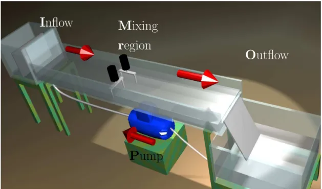
We also aim at understanding and characterizing mixing in open flows. By open-flow mixers, we mean devices where a main flow crosses a mixing region where fluid particles are stretched as in the closed flow case. An example is shown on Fig. 1.4: viscous sugar syrup flows through a long shallow channel; constant flow rate imposes a stationary flow in the far upstream and downstream of the “mixing region”, where two rods stir fluid in an egg-beater-like fashion. Another class of open-flow mixers, that will not be studied here, consists of the space-periodic juxtaposition of successive passive mixing elements such as bends or bas-relief structures along the main flow direction (these mixers are e.g. frequently used in microfluidics).

Mixing in open flows also relies on stretching and diffusion , with a crucial difference: the main flow that forces fluid particles to be carried away downstream. As a blob of inhomogeneity flows from upstream, a fraction is caught by the rods, stretched and folded in a complicated pattern (Fig. 1.4 (b) and (c)) as in closed flows. Note that the filamentary pattern around the rods in Fig. 1.4 (c) has some similarities with the one in Fig. 1.2 (d); the same combination of stretching and diffusion create intermediate grey levels with fading contrast. Nevertheless, contrary to closed flows, some dye particles are never caught inside the mixing region, but escape downstream without having experienced much stretching (the black lobes on top of Fig. 1.4 (b)). Also, because of the main flow that pushes fluid downstream, fluid leaks continuously from the mixing region, resulting in the “flower” pattern with partly mixed lobes shown in Fig. 1.4 (c)). This is due to the main flow: fluid particles that come from upstream must eventually escape downstream. However, fluid particles initially in the same small blob of dye (Fig. 1.4 (c)) can experience very different stretching and mixing history, depending on the time they spend in the mixing region. In closed flows, all particles spend the same time in the mixer; this is not the case in open flows where the chance to be stretched depends strongly on the initial condition. The escape process is irreversible: once a fluid particle leaves the mixing region, it cannot experience much more stretching – of course, diffusion continues to homogenize the filaments, and some additional stretching might be caused by a spatially nonuniform downstream flow, such as a Poiseuille flow, but for the cases we consider, the latter effect is weaker compared to the stretching realized by our rods. Thus, the fate of a fluid particle depends strongly on the particle residence time inside the mixing region. This explains the success of residence time distribution analyses used in the chemical engineering field since Danckwerts [30] to characterize mixing in open flows.

(a) (b)

(c)

Figure 1.4: Mixing in open flows: a transient process. (experiments described later in the thesis) (a) Viscous fluid (sugar syrup) flows in a long shallow channel at a constant flow rate. Two rods stir the passing fluid in an egg-beater-like fashion (the two rods move on intersecting circles in opposite senses). A blob of incoming fluid is marked with dye. (b) A fraction of the blob is caught by the rods inside the mixing region where it is stretched and folded in many filaments. However, other parts of the blob escape from the mixing region barely stretched. These are the thick black structures on top of the snapshot: they are very poorly-mixed and will not get any other chance to experience more mixing. (c) As time goes on, dyed fluid keeps leaking from the mixing region. The longer marked particles stay in the mixing region, the more stretching they experience: escaping lobes in the near downstream region look therefore more and more mixed – in a sense that has yet to be specified.

1.2. BASIC MIXING MECHANISMS IN VISCOUS FLUID FLOWS 21

A necessary condition for good mixing in open flows is therefore to keep fluid particles inside the mixing region as long as possible so that they experience enough stretching. One could naively conclude that the right solution is then to increase the stirrers velocity, or equivalently to decrease the average flow rate, so that a particle spends on average more stirring periods inside the mixing region. However, flowrate directly controls the productivity in continuous open-flow mixing systems and decreasing it too much is usually undesirable. Conversely, the energetic cost of moving the stirrers faster might be prohibitive; fragile polymers might also forbid the use of hight stirring velocities . Besides, this tuning only changes the aver-age residence time of particles inside the mixing region, and typical open-flow mixers create a broad residence-time distribution for fluid particles (cf. Fig. 1.4). Particles that escape faster than the mean residence time, like the thick black lines on Fig. 1.4 (b), are especially problematic. More in-sight into the range of histories of fluid particles in open flows is therefore necessary to characterize mixing.

1.2.3

The framework of chaotic advection: a study

of Lagrangian dynamics

Now that we have introduced that homogenization results from the com-bination of stretching through stirring, and diffusion , we wish to relate quantitatively this process to an evaluation of the evolving mixing state of, say, a blob of dye. A first attempt in this direction may be to write directly the advection-diffusion equation

∂C

∂t + v· ∇C = κ∆C, (1.1) which determines completely the evolution of the dye concentration field C(x, t), given suitable initial conditions. v is the stirring velocity field and κ the diffusion coefficient. However, this partial differential equation cannot be solved analytically in most cases. Only numerical integration of (1.1) can usually solve for C. Spectral methods allow to obtain the concentration field with a very good accuracy, yet other methods that suffer from numerical diffusion must somtimes be used for complicated geometries.

Generally, the Eulerian field v gives little information about the devel-opment of the mixing pattern. As we described in the previous paragraph, a natural description of mixing rather comes from following the stretching of elementary elements, or fluid particles – a Lagrangian description. Fortu-nately, such a description can be made in the rich framework of dynamical

systems, as we will describe throughout this paragraph. Indeed, if we con-sider the motion of a passive fluid element in a given velocity field v, the trajectory of the fluid particle will be given by integrating the equation:

˙x(t) = vparticle(x, t) = vfluid(x, t), (1.2) that is ˙x(t) = u(x, y, z, t) (1.3) ˙y(t) = v(x, y, z, t) (1.4) ˙z(t) = w(x, y, z, t) (1.5) in 3-D flows, or ˙x(t) = u(x, y, t) (1.6) ˙y(t) = v(x, y, t) (1.7) in 2-D flows, on which we will mostly focus throughout this thesis.

The particle therefore evolves in a phase space whose dimension is given by the dimension n of the flow (n = 2 or 3 for physical fluid flows), plus an optional additional degree of freedom if the velocity field is time-dependent. Even for simple regular flows, the components of v are generically nonlinear functions of the coordinates. A three-dimensional phase space is enough for a nonlinear dynamical system to exhibit chaotic trajectories, that is extreme sensitivity to initial conditions (for a general introduction to dy-namical systems, chaos and its applications, see the textbooks [67] and [14], or the more technical monographs [79] and [3].). A famous example is the three-dimensional system proposed by Lorenz to model convection [66] (it is a dissipative system, however). Two-dimensional time-dependent flows or three-dimensional stationary flows can therefore create chaotic trajectories. This situation is most beneficial for mixing, as two fluid particles initially close to each other (e.g. two marked particles inside the initial blob of dye) separate very fast – in fact, exponentially with time as predicted by the Lyapunov exponent of the flow (see Fig. 1.5) – and won’t stay segregated in the same small area. For finite systems, this is only true until the sep-aration is on the order of the system size. Another way to understand the advantages of chaos for mixing is to realize that points on the blob frontier will separate exponentially, hence the frontier will grow exponentially with time. In incompressible flows, mass conservation imposes in return that the size of the blob in the direction transverse to stretching decreases exponen-tially, thus facilitating the action of diffusion as we saw. Unlike many other domains, fluid mixing hence benefits from chaos!

1.2. BASIC MIXING MECHANISMS IN VISCOUS FLUID FLOWS 23

The alert reader may now ask which suitable velocity fields (in Eq. (1.2)) might create such chaotic trajectories. As a general rule of thumb, flows can create chaotic trajectories, or equivalently exponential stretching, if fluid particles experience successively shears in transverse directions. Fig. 1.6 illustrates this condition. Fig. 1.6 (a) shows the mixing of a blob by a vortex-flow realized by Meunier and Villermaux [70]. In this stationary radial-shear flow, fluid particles align with flow streamlines on a spiral and are always stretched along the same direction. No chaotic trajectories can be created by this flow, where adjoining particles separate linearly with time, as in a classical shear flow. On the other hand, we can see on Fig. 1.6 (b) the deformation of a blob by the eight protocol. Because of the figure-eight _{∞ shape, the rod can cross the origin in two transverse directions,} ւ and ց. On Fig. 1.6 (b), the passing rod has first stretched the blob and aligned some part of it along the ւ direction. However, half a period later the rod will stretch the blob, yet in the _{ց direction this time. One} can easily check that such a succession of stretching in different directions causes the distance between two particles to grow exponentially with time – a distinctive feature of chaos. Such mechanisms have been successfully studied of the linked twist map framework [130, 106]

0

t

l

l

(t) = l

e

Figure 1.5: Sensitivity to initial conditions: in a chaotic flow, two neigh-boring particles separate exponentially with time and their distance grows as l(t) = l0eλt during time t. λ is referred to as the stretching coefficient for the

corresponding fluid particles, or finite-time Lyapunov exponent. As a conse-quence, material blobs are exponentially stretched along the separating direc-tion. Note that particles at different locations may experience different finite-time stretching coefficients.

The ability for simple flows to create complicated – chaotic – trajectories was named chaotic advection by Aref in a seminal paper [8]. For the first time, Aref linked the familiar Lagrangian approach in fluids, and the then-recent discovery than dynamical systems could exhibit chaos. In this paper, Aref considered in particular the case of two-dimensional incompressible time-dependent flows, for which the equations of motion have a Hamiltonian form , due to the existence of the stream function Ψ:

˙x(t) = u(x, y, t) =−∂Ψ

∂y (1.8)

˙y(t) = v(x, y, t) = ∂Ψ

∂x. (1.9)

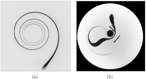
The coordinates x and y are conjugated Hamiltonian variables, and the phase space is also the real physical space (x, y) of the experiment ! This property allows visualization of the beautifully elongated structures of chaos directly in dye spreading experiments as on Fig. 1.2, and explains partly all

(a) (b)

Figure 1.6: Two possible stretching scenarios: simple-shear or chaotic flows. (a) Experiments by Meunier and Villermaux [70]. A vortex creates a radial shear flow that stretches a blob of dye linearly with time along a smooth spiral. No chaotic trajectories can be created by such a protocol, as in a stationary flow, particles trajectories coincide with streamlines. (b) In the figure-eight (_{∞) protocol, the self-crossing trajectory of the rod imposes that particles are} successively stretched along transverse directions. This multiplicative stretching process imposes that neighboring particles separate exponentially with time on chaotic trajectories.

1.2. BASIC MIXING MECHANISMS IN VISCOUS FLUID FLOWS 25

the enthusiasm generated by chaotic advection since 20 years (for a review see [82]).

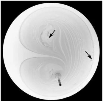
However, a generic phase space is rarely entirely chaotic; usually, chaotic regions coexist with regular regions where stretching is not exponential, but at most algebraic with time. Fig. 1.7 (b) illustrates this coexistence. We have computed a so-called Poincar´e section for two variants of our now-familiar figure-eight stirring-rod protocol. A Poincar´e section consists in representing the regions that are visited by trajectories of single fluid par-ticles, stroboscoped at each period of the stirring protocol. For obtaining Fig. 1.7 (b), we have integrated numerically the trajectory of a few initial conditions during a large number of periods of the protocol and we have represented the stroboscoped position of the particles at each period. The integration was realized using the Stokes flow described in [40] for the rod motion. For the protocol represented on Fig. 1.7 (a), a single particle tra-jectory fills the entire domain: we conclude that almost all trajectories are chaotic (there could be tiny islands not visible on the section). However, for a protocol with a smaller rod, Fig. 1.7 (b) reveals the presence of two small islands where the stroboscoped positions of particles (red points) are confined to elliptical paths . These two islands, and the large chaotic sea surrounding them, are an example of mixed phase space. In a caricatural way, the chaotic region is associated in the mixing literature to good mixing, because it causes exponential stretching, contrary to elliptical islands which have been stigmatized as regions with low stretching. Another disadvan-tage of elliptical islands is that they are invariant regions, hence particles from outside cannot cross their frontier. Islands are in this way barriers to transport, which can be seen on the dye spreading experiments shown in Fig. 1.7 (c) and (d). In Fig. 1.7 (c), an initial blob has spread over a large central part of the chaotic region. However, the blob in Fig. 1.7 (d) is ini-tialized inside the chaotic region and cannot penetrate the elliptical islands, therefore visible as two big holes in the mixing pattern. Only diffusion can allow dye to cross the frontier between the chaotic region and an elliptical island – however, this is a quite inefficient mechanism.

Since the early work of Aref [8], many studies have therefore concen-trated on determining the size of the chaotic regions in various 2-D time-dependent flows [22, 26, 61, 108, 50, 82], and characterizing how subtle changes in flow parameters modify the phase space portrait– the underly-ing goal beunderly-ing to design protocols with elliptical islands as small as possible, if any. This dualistic approach – chaotic is good, regular is bad – is still employed in many studies: a recent review article by Aref [9] focuses on this single aspect to characterize chaotic advection. However, we will see that even in the absence of elliptical islands, homogenization by chaotic

(a) (b)

(c) (d)

Figure 1.7: (a), (b): Poincar´e sections for two versions of the figure-eight protocol. These sections are obtained by integrating numerically the trajectory of a few particles with a velocity field in the Stokes flow regime. The chaotic region spans the entire domain in (a), whereas two small small islands are visible for a protocol with a smaller rod (b). (c) and (d): Dye spreading experiments for protocols with the same geometry thean (resp.) (a) and (b). (b) and (d) A blob of dye initialized inside the chaotic region cannot cross the frontier of regular islands, which therefore act as transport barriers. Note that the holes in the dye filamentary pattern are bigger than the extent of the islands visible in the Poincar´e section: this is due to the “stickiness” of the islands, that trap fluid around them for long times before their neighbourhood can be visited by new particles (the Poincar`e section was obtained after 20000 periods.).

1.2. BASIC MIXING MECHANISMS IN VISCOUS FLUID FLOWS 27

mixers can exhibit surprising dynamics, depending on hydrodynamics, and stretching inhomogeneities.

Several other features of dynamical systems have been studied in 2-D incompressible flows, such as periodic points and their manifolds, presence of homoclinic or heteroclinic points, of which the quantitative connection with mixing properties and efficiency is sometimes far from obvious. Many studies have focused on determining the spatial distribution of stretching, which was done numerically [75, 2, 4], or experimentally [128, 11], which is more of a challenge. In a nutshell, two particles initialized at different positions – e.g. one close to the rod, the other close to the tank wall – experience different instantaneous stretching. This non-uniform stretching accounts for the variable widths and contrasts of filaments on Fig. 1.2 (c): low-stretching histories will correspond to high-contrast filaments. This ob-servation has motivated numerous studies based on stretching distributions [75], or related criteria such as interface growth [2, 73], or filaments widths distributions [4]. Another recent promising approach, called topological mix-ing [18] relies on using topological invariants of rod-stirring protocols to determine lower bounds of interface stretching – the basic idea being that rods stretch material lines at least as much as an elastic band pulled tight on the rods.

In open flows Lagrangian dynamics are slightly different. We may of course operate stirrers in the open-flow channel (Fig. 1.4) with a protocol known to create chaotic trajectories in a closed tank, and follow the motion of Lagrangian tracers. Inside the mixing region, the velocity field created by stirring rods is close to its closed flow version, with a perturbation respon-sible for the downstream leak: one therefore expects comparable stretching properties as in closed flows. However, particles can only experience “finite-time chaos”: two adjoining particles that enter the mixing region separate fast – approximately exponentially with time – while they stay in the mix-ing region. Nevertheless, they always end up escapmix-ing downstream where their separation grows much more slowly, if at all. We already see one of the differences between closed and open flows: in open flows, most rele-vant quantities will be based on finite-time definitions, e.g. stretching rates experienced by particles while inside the mixing region. However, there exists also a fractal set of unstable periodic orbits , called the chaotic sad-dle [31, 87, 111], that stay forever inside the mixing region (e.g. points on the stirrers boundary). These orbits determine the structure of the mixing pattern and the stretching experienced by particles, as particles that enter the mixing region typically follow closely one or more of these orbits be-fore escaping downstream. Most studies of chaotic advection in open flows [87, 104, 76, 53, 111] have therefore focused on studying the fractal

proper-ties of this set, which have been shown to be related to particles residence times and global stretching. However, a coherent vision of mixing in open flows is still lacking, as these purely kinematical studies do not describe quantitatively the response function of a mixer to an impurity, e.g. the blob of dye in Fig. 1.4. To our knowledge, no systematic study of stretching coefficients or filaments widths, or other parameters that might characterize the mixed state, has ever been carried out in open flows.

1.2.4

Homogenization dynamics

However, kinematical quantities based on Lagrangian point-like measures, such as stretching distributions, do not provide a completely satisfactory characterization of mixing, as they do not account directly for the homog-enization of a scalar field such as dye concentration. It is of paramount importance for a more complete vision of mixing, as for applications, to understand how a scalar concentration field C(x, t) relaxes towards homo-geneity under the action of chaotic stirring.

Passive scalar studies are classical in turbulence (for a review see [33]), where the effects of intermittency have been characterized by the statistical properties, or spatial structure, of passive scalar concentration fields [101, 102, 92, 99, 20]. Statistical methods are particularly adapted for turbulent flows, especially random flows (e.g. Kraichnan flows [57]) where ensemble averages over realizations can be performed.

Such an approach seems less suited for deterministic chaotic advection. Nevertheless, stretching distributions in chaotic mixing share some generic statistical properties, that have been used to characterize the power spec-trum of a scalar field, where chaotic stretching creates smaller and smaller scales [80, 6, 7, 121, 122]. Homogenization dynamics are obtained by consid-ering the fate a single dye filament under the combined action of stretching and diffusion. It is relatively easy to predict the evolution of the concentra-tion field for a single blob subject to diffusion, and a constant stretching rate [115, 125], as the advection-diffusion equation (1.1) has then a simple form in a suitable comoving frame. Taking into account all different stretching histories, together with the fact that elementary filaments might overlap because of diffusion [125], is then more of a challenge. Several attempts have nevertheless been made in this direction [80, 6, 7, 121, 122, 115, 125], which all lead to an exponential relaxation of the concentration field – e.g. characterized by its variance – towards homogeneity.

Further insight into homogenization dynamics was gained when Pier-rehumbert noticed in a 1994 paper [88] that under general assumptions, the concentration field converges asymptotically to an eigenvector of the

1.3. OUTLINE OF THE THESIS 29

advection-diffusion operator. After a transient phase, the concentration field settles in a time-periodic pattern corresponding to this eigenvector, also called strange eigenmode by Pierrehumbert. Homogenization is con-trolled by the corresponding eigenvalue, and the decay of fluctuation is exponential. Experiments [95, 52] as well as numerical simulations [36, 48] have evidenced the onset of such persistent patterns. However, all these studies were conducted in model systems – e.g. in periodic domains without walls, or multi-cellular domains – far from the reality of industrial mixers that we wish to consider here. Moreover, the quantitative connection of the eigenmode decay rate with stretching properties of the underlying remains unclear for generic situations [48].

Finally, the problem of homogenization has hardly been addressed in open flows, where efforts have been preferentially devoted to determining fractal properties of chaotic orbits (for a review see [111]). This open prob-lem will be one of our major concerns throughout this thesis.

1.3

Outline of the thesis

When I started the work presented in this thesis, the main goal for the three years to come was to adapt existing knowledge on mixing in closed flows, in order to characterize transient mixing in open flows. However, while revisiting the literature of mixing in closed flows, with its application to open flows in mind, several points remained unclear to us – such as the speed of homogenization in a basic mixing device like the one shown on Fig. 1.2. In parallel to our study of open flows, we carried complementary investigations in closed flows as a guide on the less-trodden path of open flows. As we have found, the two problems – homogenization in closed and open flows – are closely related, e.g as far as the importance of periodic orbits or the role of solid walls go. Throughout this manuscript, we will try to highlight analogies between the closed and open flows, rather than presenting them in an unrelated fashion. In the same way, we will present together results of numerical simulations, that yield Lagrangian trajectories of fluid particles, and dye experiments that give access to dye concentration fields. When possible, we will also use simple 1-D models derived from the classical baker’s map, that allow us to test various situations and draw generic mechanisms.

This thesis is organized as follows. In Chapter 2, I present the various mixing devices we have studied experimentally and numerically. Detailed information about experimental set-ups in closed and open flows are given in this chapter. Chapter 3 focuses on the characterization of mixing by

tools from dynamical systems and topology, that is a purely kinematical approach to mixing (we do not consider diffusion in particular). Periodic points are shown to determine the structure of the mixing pattern, both in closed and open flows. In closed flows, a topological study of the en-tanglement of periodic points trajectories gives accurate information about interface stretching. Periodic orbits are of additional importance in open flows: transport phenomenon in open flows are accounted for by relating residence-time distributions to the set of periodic orbits inside the mixing regions – the chaotic saddle, and its manifolds. Chapters 4 and 5 address the experimental study of the concentration field resulting from the evo-lution of a blob of diffusive dye, in respectively closed and open flows. Chapter 4 takes on the study of homogenization speed in bounded stirring devices. For a first experiment with a fully chaotic Poincar´e section, our results for homogenization dynamics are in contradiction with commonly accepted wisdom: we find an algebraic decay for the concentration vari-ance, rather than the expected exponential decay. We relate this behavior to the role of no-slip hydrodynamics close to the fixed outer wall, on which a parabolic point controls the reinjection of poorly mixed fluid inside the bulk. In a second configuration, a regular region encircling the wall shields the chaotic region from the effect of the wall, and we recover exponential mixing dynamics. Insight gained in Chapter 4 is transposed to open sys-tems in Chapter 5, where we study scalar homogenization by open flows achieved in a long shallow channel, where mixing is restricted to a limited region. Once again, no-slip walls are shown to be of paramount importance. In the case where the chaotic mixing region is shielded from the channel side walls, we observe the onset of a permanent concentration field which decays exponentially with time. Departure from this behavior is observed when the mixing region extends to the side walls. Chapter 6 is devoted to some possible measures of mixing in open flows. Finally, Chapter 7 offers some conclusions.

Chapter 2

The mixing systems

The choice of a model system is always difficult. It is an especially tricky problem for studying mixing, as there exists a huge variety of industrial mixing devices, as well as an extensive literature on mixing where different model systems have been proposed. In this chapter, we first discuss the reasons for choosing the different mixing systems studied in this work. A detailed description of the experimental set-up for a closed flow protocol and an open-flow protocol is then presented. Numerical simulations of Stokes flows allow us to explore a broader range of flow parameters and to access complementary measures: numerical protocols and methods are presented in Sec. 2.3.

2.1

Selection of the mixing protocols

2.1.1

Requirements for suitable mixing protocols

Our motivation is two-fold in selecting mixing protocols.

First, our systems must be close enough to feasible industrial devices. Mechanical stirring devices that can be operated with a reduced set of mo-tors, gears and pulleys will be preferred. However, we wish to study simple systems from wish universal mechanisms of mixing can be derived, and we will limit ourselves to geometries as simple as possible, such as circu-lar tanks, cylindrical stirrers or channels of constant rectangucircu-lar section. Mixing mechanisms might be more difficult to understand in more refined systems, e.g. with sophisticated blades or impellers [12, 132].

Second, we want to study the impact of chaotic advection on fluid ho-mogenization. We have seen in the previous chapter that chaotic trajecto-ries could be created in flows with three or more degrees of freedom, that

is 2-D time-dependent flows or 3-D stationary flows. For the sake of sim-plicity, we will restrict our investigation to 2-D flows, where experimental flow visualization and numerical simulations are easier to perform than for full 3-D flows. For that matter, most previous studies of chaotic advection have been carried out in 2-D flows (see [82] for a review). We therefore need to use 2-D time-dependent protocols that create chaotic trajectories. The latter point is not such of a challenge: in fact most time-dependent 2-D flows will create chaotic trajectories in at least some part of the domain. We pointed out in the previous chapter some general tips which are useful – but not guaranteed – to cause chaos: break symmetries and shear fluid in successive transverse directions. This condition thus does not restrict too much the class of interesting protocols: stirrers moving on intersecting or self-intersecting paths will generically create chaotic advection. The inter-ested reader is referred to the papers [41, 83] for a detailed discussion on conditions for a trajectory to be chaotic.

2.1.2

Historical 2-D stirring protocols

Many stirring protocols extensively studied in the literature actually meet the requirements defined in the previous paragraph. We describe below a few representative protocols and their specificities.

Blinking vortex flow

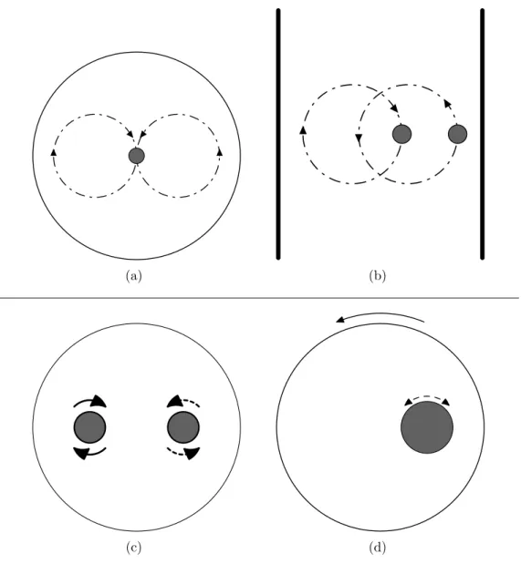
From a historical perspective, the blinking vortex flow is the first chaotic mixer ever studied. It was introduced by Aref in 1984 [8] and has received considerable attention since then [50, 69, 77]. Inside a circular domain, two point vortices are alternately switched on and off at each half-period of the stirring protocol (Fig. 2.3). The two vortices can be co- or counter- rota-tive. The flow time-dependency results from the alternation between the two stationary vortex flows. Trajectories during each half-period coincide with streamlines, which are simply circles enclosing the active vortex (see Fig. 2.1). However, trajectories jump from one streamline (corresponding to the former active vortex) to an intersecting streamline, this time corre-sponding to the new active vortex. This streamline-crossing is responsible for chaotic advection [106]. Consider for example two particles on the same streamline during one half-period: at the next blinking, they will jump to two different streamlines corresponding to different velocities, and hence separate.

Many reasons motivate the attention received by the blinking vortex flow. First, the piecewise-stationary nature of the flow provides insight into

2.1. SELECTION OF THE MIXING PROTOCOLS 33

0 ≤

_{t < T /2}

_{T /2 ≤ t < T}

Figure 2.1: Blinking vortex flow: two point vortices are alternately switched on and off. This alternation between two different stationary flows enables particles to jump between intersecting streamlines, a mechanism responsible here for fast trajectories separation, i.e. chaotic advection.

mechanisms responsible for chaotic advection, using a very simple flow: the flow complexity results only from the switching between two otherwise sim-ple stationary flows, and the consequent streamline jump. The circular nature of streamlines in the vortices’ vicinity also allows instructive ana-lytical calculation [8, 130]. Second, it is possible to derive an anaana-lytical expression for the flow created by a vortex inside a circle: this was first done by Aref [8] in a potential flow, using Milne-Thomson’s [71] circle the-orem, and extended to the Stokes flow case by Meleshko and Aref [69], who modeled the vortices by rotlets singularities. Such expressions have allowed extensive studies of particles advection in numerical simulations, such as Poincar´e sections, analysis of streamlines patterns, computation of stretch-ing coefficients, etc. Experimental realizations of the blinkstretch-ing vortex flow have also been carried out, using two fixed rotating rods as vortices [50] or magnet-driven vortices in a viscous conductive fluid [77]. The evolution of the area covered by dye has in particular been investigated in this flow [50]. However, there is a price to pay for the remarkable simplicity of the blinking vortex flow: particles initially close to one of the vortices will not much feel the effect of the other vortex, from which they are quite far (the velocity field amplitude decreases with the distance from the vortex): for a long time, these particles will effectively experience only the rotation due to one of the vortices, resulting in very poor stretching. On the other hand, particles initialized in a central region between the two vortices can easily switch between parts of the domain, because they feel the influence of

both vortices. As a result, stretching is very inhomogeneous in the blinking vortex flow.

Journal bearing flow

The journal bearing flow is also a piecewise-stationary flow. We consider the time-periodic viscous flow between two eccentric cylinders rotated al-ternately (Fig. 2.3 (d)). This flow has been much studied in the lubrication literature for the case of a thin gap between cylinders, but its first appari-tion in the chaotic advecappari-tion literature goes back to 1986 [10, 22]. Once again, streamline crossing between the two streamline patterns created by the rotating cylinders is responsible for trajectories separation and chaotic advection. In the Stokes-flow regime, trajectories are uniquely determined by the boundary displacements: journal bearing flows are therefore charac-terized by a small number of parameters, that is, cylinders radii, (positive or negative) angular displacements, and eccentricity. Numerous studies have considered different variants of this protocol [10, 22, 108, 75, 74], both nu-merically and experimentally. The existence of an analytical expression for the corresponding Stokes flow is one of the reasons accounting for the popularity of the journal bearing flow, and abundant numerical simulations aiming at characterizing phase portraits or stretching distributions have been conducted in this flow.

However, this protocol suffers from the same limitation as the blinking vortex flow: trajectories initialized close to one of the boundaries will feel only the effect of the corresponding cylinder for a long time – they may escape from this region eventually – and experience simple shear due to rotation instead of immediate exponential stretching.

Cavity flows

Another class of interesting protocols concerns cavity flows, i.e. flows inside a rectangular cavity where the top and bottom boundary are alternately horizontally driven. This well-studied [26, 61, 74] protocol has the same ad-vantages and limitations as the previously described boundary-driven pro-tocols: simple experimental realizations and analytical expression available for Stokes flow simulations, but inhomogeneous stretching.

2.1.3

Mobile boundaries vs. rod-stirring protocols

The reader might have noticed that all protocols described so far – the his-torical stirring protocols – take place in a fixed geometry, where moving

2.1. SELECTION OF THE MIXING PROTOCOLS 35

(a) (b)

Figure 2.2: Poincar´e sections for a realization of the journal bearing flow (taken from the work of Chaiken et al. [22]) (a) and figure-eight protocol (b). Many regular regions are visible in (a), whereas the chaotic region spans the entire domain in (b). As the journal bearing flow is created only by the motion of the fixed boundaries, it is in practice difficult to avoid the presence of poor-stretch regions, among which regular islands.

boundaries drag along fluid, but stay at the same position. This would be a quite non-intuitive manner to stir cake ingredients in a bowl... Every kid knows instead how to stir a cake by moving a spoon in the mixture and vis-iting every part of the bowl for a faster result. Protocols with moving rods – hence with changing geometry – are therefore good candidates for study-ing mixstudy-ing. Two reasons explain why boundary-driven protocols have been favored instead until recently. First, considering piecewise stationary pro-tocols provides an elegant representation by streamline crossing for chaotic advection, and allows for simple calculations. Moreover, closed expressions for the stirring velocity field are highly desirable for numerical simulations of particle trajectories, but the Stokes flow velocity field for one or more moving stirring rods has only been derived recently [40, 38].

However, moving rods protocols are of high interest to us, as rods can explore a large part of the fluid domain on their path, hence create more uni-form stretching. Fig. 2.2 illustrates this phenomenon: whereas a Poincar´e section of the journal bearing flow (taken from [22]) reveals a complicated structures with many elliptical islands, the chaotic region spans the entire

domain for the figure-eight protocol. Recent studies [18, 40, 38, 39, 114], on the other hand, have shown that lower boundaries on stretching could be derived from topological invariants based on the various rods crossings. Finally, keeping in mind the comparison between closed and open flows, we advocate the use of stirring-rod protocols which can be performed in closed (e.g. circular) domains as well as in open-flow channels.

2.1.4

Selected protocols

In the spirit of the previously exposed argumentation, we have mostly con-sidered rod-stirring protocols, but we have also studied historical stirring protocols such as the blinking vortex flow in numerical simulations, to bet-ter link our work to the existing libet-terature. The two stirring rods protocols studied here are show in Fig. 2.3 (a) and (b). The first protocol is the figure-eight protocol, where a single rod is moving on a figure-eight path. We have already used this protocol many times to demonstrate useful con-cepts in mixing. We use this protocol in a closed flow. The second protocol, used in an open-flow channel, is the eggbeater flow, consisting of two rods moving in a contrarotative fashion on two intersecting circles. Note that both protocols share certain similarities, as can be seen in Fig. 2.3 (a) and (b): the movement of the rod(s) imposes in both cases that fluid is sucked into a central region from the upper part of the domain, while it is pushed downwards to the sides in the lower part. These similarities will allow us to find comparable effects in closed and open flows, although we do not use exactly the same protocol.

2.2

Experimental realizations of stirring

protocols

We have built two experimental apparatus for studying mixing in closed and open flows. In both devices, we aim at measuring the concentration field resulting from the injection of a blob of dye, and its stirring and mixing by chaotic advection. Hence, we use comparable experimental methods for closed and open flows.

2.2.1

Set-up for a closed flow mixing experiment

I present here the setup of a closed-flow experiment designed to study ho-mogenization by chaotic stirring. This experimental set-up has been devised

2.2. EXPERIMENTAL SET-UP 37

(a) (b)

(c) (d)

Figure 2.3: Selected protocols: the figure-eight protocol (a) and the eggbeater protocol (b) are extensively studied in experiments and numerical computations. Comparisons are made with historical stirring protocols, that is the blinking vortex flow (c) and the journal bearing flow (d).

and built in collaboration with Natalia Kuncio during her Master’s degree internship.

The schematic drawing in Fig. 2.4 illustrates the different parts of the experiment described below.

Stirring apparatus

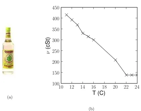
The viscous fluid used here is cane sugar syrup, aka “Canadou”, a beverage usually designed for the nobler use of lime rhum cocktails (see Fig. 2.5 (a)). For the physicist however, it has the additional advantage of being a cheap viscous Newtonian fluid. Its good optical transparency makes it also an ideal candidate for flow visualizations. Canadou viscosity measures made by Fr´ed´eric Da Cruz are shown on Fig. 2.5 (b): at room temperature (controlled at 19◦_{± 0.5}◦ _{in our laboratory), Canadou kinematic viscosity ν}

is about 250 times higher than for water.

Canadou fills a cylindrical tank (see Fig. 2.4) of 20 cm inner diameter and 10 cm height. The height of Canadou inside the tank is 9.5 cm. As the mixing pattern is visualized through the bottom of the tank, the tank is built up of a transparent plastic cylinder glued on a flat 4 mm glass plate, in order to avoid planarity defects that one can find in the bottom of a commercial glass vat. Nylon screws press the tank firmly at a fixed position against a metal frame fixed to the laboratory floor, but can also be easily removed between experiments in order to empty and clean the tank.

Canadou is stirred by a cylindrical rod plunged inside the fluid down to 1 cm of the glass plate, in order to create an approximatively 2-D flow close to the free surface 1_{. Different rod diameters (ℓ = 4, 8, 10, 12 and 16 mm)}

were used in our experiments. However, we will mostly concentrate in this manuscript on results obtained for ℓ = 16 mm. The rod is driven on a figure-eight path by an Arricks Robotics XY table that allows to control the rod movement. For each rod diameter, we performed experiments at two different linear speeds U – 1 cm_{· s}−1 _{and 2 cm· s}−1 _{– to test the influence}

of stirring speed 2_{. Depending on rod diameter and speed, we explore}

1

By visual inspection through the transparent side-wall of the vessel, we observed that dyed fluid stays in a thin layer - typically 1 or 2 mm – below the free surface. We concluded that 3-D effects are negligible for the duration of an experiment, that is about 30 stirring periods.

2_{For these low velocities, the motion of the rod is slightly jerky. However, we have} checked that the rod always comes back to the same position at the end of a cycle (up to a precision of one pixel). Moreover, in the low-Reynolds-number regime, Lagrangian trajectories depend only on the path travelled by the rod, and not of the speed at which it is travelled.

2.2. EXPERIMENTAL SET-UP 39 Camera XY table Circular neon tube FRAME Dye injection Vat Rod system

Figure 2.4: Closed-flow experimental setup. A cylindrical rod moved by a XY table stirs viscous sugar syrup inside a closed vat. At the beginning of the experiment, a spot of dye is injected just below the fluid surface. The mixing pattern is illuminated by the reflexion of a neon tube by a white plate moving with the rod, and we visualize mixing through the transparent bottom of the vat with a high-resolution digital camera.

Reynolds numbers Re = U ℓ/ν ranging from 0.16 to 1.6 . The figure-eight path is made of two adjacent circles of 6 cm diameter.

Dye injection and homogenization

Our experiments consist in visualizing the homogenization of a small blob of dyed fluid that is injected just below the fluid surface, before the rod motion starts. The dye blob is made of Indian ink (Lefranc-Bourgeois brand) diluted in Canadou (we use a 2% by volume Indian ink dilution in all experiments described in this thesis). The blob is injected at 1 mm below the surface through a syringe needle. A controllable syringe pump allows smooth injection of a fixed volume of dye (2 mL) in a reproducible fashion. Again for the sake of repeatability, two perpendicular sliding tracks (see Fig. 2.4) allow to inject the blob always at the same place. Indian ink, hence dye, is lighter than Canadou: the buoyancy force thus lifts the blob

(a)

(b)

Figure 2.5: (a) Cane sugar syrup, aka Canadou, is cheap and easily commercially available. Its basic fabrication principle consists in slowly incorporating cane sugar in warm water. (b) Canadou kinematical viscosity (measures by Fr´ed´eric da Cruz) vs. temperature. At 19◦_{C, Canadou is about 250 times more viscous}

than water.

to the free surface, ensuring that the initial condition is two-dimensional, with dye confined to a thin upper layer.

The choice of Indian ink was motivated by its great dyeing intensity: little dye is required to color a great quantity of Canadou, so that we might hope that dyed fluid has the same hydrodynamical properties as unmarked fluid. However, commercial Indian ink is made of an aqueous suspension of black carbon particles, stabilized by a binder, usually polymers which are responsible for the ink’s very low surface tension. As a result, blobs with a high ink concentration tend to break up as they reach the surface, to minimize the surface tension. We therefore limit ourselves to a highly diluted ink solution, where this effect is not visible on the experiment’s timescale.

2.2. EXPERIMENTAL SET-UP 41

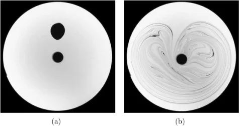
(a) (b)

Figure 2.6: (a) Initial condition: a small blob of marked fluid is released just under the free surface. (b) We follow the evolution of the mixing pattern imposed by the stirring rod.

Data acquisition

Our primary goal is to follow the evolution of the dye concentration field as the mixing process goes on. To do so, we need to access the concentration field through the greyscale intensity of pictures of the mixing pattern, in order to have an unambiguous relation between greyscale intensity and dye concentration. It is important to note that this condition imposes the use of transmission lighting. Since we observe the mixing pattern from below, all light rays must therefore come from above. Because of the XY table mechanical device, there is no room left for a light source above the fluid tank. Our light source is therefore an indirect one: a large plastic plate coated with white paint is fixed between the rod and the XY table carriage. The white plate is illuminated by a circular neon tube around the cylindrical tank (see Fig. 2.4). The inner tank border is coated with matted black film to ensure that only light reflected by the white plate can illuminate the fluid. A digital Canon EOS Mark II 1-D color camera is used to take 12 bit, 3504×2336 pictures at a fixed rate. Depending on rod velocity, we take 3 (U = 2 cm_{· s}−1_{) or 6 (U = 1 cm· s}−1_{) pictures per stirring period. We also}

wrap the camera in a black-cloth dark room fixed to the tank glass plate and the metallic frame to avoid any unwanted lighting of the apparatus.