Orbital forcings of the Earth?s climate in wavelet domain

(1)

HAL Id: hal-00298116

https://hal.archives-ouvertes.fr/hal-00298116

Submitted on 23 Sep 2005

HAL is a multi-disciplinary open access

archive for the deposit and dissemination of sci-entific research documents, whether they are pub-lished or not. The documents may come from teaching and research institutions in France or abroad, or from public or private research centers.

L’archive ouverte pluridisciplinaire HAL, est destinée au dépôt et à la diffusion de documents scientifiques de niveau recherche, publiés ou non, émanant des établissements d’enseignement et de recherche français ou étrangers, des laboratoires publics ou privés.

Orbital forcings of the Earth?s climate in wavelet

domain

A. V. Glushkov, V. N. Khokhlov, N. S. Loboda, V. D. Rusov, V. N. Vaschenko

To cite this version:

A. V. Glushkov, V. N. Khokhlov, N. S. Loboda, V. D. Rusov, V. N. Vaschenko. Orbital forcings of the Earth?s climate in wavelet domain. Climate of the Past Discussions, European Geosciences Union (EGU), 2005, 1 (2), pp.193-214. �hal-00298116�

(2)

CPD

1, 193–214, 2005

Orbital forcings of the Earth’s climate in

wavelet domain A. V. Glushkov et al. Title Page Abstract Introduction Conclusions References Tables Figures J I J I Back Close

Full Screen / Esc

Print Version Interactive Discussion

EGU

Climate of the Past Discussions, 1, 193–214, 2005 www.climate-of-the-past.net/cpd/1/193/

SRef-ID: 1814-9359/cpd/2005-1-193 European Geosciences Union

Climate of the Past Discussions

Climate of the Past Discussions is the access reviewed discussion forum of Climate of the Past

Orbital forcings of the Earth’s climate in

wavelet domain

A. V. Glushkov1, V. N. Khokhlov2, N. S. Loboda2, V. D. Rusov3, and V. N. Vaschenko4

1

Institute for Applied Mathematics, Department of Computational Mathematics, Odessa, Ukraine

2

Innovative Geosciences Research Centre, Department of Hydrometeorology, Odessa, Ukraine

3

Odessa National Polytechnic University, Department of Theoretical Physics, Odessa, Ukraine

4

Kiev National University, Department of Antarctic Sciences, Kiev, Ukraine

Received: 3 August 2005 – Accepted: 9 September 2005 – Published: 23 September 2005 Correspondence to: V. N. Khokhlov (vkhokhlov@ukr.net)

(3)

CPD

1, 193–214, 2005

Full Screen / Esc

EGU

Abstract

We examine two paleoclimate proxy records – the temperature differences from the Antarctic Vostok ice core and the composite δ18O record from three sites (V19-30, ODP 677, and ODP 846) – in order to search for indications of orbital forcings. We demonstrate that the non-decimated wavelet transform is an appropriate tool for

in-5

vestigating temporarily changing spectral properties of records. Our results indicate that abrupt climate warmings with cyclicity of ∼100 kiloyears during the last 400 kilo-years were caused by the combined unidirectional influences of three orbital parame-ters and the eccentricity can be considered as a modulator defining transitions from the Ice Ages to the periods of comparative warmings. Non-decimated wavelet transform

10

avails discovering the possible part played in climate change by the eccentricity-forced variations. Up to approximately 1.7 million years BP, the influence of this variations of eccentricity appears in increasing for almost all local maxima of δ18O. Since the ∼1.7 million years BP, minor and significant maxima alternated and this not affected as much the variations of δ18O.

15

1. Introduction

In spite of the fact that during the past decade many researches had attended to climate variations at time scales exceeding the 10 kiloyears (hereafter, we use the denotation of ‘ky’), the mechanisms which cause those climate variations are not well understood. Nevertheless, most investigators agree in opinion that some external forcing, not the

20

internal dynamics, can be considered as the trigger factor for the low-frequency al-ternation of cold and warm periods in the Earth’s climate. Among the most significant extraterrestrial factors, the variations of insolation and galactic cosmic rays are notable; the influence of the latter is not well studied.

If not consider annual variations, the forcing of the temperature changes by the

fluc-25

(4)

CPD

1, 193–214, 2005

Full Screen / Esc

EGU

ky. Some recent studies (e.g. Oh et al., 2002; Dima et al., 2005) had showed that well-known cycles of solar activity such as the ∼11 year Schwabe (sunspot) cycle and the ∼76–90 year Gleissberg cycle are reflected in the surface climate. Moreover, the reduced solar activity and low number of sunspots are considered one of the reasons of the Maunder Minimum (1645–1715). Solar activity during this period was near its

5

lowest levels of the past 8 ky (Lean and Rind,1999). van Geel et al.(1999) had sup-posed that the ∼1450 year cycle (the Maunder Minimum delineates the coldest phase of such periodicity) is also solar-induced.

In comparison with above mentioned periodicities, the fluctuations of paleoparame-ters forced by the changes of the Earth’s orbital paramepaleoparame-ters appear more appreciable.

10

It is well known from many studies (e.g.Muller and MacDonald,1997a;Ridgwell et al., 1999;Petit et al.,1999;Wunsch,2003;Berger and Loutre,2004; EPICA,2004) that during approximately the past million years various paleorecords are dominated by the ∼100 ky cycle, whereas a few preceding millions years are characterized by the ∼41 ky cycle. A linkage between orbital parameters and climate is provided by the Milankovitch

15

theory, which states that melting of the northern ice sheets is driven by peaks in North-ern Hemisphere summer insolation. However, as better data have become available, difficulties have arisen with the Milankovitch theory. The insolation includes the ∼41 ky cycle but no significant ∼100 ky variations. Moreover, an expected ∼400 ky cycle is not observed. The modulation of the ∼100 ky cycles does not follow the expected pattern –

20

a disagreement known as the ‘Stage-11 problem’, when a major glacial termination oc-curred during a period of minor insolation changes around ∼400 ky BP (before present) (Imbrie et al.,1993). High-resolution spectral analysis of the glacial records shows a narrow ∼100 kyr cycle, in conflict with the double peak expected from the Milankovitch theory (Muller and MacDonald,1997b). Finally, the penultimate glacial termination

ap-25

pears to have preceded the insolation increase that is supposed to have caused it – a conflict known as the ‘causality problem’. These uncertainties support still steadfast attention to the low-frequency climate change.

(5)

cyclic-CPD

1, 193–214, 2005

Full Screen / Esc

EGU

ity use the Fourier transform to paleorecords. Fourier transform extracts details from the signal frequency, but all information about the location of a particular frequency within the signal is lost. During last two decades, many scientists had used the new powerful tool based on the wavelet decomposition for analyzing various signals includ-ing time series of paleoparameters (Lin and Chao, 1998; Guyodo et al., 2000;

Har-5

greaves and Abe-Ouchi, 2003; Valet, 2003; Witt and Schumann, 2005); in the latter case the continuous wavelet transform was usually used. In this article, we work with non-decimated (discrete) wavelet transform rather than continuous wavelet transform, because from a statistical point of view, they are well adapted (i.e. search for corre-lations or noise reduction) and offer a very flexible tool for analysis of discrete time

10

series such as the ones under study here. The advantages of non-decimated wavelet transform also include (1) a much better temporal resolution at coarser scales than with ordinary discrete wavelet transform, and (2) it allows us to isolate time series of the major components of meteorological signals in a direct way. Similar approach had been successfully applied to some other climatic time series (Oh et al.,2002;Khokhlov

15

et al.,2004;Loboda et al.,2005).

The intention of this paper is to examine two time series of paleoparameters (the temperature differences from the Antarctic Vostok ice core and the composite δ18O record from three sites (V19-30, ODP 677, and ODP 846) in order to search for indi-cations of orbital forcings. Since the amplitude of these parameters cannot assumed

20

to be constant, the non-decimated wavelet transform, which allows a simultaneous decomposition in time and frequency domain, is applied. This paper is organized as follows. First general information on orbital forcings of climate is cited. Further, both the approach used the non-decimated wavelet transform and the data used are briefly described. The results of wavelet transform for the paleoparameters are presented and

25

(6)

CPD

1, 193–214, 2005

Full Screen / Esc

EGU

2. Change of orbital parameters and climate

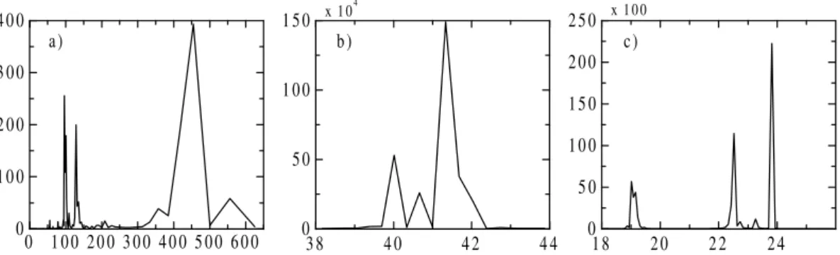
As stated above, the fluctuations of orbital parameters can force the climate variations. First, let us describe in a general way this forcing. To illustrate the most appreciable periodicities of the orbital parameters, we apply the Fourier transform to the data of Berger and Loutre(1991); the results are shown in Fig.1.

5

The planet describes ellipse in the field of central forces. The plane of elliptical orbit is referred as the ecliptic. The shape of this orbit is characterized by the eccentricity. The Earth’s movement along the heliocentric orbit is disturbed by other planets and depends on certain factors. The ecliptic remains invariable due to these non-central disturbances, but eccentricity varies. These variations are ranged between 0.000515

10

and 0.057118 during the past five millions years (Berger and Loutre,1991) and are not described by harmonic oscillations but are the frequency spectrum with the predomi-nant periods of the 100, 128, and 454 ky (Fig.1a). The amount of energy incoming into upper atmosphere differs in 0.1 percents between the cases of near-circular orbit and maximal eccentricity. This value suffices to change considerably (from climatic point of

15

view) the surface temperature that causes in turn extreme climatic conditions. In the case when the winter (e.g., in the Northern Hemisphere) falls on the perihelion, the cold period is shorter. This case takes place at present and Northern winters are shorter and wormer than Southern winters. For the case of near-circular orbit (minimum of eccentricity), the duration of winter is almost equal in both hemispheres.

20

The angular momentum of the Earth’s rotation is not staying due to the interaction of the Sun and the Moon with the quadrupole moment of the Earth’s rotation. Conse-quently, the orientation of the axis of the equator varies with respect to the system of fixed stars. Such variations can be considered from point of view of two processes – changes of obliquity and precession.

25

The obliquity is the angle included between the plane of the Earth’s equator and the ecliptic. For the past five millions years the obliquity is ranged from 22.1 to 24.5 degrees with the period of the 41 ky approximately (Fig.1b). The obliquity not affects

(7)

CPD

1, 193–214, 2005

Full Screen / Esc

EGU

the total insolation but defines seasonal variations of temperature which enlarge as the obliquity increases. This effect appears synchronously for both hemispheres and increases with respect to geographical latitudes. During periods with low seasonal variations of temperature, the ice lumps can be generated in winters and their slow melting during the warm half of year can causes the glaciations. On the other hand,

5

during periods with high seasonal variations of temperature the ice cover growing in the winter melts in the summer. Thus, the coarse correlation between the periods of low and high insolation contrasts, on the one hand, and the alternation of glacial and interglacial periods, on the other hand, can be ascertained.

The precession is the fluctuations of the axis of the equator around the pole of

eclip-10

tic. These fluctuations have very complicated nature and can not be described by the harmonic law even though with rough approximation in contrast to two other orbital parameters. Its frequency spectrum is divided into bands with periods of the 19, 22, and 24 ky approximately (Fig. 1c). The precession defines the equinox shift and not causes any annual insolation variation. Therefore, it not affects the seasonal variations

15

of temperature in the case of circular orbit but such forcing exists in the case of elliptical orbit, at that this effect increases when the eccentricity enlarging.

Thus the changes of the Northern and Southern seasonal temperatures stipulated by the obliquity are in-phase and not depend on the eccentricity. Conversely, similar changes due to the precession are in opposite phase and increase when the

eccentric-20

ity enlarging. Furthermore, the observed low-frequency variations of paleoparameters must depend on compound effect of the three orbital parameters not single one. To illustrate such a compound effect, we apply the non-decimated wavelet transform to the time series of paleoparameters.

3. Data and method used

25

To study the impact of orbital parameters changes, we use two paleoreconstruction with different origin. First we use the temperature differences with respect to mean modern

(8)

CPD

1, 193–214, 2005

Full Screen / Esc

EGU

value obtained by using the deuterium data from the Antarctic Vostok ice core (Petit et al.,1999). This temperature is calculated using a deuterium/temperature gradient of 9%/◦C after accounting for the isotopic change of sea-water (see Jouzel et al.,1996, for details). Second dataset under consideration is the composite record of oxygen isotope ratios, δ18O, of benthic foraminifera from sediment cores of V19-30, ODP 677,

5

and ODP 846 sites (Shackleton,1995). The compositing of data from these cores is possible due to the sites are nearly situated. Information on the geographic coordinates and time domain of these sites is presented in Table 1. The physical basis for proxy climate measurements from the stable18O isotope is that the vapour pressure of H₂18O is lower than that of H₂16O. Evaporation from the oceans thus produces water vapour

10

that is18O-depleted (by about 1% relative). The relative proportion of18O in a sample is expressed in terms of its fractional deviation, δ18O, from a standard mean ocean water value (about 2·10−3). The δ18O value of sea sediments provides a measure of the global volume of water locked up in (18O-depleted) ice sheets, since high ice volumes leave the oceans enriched in18O.

15

Since the time interval between the terms of series is unequal, we use the piecewise cubic Hermite interpolating polynomial (Kahaner et al.,1988) to prepare input data for wavelet transform. Note that our attempt using the spline interpolation was unsuccess-ful due to abnormal large local extremes in the interpolated time series.

Le us here describe briefly the methodology of non-decimated wavelet transform; for

20

detail about wavelet theory, the monographs ofDaubechies(1992) andGoswami and Chan (1999) can be recommended.

The dilation and translation of one mother wavelet ψ (t) generates the wavelet ψ_j,k(t)=2j /2ψ (2jt−k), where j, k∈Z. The dilation parameter j controls how large the wavelet is, and the translation parameter k controls how the wavelet is shifted along

25

the t-axis. For a suitably chosen mother wavelet ψ (t), the set {ψ_j,k}_j,k provides an orthogonal basis, and the function f which is defined on the whole real line can be

(9)

CPD

1, 193–214, 2005

Full Screen / Esc

Print Version Interactive Discussion EGU expanded as f (t)= ∞ X k=−∞ c_0,kφ_0,k(t)+ J X j=1 ∞ X k=−∞ d_{j k}ψ_j,k(t), (1)

where φ₀ is the scaling function or so-called ‘father’ wavelet, the maximum scale J is determined by the number of data, the coefficients c_0k represent the lowest frequency smooth components, and the coefficients d_{j k}deliver information about the behaviour of

5

the function f concentrating on effects of scale around 2j near time k × 2j. This wavelet expansion of a function is closely related to the discrete wavelet transform (DWT) of a signal observed at discrete points in time.

In practice, the length of the signal, say n, is finite and, for our study, the data are available discretely, i.e. the function f (t) in Eq. (1) is now a vector f=(f (t₁), . . . , f (t_n))

10

with t_i=i/n and i=1, . . . , n. With these notations, the DWT of a vector f is simply a matrix product d=Wf, where d is an n×1 vector of discrete wavelet coefficients indexed by 2 integers, d_{j k}, and W is an orthogonal n×n matrix associated with the wavelet

basis. The DWT is quickly computed through an efficient algorithm developed byMallat (1989). For computational reasons, it is simpler to perform the wavelet transform on

15

time series of dyadic (power of 2) length.

One particular problem with DWT is that, unlike the discrete Fourier transform, it is not translation invariant. This can lead to Gibbs-type phenomena and other arte-facts in the reconstruction of a function. The non-decimated wavelet transform (NWT) of the data (f (t₁), . . . , f (t_n)) at equally spaced points t_i=i/n is defined as the set of

20

all DWT’s formed from the n possible shifts of the data by amounts i /n, i=1, . . . , n. Thus, unlike the DWT, there are 2j coefficients on the jth resolution level, there are n equally spaced wavelet coefficients in the NWT: d_{j k}=n−1Pn

i=12 j /2

ψ [2j(i /n−k/n)]y_i, k=0, . . . , n−1, on each resolution level j. This results in log₂(n) coefficients at each location. As an immediate consequence, the NWT becomes translation invariant. Due

25

(10)

CPD

1, 193–214, 2005

Full Screen / Esc

EGU

better exploratory tool for analyzing changes in the scale (frequency) behaviour of the underlying signal in time. These advantages of the NWT over the DWT in time series analysis are demonstrated inNason et al.(2000).

From the above paragraphs, it is easy to plot any time series into the wavelet domain. Another way of viewing the result of a NWT is to represent the temporal evolution of

5

the data at a given scale. This type of representation is very useful to compare the temporal variation between different time series at a given scale. To obtain such results, the smooth signal S0 and the detail signals D_j (j=1, . . . , J) are defined as follows S₀(t)= ∞ X k=−∞ c_0kφ_0,k(t), D_j(t)= ∞ X k=−∞ d_{j k}ψ_j,k(t). (2)

Sequentially, the temporal multi-resolution decomposition of a signal is derived from

10

D_j₋₁(t)= S_j(t) − S_j₋₁(t).

The fine scale features (high frequency oscillations) are captured mainly by the fine scale detail components D_J and D_J₋₁. The coarse scale components S₀, D₁, and D₂ correspond to lower frequency oscillations of the signal. Note that each band is equivalent to a band-pass filter.

15

Further we use the Daubechies wavelet (db15) as mother wavelet. This wavelet is biorthogonal and supports discrete wavelet transform (Daubechies,1992). The choice of mother wavelet was realized by the estimation of Shannon enthropy (Coifman and Wickerhauser,1992).

4. Wavelet decomposition of paleoparameters

20

4.1. Temperature reconstructed from Antarctic Vostok ice core

Non-decimated wavelet transform of temperature differences from the Antarctic Vos-tok ice core provides the ten detail components. Among these components, three

(11)

CPD

1, 193–214, 2005

Full Screen / Esc

EGU

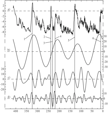
ones – D₃, D₅, and D₆ – have the periods of ∼100, 40, and 20 ky, respectively. Thus the wavelet decomposition extracts three signals with periods, which correspond to the variations of above-mentioned orbital parameters, i.e. to the eccentricity, obliquity, and precession, respectively. Note that the correlation coefficients between these sig-nals and time series of orbital parameters during last 420 ky exceed the value of 0.7.

5

Figure 2 shows the original time series of temperature differences and three detail components.

One can be foremost noted that the variations of temperature forced by the eccen-tricity appear responsible for the alternation of glacial and interglacial periods in the Earth’s climate. However, abrupt warmings are caused by all three orbital

parame-10

ters (vertical lines 1, 5 and 6 in Fig. 2). Subsequent as many abrupt transitions to the Ice Ages are stimulated by the decreases of temperature forced by the obliquity and precession in spite of the fact that the eccentricity contributes to the increase of temperature. The warming period of 250–200 ky BP can be considered as an inter-esting illustration for such ambiguous triple contribution. This warming was observed

15

somewhat earlier than the eccentricity-stipulated temperature maximum (vertical line 2 in Fig. 2) and was caused by the influence of other orbital parameters. However, the rise of temperature ended abnormally rapidly that arose from the forcing of both the obliquity and the precession (vertical line 3 in Fig. 2). Somewhat later on, when the influence of all three orbital parameters combined (vertical line 4 in Fig.2), the abrupt

20

tendency to the climate worming was observed. Note that the analogous temperature change can be found in the ice core record from Dome C, Antarctica (EPICA,2004).

Thus, the fact that the periods of abrupt climate warmings with cyclicity of ∼100 ky during the last 400 ky were caused by the combined unidirectional influences of three orbital parameters can be considered as the main outcome of above analysis.

Fur-25

thermore, during the last 400 ky the eccentricity can be considered as a modulator defining transitions from the Ice Ages to the periods of comparative warmings. Both the obliquity- and the precession-caused variations of temperature are imposed on the eccentricity-modulated temperature change, but not able themselves produce abrupt

(12)

CPD

1, 193–214, 2005

Full Screen / Esc

EGU

warmings. Therefore this triple influence can be considered as a reason for the unequal duration of the longer Ice Ages and the shorter warmings during the last 400 ky. 4.2. Composite oxygen isotope ratios from the V19-30, ODP 677, and ODP 846 sites Before applying wavelet decomposition to the time series of oxygen isotope ratios, δ18O, let us make some remarks on predominant periodicities in the climate change

5

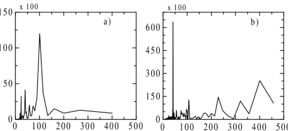
during the past several million years. It is well-know that the late million years is char-acterized by the so-called Mid-Pleistocene transition of the Earths climate with a shift towards much larger Northern ice shields at ∼920 ky BP and the predominance of ∼100 ky ice age ciclicity. To illustrate the latter, we apply the Fourier transform to the 4000-ky composite record of oxygen isotope ratios for two periods – first one starts

10

since 780 ky BP up to the present and second one embraces the period of 4000–780 ky BP. The choice of of separating value is defined by so-called Brunhes-Matuyama mag-netic reversal in the δ18O time series (Bassinot et al.,1994). Figure3shows the results of this transform.

During the last 780 ky (Fig. 3a), the variations of δ18O with the period of ∼100 ky

15

(eccentricity-forced) are predominant, whereas the powers for the 40 ky (obliquity-forced) and 23.5 ky (precession-(obliquity-forced) are 3–4 times as less. Over the period an-tecedent to the Brunhes-Matuyama boundary age (Fig. 3b), the 41-ky period was a cause for most of climate changes; the strength of this periodicities enlarges 15 times as much in comparison with posterior period. On the other hand, the strength of

max-20

imum on the ∼100 ky is almost staying for the both periods. In contrast to the later period, the maximum at the ∼400 ky can be found with the 2.5 times as less power in comparison with the obliquity-forced fluctuations of δ18O. Regardless of the fact that during the period antecedent to the Brunhes-Matuyama boundary age the climate changes appear obliquity-forced, they can not be explained only this factor just as the

25

eccentricity only can not be considered the cause of ice age-warming alternations dur-ing the later period. From our point of view, the non-decimated wavelet transform avails discovering the low-frequency components in details.

(13)

CPD

1, 193–214, 2005

Full Screen / Esc

EGU

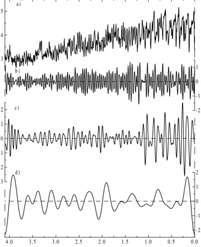
Figure 4shows the original time series of δ18O and three detail components – D₈, D₇, and D₅. The period of detail component D₈ is around 40 ky, i.e. this component displays the climate change caused by the obliquity variations. For the detail com-ponent D₇, the period is ∼100 ky and the changes of δ18O represent the eccentricity variations, as well as the detail component D₅, but the latter is characterized by the

5

periodicity of ∼400 ky.

During the last 4 million years, the oxygen isotope ratios tended to increasing. The period of 40 ky was predominant up to the ∼1 million years BP, but during the last million years the 100-ky periodicity was most prominent. Moreover, the amplitude of the latter increases, at that the robust bound observes at the ∼1 million years BP, since

10

which the transition occurs to the eccentricity-forced variations.

As regards the eccentricity-forced climate change with the period of ∼400 ky, the robust change of amplitude occurred at approximately 1.7 million years BP. Up to this bound, the influence of this variations of eccentricity appears in increasing for almost all local maxima of δ18O (compare the upper and lower graphs in Fig. 4). Since the

15

∼1.7 million years BP, minor and significant maxima alternated and this not affected as much the variations of δ18O.

5. Discussion

As it was declared in Sect. 1, present paper is aimed at the searching for orbital in-dicators in paleorecords really, rather than at the revision of present opinion on the

20

Milankovitch theory of Ice Ages. From this point of view, the non-decimated wavelet transform is the excellent tool allowed the identification of low-frequency detail com-ponents in two paleorecords with different origins. The results adduced in this study can be evidence of advantage for this method, namely its flexibility in the adjustment to the local changes in the period of paleoparameters, which are wide-ranging. Since

25

wavelets support clear minima and maxima they take into account realistic estimations of cycle-length.

(14)

CPD

1, 193–214, 2005

Full Screen / Esc

EGU

Nevertheless, our results could not explain absolutely all variations observed in the original time series of paleoparameters. This can be related to the variations in both low- and high-frequency domains, which are not referred to the orbital forcing. Even though the time interval between values in time series is equal to the 0.3 ky, as it is accepted in this study, high-frequency variations can not be completely ignored.

5

Some recent studies showed that the processes taking place in the atmosphere-ocean-ice sheets system manifest themselves substantially in the response of climatic system on the variations of insolation. By using the numerical simulations with cou-pled atmosphere-ocean general circulation mode, Hall et al. (2005) showed that the model’s response conforms to Milankovitch’s hypothesis during the Northern summer

10

only, whereas most of the simulated orbital signatures in wintertime surface air tem-perature over midlatitude continents are directly traceable not to local radiative forcing, but to orbital excitation of the Northern Annular Mode. On the other hand, the 11-year solar cycle could influence tropospheric climate through an indirect pathway: tropical stratospheric ozone heating creates off-equatorial circulation anomalies, and

subse-15

quent interactions with planetary-scale Rossby waves bring the anomalies poleward and downward in the winter hemisphere (Baldwin and Dunkerton,2005). Also, rapid fluctuations of the southern margin of the Laurentide ice sheet in the Great Lakes re-gion of North America may be an important triggering mechanism of millennial-scale climatic changes in the North Atlantic and Arctic Oceans (Nesje et al.,2004).

20

The above-mentioned information can be considered as indirect evidence that a por-tion of solar- and orbital-induced climate changes could become apparent some time after. Such a delay could be, very likely, a few kiloyears, especially in the case of such inertial systems as the ocean or ice sheets. The estimation of this ambiguous delay is the difficult task.

25

As regards the low-frequency variations with the periods comparable to the changes of orbital parameters, let us consider briefly the periodicities of 100–400 ky only. Fig-ure 3b shows that Fourier spectrum has two maxima at the 230 and 320 ky, which can not be explained by the orbital-forcing. The most appropriate to this periodicity is the

(15)

CPD

1, 193–214, 2005

Full Screen / Esc

EGU

average duration of geomagnetic polarity intervals, but there is a wide range of dura-tions with the shorter duration intervals being more common. From the other hand, the two ages mentioned in Section 4.2, the ∼1 and ∼1.7 million years BP, correspond sufficiently to the two paleomagnetic events – the Jaramillo and Olduvai, respectively. It is well known that the magnetic properties of a sediment, including mineralogy, grain

5

size, and concentration of magnetic minerals can be strongly related to climatic forc-ing (Valet,2003). Two studies with the data from ODP Site 983 (Channell and Kleiven, 2000;Guyodo et al.,2000) had showed the existence of periodic signals embedded into the paleointensity record during the last 1.1 million years. These signals correspond to the Earth orbital eccentricity, obliquity, and precession. However, the significant

rela-10

tionship is observed over some periods of time.

So, the paleorecords can be affected by the system of quasi-linear and non-linear effects. The non-decimated wavelet transform can be considered as a tool permitting the extracting some from these effects. In the present paper, we used successfully this method to extract the orbital fingerprints in the two paleoparameters.

15

References

Baldwin, M. P. and Dunkerton, T. J.: The solar cycle and stratosphere–troposphere dynamical coupling, J. Atmos. Solar-Terr. Phys., 67, 71–82, 2005. 205

Bassinot, F. C., Labeyrie, L. D., Vincent, E., Quidelleur, X., Shackleton, N. J., and Lancelot, Y.: The astronomical theory of climate and the age of the Brunhes-Matuyama magnetic reversal,

20

Earth Planet. Sci. Lett., 126, 91–108, 1994. 203

Berger, A. and Loutre, M. F.: Insolation values for the climate of the last 10 million of years, Quatern. Sci. Rev., 10, 297–317, 1991. 197,211

Berger, A. and Loutre, M. F.: Astronomical theory of climate change, J. Phys. IV France, 121, 1–35, 2004. 195

25

Channell, J. E. T. and Kleiven, H. F.: Geomagnetic palaeointensities and astrochronological ages for the Matuyama-Brunhes boundary and the boundaries of the Jaramillo Subchron:

(16)

CPD

1, 193–214, 2005

Full Screen / Esc

EGU

palaeomagnetic and oxygen isotope records from ODP Site 983, Phil. Trans. R. Soc. Lond. A, 358, 1027–1047, 2000. 206

Coifman, R. R. and Wickerhauser, M. V.: Entropy-based Algorithms for best basis selection, IEEE Trans. Inf. Theory, 38, 713–718, 1992. 201

Daubechies, I.: Ten lectures on wavelets, SIAM, Philadelphia, 1992. 199,201

5

Dima, M., Lohmann, G., and Dima, I.: Solar-induced and internal climate variability at decadal time scales, Int. J. Climatol., 25, 713–733, 2005. 195

EPICA community members: Eight glacial cycles from an Antarctic, Nature, 429, 623–628, 2004. 195,202

Goswami, J. C. and Chan, A. K.: Fundamentals of wavelets, Theory, algorithms, and

applica-10

tions, Wiley-Intercsience, New York, 1999. 199

Guyodo, Y., Gaillot, P., and Channell J. E. T.: Wavelet analysis of relative geomagnetic paleoin-tensity at ODP Site 983, Earth Planet. Sci. Lett., 184, 109–123, 2000. 196,206

Hall, A., Clement, A., Thompson, D. W. J., Broccoli, A., and Jackson, C.: The importance of atmospheric dynamics in the Northern Hemisphere wintertime climate response to changes

15

in the Earth’s orbit, J. Climate, 18, 1315–1325, 2005. 205

Hargreaves, J. C. and Abe-Ouchi, A.: Timing of ice-age terminations determined by wavelet methods, Paleoceanography, 18, 1035, doi:10.1029/2002PA000825, 2003. 196

Imbrie, J., Berger, A., Boyle, E. A., Clemens, S. C., Duffy, A., Howard, W. R., Kukla, G., Kutzbach, J., Martinson, D. G., McIntyre, A. C., Mix, A. C., Molfino, B., Morley, J. J.,

Pe-20

terson, L. C., Pisias, W. L., Prell, W. L., Raymo, M. E., Shackleton, N. J., and Toggweiler, J. R.: On the structure and origin of major glaciation cycles: 2. The 100 000-year cycle, Paleoceanography, 8, 699–735, 1993. 195

Jouzel, J., Waelbroeck, C., Malaiz ´e, B., Bender, M., Petit, J. R., Barkov, N. I., Barnola, J. M., King, T., Kotlyakov, V. M., Lipenkov, V., Lorius, C., Raynaud, D., Ritz, C., and Sowers, T.:

25

Climatic interpretation of the recently extended Vostok ice records, Clim. Dyn., 12, 513–521, 1996. 199

Kahaner, D., Moler, C., and Nash, S.: Numerical methods and software, Prentice Hall, Upper Saddle River, NJ, 1988. 199

Khokhlov, V. N., Glushkov, A. V., and Tsenenko, I. A.: Atmospheric teleconnection patterns and

30

eddy kinetic energy content: wavelet analysis, Nonlin. Processes Geophys., 11, 295–301, 2004,

(17)

CPD

1, 193–214, 2005

Full Screen / Esc

EGU

Lean, J. and Rind, D.: Evaluating sun-climate relationships since the Little Ice Age, J. Atmos. Solar-Terr. Phys., 61, 25–36, 1999. 195

Lin, H.-S. and Chao, B. F.: Wavelet spectral analysis of the Earth’s orbital variations and pale-oclimatic cycles, J. Atmos. Sci., 55, 227–236, 1998. 196

Lododa, N. S., Glushkov, A. V., Khokhlov, V. N., and Lovett, L.: Using non-decimated

5

wavelet decomposition to analyse time variations of North Atlantic Oscillation, eddy ki-netic energy, and Ukrainian precipitation, J. Hydrol., corrected proof available online, doi:10.1016/j.jhydrol.2005.02.029, 2005. 196

Mallat, S.: A theory for multiresolution signal decomposition: the wavelet representation, IEEE Trans. Patt. Anal. Mach. Intell., 11, 674–693, 1989. 200

10

Muller, R. A. and MacDonald, G. J.: Simultaneous presence of orbital Inclination and eccentric-ity in proxy climate records from Ocean Drilling Program Site 806, Geology, 25, 3–6, 1997a.

195

Muller, R. A. and MacDonald G. J.: Glacial cycles and astronomical forcing, Science, 277, 215–218, 1997b. 195

15

Nason, G., von Sachs, R., and Kroisand, G.: Wavelet processes and adaptive estimation of the evolutionary wavelet spectrum, J. R. Stat. Soc., B 62, 271–292, 2000. 201

Nesje, A., Dahl, S. O., and Bakke, J.: Were abrupt Lateglacial and early-Holocene climatic changes in northwest Europe linked to freshwater outbursts to the North Atlantic and Arctic Oceans?, The Holocene, 14, 299–310, 2004. 205

20

Oh, H.-S., Ammann, C. M., Naveau, P., Nychka, D., and Otto-Bliesner, B. L.: Multi-resolution time series analysis applied to solar irradiance and climate reconstructions, J. Atmos. Solar-Terr. Phys., 65, 191–201, 2003. 195,196

Petit, J. R., Jouzel, J., Raynaud, D., Barkov, N. I., Barnola, J. M., Basile, I., Bender, M., Chap-pellaz, J., Davis, J., Delaygue, G., Delmotte, M., Kotlyakov, V. M., Legrand, M., Lipenkov, V.,

25

Lorius, C., Pepin, L., Ritz, C., Saltzman, E., and Stievenard, M.: Climate and atmospheric history of the past 420 000 years from the Vostok Ice Core, Antarctica, Nature, 399, 429–436, 1999. 195,199

Ridgwell, A. J., Watson, A. J., and Raymo, M. E.: Is the spectral signature of the 100 kyr glacial cycle consistent with a Milankovitch origin?, Paleoceanography, 14, 437–440, 1999. 195

30

Shackleton, N. J.: New data on the evolution of Pliocene climatic variability, in: Paleoclimate and evolution with emphasis on human origins, edited by: Vrba, E. S., Denton, G. H., Partridge, T. C., and Burckel, L. H., Yale University Press, 242–248, 1995. 199

(18)

CPD

1, 193–214, 2005

Full Screen / Esc

EGU

Valet, J.-P.: The variations in geomagnetic intensity, Rev. Geophys., 41, 1/1004, doi:10.1029/2001RG000104, 2003. 196,206

van Geel, B., Raspopov, O. M., Renssen, H., van der Plicht, J., Dergachev, V. A., and Meijer, H. A. J.: The role of solar forcing upon climate change, Quater. Sci. Rev., 18, 331–338, 1999.

195

5

Witt, A. and Schumann, A. Y.: Holocene climate variability on millennial scales recorded in Greenland ice cores, Nonlin. Processes Geophys., 12, 345–352, 2005,

SRef-ID: 1607-7946/npg/2005-12-345. 196

Wunsch, C.: The spectral description of climate change including the 100 ky energy, Clim. Dyn., 20, 353–363, 2003. 195

(19)

CPD

1, 193–214, 2005

Full Screen / Esc

EGU

Table 1. Location and age of sediments for V19-30, ODP 677, and ODP 846 sites.

V19-30 ODP 677 ODP 846 Latitude (S) 3◦230 1◦120 3◦060 Longitude (W) 83◦310 83◦440 90◦490 Age (ky) 0–340 340–1811 1811–8350

(20)

CPD

1, 193–214, 2005

Full Screen / Esc

Print Version Interactive Discussion EGU 0 1 0 0 2 0 0 3 0 0 4 0 0 5 0 0 6 0 0 0 1 0 0 2 0 0 3 0 0 4 0 0 a ) 3 8 4 0 4 2 4 4 0 5 0 1 0 0 1 5 0 1 8 2 0 2 2 2 4 0 5 0 1 0 0 1 5 0 2 0 0 2 5 0 b ) c ) x 1 04 x 1 0 0

Fig. 1. Fourier power spectrum of the orbital parameter data fromBerger and Loutre(1991):

(a) eccentricity, (b) obliquity, and (c) precession. Y-axis is the power and x-axis is the period in

(21)

CPD

1, 193–214, 2005

Full Screen / Esc

Print Version Interactive Discussion EGU 0 5 0 1 0 0 1 5 0 2 0 0 2 5 0 3 0 0 3 5 0 4 0 0 -8 -6 -4 -2 0 2 a ) -3 0 -2 0 -1 0 0 1 0 2 0 3 0 -2 0 -1 0 0 1 0 2 0 -1 0 0 1 0 b ) c ) d ) 1 2 3 4 5 6

Fig. 2. (a) Temperature differences from the Antarctic Vostok ice core (in◦C) and detail com-ponents derived by the non-decimated wavelet transform –(b) D₃,(c) D₅, and(d) D₆with the periods of ∼100, 40, and 20 ky, respectively. X-axis is the ky BP. Vertical lines 1–6 denote events discussed in Sect.4.1.

(22)

CPD

1, 193–214, 2005

Full Screen / Esc

Print Version Interactive Discussion EGU 0 1 0 0 2 0 0 3 0 0 4 0 0 5 0 0 0 5 0 1 0 0 1 5 0 a ) 0 1 0 0 2 0 0 3 0 0 4 0 0 5 0 0 0 1 5 0 3 0 0 4 5 0 6 0 0 b ) x 1 0 0 x 1 0 0

Fig. 3. Fourier power spectrum of the composite oxygen isotope ratios from the V19-30, ODP

677, and ODP 846 sites for the periods of(a) the 780–0 ky BP and (b) the 4000–780 ky BP.

(23)

CPD

1, 193–214, 2005

Full Screen / Esc

Print Version Interactive Discussion EGU 0 .0 0 .5 1 .0 1 .5 2 .0 2 .5 3 .0 3 .5 4 .0 3 4 5 a ) -2 -1 0 1 -3 -2 -1 0 1 2 -2 -1 0 1 2 b ) c ) d )

Fig. 4. (a) Time series of oxygen isotope ratios, δ18O, and detail components derived by the non-decimated wavelet transform –(b) D₈,(c) D₇, and(d) D₅with the periods of ∼40, 100, and 400 ky, respectively. X-axis is the ky BP.