HAL Id: hal-01905847
https://hal.uca.fr/hal-01905847
Submitted on 6 Feb 2021
HAL is a multi-disciplinary open access
archive for the deposit and dissemination of
sci-entific research documents, whether they are
pub-lished or not. The documents may come from
teaching and research institutions in France or
abroad, or from public or private research centers.
L’archive ouverte pluridisciplinaire HAL, est
destinée au dépôt et à la diffusion de documents
scientifiques de niveau recherche, publiés ou non,
émanant des établissements d’enseignement et de
recherche français ou étrangers, des laboratoires
publics ou privés.
Venting of gases by convective clouds
Andrea Flossmann, Wolfram Wobrock
To cite this version:
Andrea Flossmann, Wolfram Wobrock. Venting of gases by convective clouds. Journal of
Geo-physical Research: Atmospheres, American GeoGeo-physical Union, 1996, 101 (D13), pp.18639 - 18649.
�10.1029/96JD01581�. �hal-01905847�
Venting of gases by convective clouds
Andrea I. Flossmann and Wolfram WobrockLaboratoire de M6t6orologie Physique, Universit6 Blaise Pascal, CNRS, OPGC, Aubi•re, France
Abstract. A two-dimensional dynamic model with spectral microphysics and a spectral
treatment of aerosol particle and gas scavenging
(DESCAM) was used to estimate the
transport of gases from the marine boundary layer to the free troposphere by a medium-
sized warm precipitating
convective
cloud. In the simulation,
three gases
were considered,
covering a range of Henry's law constants: an inert tracer, SO2, and H202. SO 2 was also
used as the inert tracer by artificially suppressing
any interaction with the cloud drops.
The horizontal and vertical fluxes, their vertical means and the transport across the cloud boundaries were studied. It was calculated that for SO2 as an inert tracer 37 kg, for SO2 as a scavenged gas 34 kg, and for H202 12 kg were transported from the marine boundary layer across cloud base to the free troposphere for an estimated three-dimensional cloud. This represents a depletion of the marine boundary layer in the vicinity of the cloud by
about 60%. After about half an hour of cloud life time, however, only 75% of the SO2
and only 30% of the H202 transported
aloft still existed
in the cloudy air. These residual
gases could eventually participate in a long range transport if the cloud would dissipate. The rest had been scavenged by the cloud.
Introduction
Convective clouds are important features in determining our
weather and climate. Apart from their radiative properties they
have a strong dynamic and thermodynamic effect; that is, they
redistribute vertically temperature and moisture and conse-
quently reduce the instability of the atmosphere [e.g., Eman-
uel, 1994]. Coupled to these convective heat and water mass
fluxes is the transport of other species to be found in the air.
This transport is known to be an essential factor in the redis-
tribution of atmospheric trace components.
Numerous atmospheric pollutants have their sources (natu-
ral or anthropogenic) at Earth's surface [SeinfeM, 1986]. There
they are emitted and then distributed evenly in the well-mixed
boundary layer. As long-range horizontal transport in the boundary layer is rather limited and the life times of some of the species are only of the order of a few days (e.g., the lifetime
of gaseous NOx is estimated to be in the range of 1-4 days,
following SeinfeM [1986]), the species would stay close to the
source in the absence of vertical transport. However, it has
been argued that convection would provide an efficient means
of transporting these chemical species from the boundary layer
to the free troposphere. This process is called "cloud venting" [Ching, 1982; Cotton et al., 1995]. Owing to this transport of
gaseous matter and aerosols from the boundary layer to the
free troposphere, the pollutants can also participate in the long range transport, which takes predominantly place in these higher altitudes. There they can sometimes also experience
longer residence times due to the changed temperatures and
participate in the free tropospheric chemistry.
The effect of cloud venting has been shown to be important by numerous authors for different clouds and cloud systems
(e.g., by Chatfield and Crutzen [1984], Ferek et al. [1986], and
LelieveM and Crutzen [1994] for dimethylsulfide and ozone). A
comprehensive review of observational and modeling studies
Copyright 1996 by the American Geophysical Union. Paper number 96JD01581.
0148-0227/96/96JD-01581509.00
on cloud venting by a wide variety of cloud types ranging from
ordinary cumuli to ordinary cumulonimbi, mesoscale convec-
tive systems, and tropical and extratropical cyclones has been
given by Cotton et al. [1995].
The present paper aims to improve the understanding of
cloud venting by quantifying the advective fluxes of trace gases
from a detailed cloud-resolving model. The role of the convec-
tive cloud is studied by calculating the mass transport of the
trace gases across all cloud boundaries and from the marine
boundary layer (MBL) to the free troposphere. Furthermore,
the study supports the development of a parameterization of
cloud venting for larger-scale models by providing mean flux
profiles of trace gases of different solubilities through the cloud
and estimating the net effect of clouds on the redistribution of
trace gases in the lower free atmosphere.
In order to quantify the amount of cloud venting from a
detailed cloud resolving model we have applied our detailed
scavenging and microphysical (DESCAM) model [e.g., Floss-
mann et al., 1985; Flossmann and Pruppacher, 1988; Flossmann,
1994] embedded in the two-dimensional dynamics provided by
the model of Clark and coworkers [e.g., Clark, 1977, 1979; Clark and Gall, 1982; Clark and Farley, 1984; Hall, 1980] to a moderate warm convective cloud developing on GATE day
261. The sounding is displayed in Figure 1. The Global Atmo-
spheric Research Program Atlantic Tropical Experiment (GATE) campaign was performed in 1974 off the coast of
Africa in the intertropical convergence zone (ITCZ). The mea-
surements showed that the well-mixed boundary layer had a
depth of about 500 m [Warner et al., 1979; Nicholls and LeMone, 1980]. Above, there was a moist layer reaching about 2.2 km capped by a stable layer where the air was very dry.
Briimmer [1978] showed that this inversion layer was typical of
an environment disturbed by previous convection and that
these inversions normally did not persist for more than a cou-
ple of hours. Consequently, they would not inhibit the ex-
change of air masses between the moist layer and the higher
troposphere.
We used this dynamical situation to study the transport of
18,640 FLOSSMANN AND WOBROCK: TRANSPORT OF GASES IN CONVECTIVE CLOUDS 333.15 363.15 393.15 200 0. s
'•'
300
o.s
0.5 0.5'•400
os
5500
., -,
600 -, 700 '•o 800 o 900 000 -20 0 +20 r (oc)Figure 1. Sounding of GATE 261 as used in model calculation.
trace gases from the well-mixed boundary layer to the free
troposphere by a moderate-sized convective cloud. As we can
expect the amount of trace gases present in, and transported
through, the cloudy air to be strongly influenced by the solu-
bility of the considered trace gases, we choose to study the
behavior of three different gases (inert tracer, SO2, and H202)
covering the range of Henry constants commonly found in the
atmosphere. We have used SO2 also as an inert tracer by
artificially suppressing any uptake by the cloud drops. Even
though this is an unrealistic scenario, it is nevertheless useful in two aspects. First, as SO2 is not interacting with the cloud, it can also be considered as a generic inert tracer; the results obtained apply to any inert tracer with a similar spatial distri- bution. Second, the run is useful as it allows a direct compar-
ison with the case where SO2 is scavenged by the developing
and evolving cloud drops. For the three gases considered, we
calculated vertical and horizontal advective fluxes, mean ad-
vective fluxes, and the mass transport across the cloud bound-
aries. This enabled us to quantify the venting of pollutants by a convective cloud.
equations for 11 distribution functions: the drop number den-
sity distribution function fd(m), the mass density distribution
function
gAPd,(NH4)2SO4(m)
and
gAPd,NaCl(m)
for (NH4)2804,
and NaC1 particles in the drops, respectively. In addition the
mass
density
distribution
functions
gGd,S(4)(m),
gGd,S(6)(m),
gGd,H202(m), and gGd,O3(m), for the sulfur species S(4) and
S(6), and H202 and 03 gas in the drops, respectively, are
predicted with m being the drop mass discretized in 57 radius
size bins. The aerosol particle number density distribution
functions
fAPa,(NH4)2SO4(mAp)
and fAPa,NaCl(mAp)
for
(NH4)2SO 4 and NaC1 particles in the air and the mass density
distribution
functions
gAPa,(NH4)2SO4(mAp)
and gAPa,NaCl(mAp)
for (NH4)2SO 4 and NaC1 particles in the air, with map being
the aerosol particle mass discretized in 81 radius size bins are
also predicted. For further details on the terms changing the
density distribution functions, see Flossmann et al. [1985] and
Flossmann [1994].
The time change of the gas g oa (in grams per cubic meter)
which stands for the mass density of SO2, H202, and 03 in the
air, i.e., g oa,s02, g Ga,H202, and g o•,o3 is described by Ogoa
8t = -V' (Vgoa) + V' (KmVgoa)
_
f OgOd(m)
atl
uptake
dm.
The first term on the right-hand side describes the advective
transport and the second one the turbulent mixing using first-
order K theory with a turbulent eddy mixing coefficient from
Smagorinsky [1963] and Lilly [1962] as described by Flossmann
and Pruppacher [1988]. The last term represents the scavenging
of the gases into the liquid phase where chemical reactions can occur. The treatment of this term is explained in detail by
Flossmann [ 1994].
The model covered a domain of 10 km in the vertical and 20
km in the horizontal. The grid spacings were Az = 200 m and
Ax - 400 m resulting in 52 x 52 grid points. The time step was At = 5 s.
Model Description
As discussed in detail by Flossmann and Pruppacher [1988],
the basic framework employed in the present study is a two-
dimensional slab-symmetric version of the three-dimensional
model developed by Clark and coworkers [e.g., Clark, 1977,
1979; Clark and Gall, 1982; Clark and Farley, 1984; Hall, 1980].
DESCAM (i.e., the detailed scavenging and microphysical
model) is discussed by Flossmann et al. [1985, 1987]. They treat
the aerosol particles in a spectral form. Apart from dynamical
processes, the number of particles of a certain size changes due
to activation to drops, due to size changes resulting from hu-
midiV/changes, and due to impaction scavenging by drops. The
nucleated drops then grow by condensation or evaporate, col-
lide and coalesce, and eventually break up. During their life-
time they further scavenge particles, and the scavenged pollut-
ant mass is redistributed through the microphysical processes.
The extension of this microphysical and scavenging model to
the scavenging of two different types of aerosol particles (e.g.,
(NH4)2SO 4 and NaC1 for marine air masses) is described by
Flossmann [1991] and the inclusion of effects of gaseous H202
and 03 on the uptake and oxidation of SO2 was presented by Flossmann [1994]. Currently, the model contains prognostic
Analysis of the Data
In the present paper we are interested in investigating the
transport fluxes of gases into the cloud. Here, we confine
ourselves to the study of SO2 and H20 2 and neglect the inves-
tigation of O3 which is simultaneously present at all times.
To minimize the amount of data to process, we only consider
average fluxes over a time period of 100 s for the two remain-
ing gases SO2 and H20 2. Consequently, the horizontal fluxes
F h and the vertical fluxes F v were calculated as
rt
Fh =- E Ugoa
o
Fv =- •', WgGa.
o
Here, u and w are the horizontal and the vertical component of the 2-D velocity field v, with n = 20 and At - 5 s which results in an averaging time of n At = 100 s. The fluxes in this
in Figures 3 and 4 which will be discussed in the section on model results.
To obtain from the fluxes the actual masses transported
through the boundaries, we had to identify the location of the
cloud boundary. This was done by checking if q c, i.e., the amount of liquid water in the cloud drops smaller than 30/am,
is smaller than 10 -4 g/kg at one grid point and larger at the
neighboring grid point. Then the common boundary between
these two grid boxes is taken as the cloud boundary. (The value
at the grid point represents the mean of its surrounding grid
box.) For this calculation we did not choose the total liquid
water wi• as this would mean a cloud base at Earth's surface in cases of rainfall.
Consequently, we checked the fluxes four times for the bot-
tom, top, left, and right boundary of the cloud and calculated
the total transport across the corresponding boundary
L
rboundary
= E ( q-/--)Fh/v(boundary)
Al'
0
Here, L Al is the length of the boundary with Al being Ax = 400 m or Az - 200 m. The transport has the dimension of g
m -• s -• and the signs
(+/-) are adjusted
such
that a positive
transport value always signifies a gain for the cloud and a negative transport value is a loss for the cloud. These quanti- ties are given in Figure 2.
In order to obtain the total transport across each boundary
the quantities are summarized over the entire 60 min of sim-
ulation time. These quantities are summarized in Table 2 as
well as the total transport across the cloud boundaries, which is
calculated as
rtotal '-- J-base T, total ,/-,total T, total T, total q- •-top q- J-left q- •right'
All these total transport values have a dimension of g/m as they
pertain to a 2-D cloud, i.e., a slice of cloud having unit depth. We have, however, attempted to crudely estimate the total transport through cloud base of a 3-D cloud as we think that
these quantities are easier to use as the previously calculated
v•lues
per unit depth.
This
requires
giving
the cloud
a third
dimension. For this purpose, we chose 5 km, the approximate
average length of cloud base during the time of the strongest transport. Consequently,
3-D,total_ T, total. 5 km
base -- J-base
which gives the total estimated 3-D transport through cloud base in grams.
The summation of these fluxes through the cloud bound-
aries, however, includes some simplifications. One is that the
stored values of the fluxes represent averages over 100 s, im-
plying that during this time the location of the cloud bound- aries does not change dramatically. Typically, this is a valid
assumption. A further simplification in our simulations of the
transport across the cloud boundaries is the neglect of two
processes which may also contribute to a net transport. The
first one is the transport through turbulent mixing which is treated separately from the simple advection and is not in-
cluded in the mass transfer calculations made. We argue here
that the transport through turbulent eddy mixing into a con-
vective cloud may contribute to the total transport; this process
is dominated, however, by advection. Another process not con-
sidered is a complete evaporation of the liquid water at a given
point on the cloud margin. This would put the values at the
grid point immediately outside the cloud without this transfer
being captured in the mass transfer calculations. However,
considering the fact that this process works in both ways (i.e.
for evaporation as well as condensation), we can expect the net
effect to be small for our study.
Initial Conditions
The initialization of the present model is the same as that of Flossmann [1991, 1994] with the exception of the initial con-
centrations of SO2 and H202: The sounding was taken at day
261 (September 18, 1974) of the GATE campaign at 1200 UT
and is given in Figure 1. Our 2-D model domain was oriented
north-south, as this was the main wind direction. In the lowest
2 km, and above 6 km the wind was southerly, while in between
the wind was northerly. The initial aerosol particle spectrum
was assumed to be of maritime type consisting of a superpo-
sition of three lognormal distributions. The two small modes
were assumed to consist of (NH4)2SO 4 particles, and the large
mode was set to hold only NaC1 particles. The particle spectra
were assumed to decrease exponentially with height as practi-
cally no NaC1 exists above 2.5 km (scale height of 1 km [cf.
Flossmann, 1991]). The (NH4)2SO 4 particles were assumed to
decrease with a scale height of 3 km as described by Flossmann
[1991].
The SO2, H202, and 03 initial concentrations were assumed
to 0.5 ppb, 0.5 ppb, and 30 ppb, respectively, in agreement with
marine observations [e.g., Cuong et al., 1974; Kok, 1980; Wolff
et al. 1986; Winkler, 1988]. In order to calculate the transport of
SO2 and H202 produced at the surface we prescribed constant
values for SO2 and H202 in the first 400 m above ground (two
grid levels), above which the concentrations were set to zero.
The prescribed concentration of 03 was constant with height.
In the first simulation (case 1) the uptake of SO2 and its oxidants into the liquid phase was purposely inhibited, thus
considering SO2 as an inert tracer. In the second simulation
(case 2), all three gases were scavenged by the cloud drops with
H202 and 0 3 serving as oxidizing agents converting S(4) to
S(6). This was done to be able to identify the role of cloud gas
uptake for the vertical redistribution of atmospheric pollutants
by convection.
The cloud was driven by a surface sensible and latent heat flux as a percentage of the incoming solar radiation. The
method is described by Flossmann [1991].
Model Results
As mentioned above in the section on model initialization,
we have used almost the same input parameters for the present
model as those used for the investigation on aerosol particle
and gas scavenging [Flossmann, 1991, 1994]. Thus the evolu-
tion of the dynamical and microphysical features is the same,
and we shall only briefly summarize them and concentrate on
the results of the flux calculations.
The simulations started at 1200 UT. After 26 min of model
time a cloud had formed. After 14 min of cloud life time the
first rain fell from cloud base, and after 19 min of cloud life
time the first rain reached the ground. The rain lasted for
about 25 min, the last 10 min being only an insignificant drizzle
(precipitation rate below 1 mm/h). Therefore we terminated
the simulation after 60 min. The dynamical and microphysical
results compared quite well with observations made during
18,642 FLOSSMANN AND WOBROCK: TRANSPORT OF GASES IN CONVECTIVE CLOUDS
(m:>I) .,,f.x•punoq pnolo
I ' ß ß i \ \\ I I \ \ \ \ I I \ o. q o. tq. ,:::; (s/m/•m) 'l.a:odsu•a:'l. ss•m
(m:>I) .,,f.x•punoq pnolo
I \ \ I I I I I I I \ \ \ \ \ \ (s/m/•m) 'l. aodsu•.•'l. ss•m o •
(m:>I) .,,f.x•punoq pnolo
o o o
I I
(s/m/•m) 'l..mdsu•a'l. ss•m
(m:>I) .,,f.x•punoq pnolo
o o o
,-., o
5. N 2.'- O. 8
O•
.•
. 10. 11. 12. 13. 14. 1•. x (Tom) i i i 16. 17. 18. 8. 9. 10. 11. 12. 13. 14. 15. 16. 17. x (Tom) 4.- 1.- O. ] I [ I [ i [ 5. 4.- 3.- 2.- I I I I I I I I I •)...
' '..'--
--.,-.•-
...
-2
...
-2
....
--- .. ... ....• • " • ... ?'•-_' ... -2 ...... -2
... -'•-"
..• ,,__ ,,.•-,.•,,•',,.
•..•_'"" :-•,• _
;•: •.• •. 10. 11. 12. 1:3. 14. 15. 16. 17. x (•am) s x (km)Figure 3. (a) Vertical flux of SO2, (b) horizontal flux of SO2 considered as an inert tracer in/xg/m2/s, (c)
vertical velocity, and (d) horizontal velocity in meters per second after 45 min of model time (19 min of cloud
life time). In Figure 3a, solid lines signify mean upgoing fluxes, dashed lines signify downgoing fluxes, and
contour
spacing
is 0.5/xg
m -2 s -•. In Figure
3b, solid
lines
signify
fluxes
going
to the right,
dashed
lines
signify
fluxes going to the left, and contour spacing is 1/xg m -2 s -•. In Figure 3c, solid lines signify updrafts, dashed
lines signify downdrafts, and contour spacing is 1 m/s. In Figure 3d, solid lines represent southerly flows (from
left to right), dashed lines represent northerly flows (from right to left), and contour spacing is 2 m/s; the
shaded
area is the visible
cloud
(qc > 10-4 g/kg).
18. N
The results concerning the aerosol particle scavenging were
the same as those of Flossmann [1991, 1993]. The results of the
gas scavenging were slightly different from those presented by
Flossmann [1994] due to the different initial conditions. They
will, however, not be discussed here as our interest is the
transport of pollutants from the marine boundary layer (MBL)
to the free troposphere by a medium-sized convective cloud.
Here we will focus on the major cell developing in the com-
putational domain and neglect the secondary cells forming in
the rightmost 7 km (see Figures 5 and 6).
The transport through the developing main cloud is illus-
trated in Figures 2-9 for the two cases considered. Figure 2
displays the transport through the four cloud boundaries which
can be identified by a 2-D model: cloud base (Figure 2a), cloud
top (Figure 2b), left (Figure 2c) and right (Figure 2d) bound- ary. In addition to the net transport of the gases through the cloud boundary the "length" of the associated cloud boundary
is given by the long-dashed line in Figures 2a-2d. Here we have
to point out that only in a 2-D simulation the cloud has an artificial left and right boundary which pertains to the lateral entrainment and detrainment in Figures 3 and 4. The time evolution of the height of cloud base and cloud top is given in
Table 1 together with some characteristic features of the cloud.
In general, we can see from Figure 2 that at all times the time
evolution of the three gaseos concentrations displayed shows
the same qualitative behavior. Quantifying the mass transport
across the four different boundaries considered in a 2-D sim-
ulation, we can see that case 1 (solid line) shows the strongest
transport, and the weakest transports are found for H202
(dash-dotted line). In the middle, we find SO2 with uptake into
the liquid phase and subsequent oxidation processes consid-
ered. The difference between the curves for SO2 as a scavenged
and oxidized gas and H202 results from two facts. The first is that 0.5 ppb(v) SO2 and 0.5 ppb(v) H20 2 give a higher mass
concentration (about a factor of 2) for SO2 than for H202
(initial boundary layer mass concentrations are 1.4/xg/m 3 for
SO2 and 0.76/xg/m
3 for H202). The second
difference
results
from the fact that H202 is much more soluble than SO2 (the
Henry's constants, dissociation constants and oxidation rates
were taken from Seinfeld, 1986).
In Figure 2a we see that the transport through cloud base
has its maximum around 35 min (i.e., 9 min of cloud life time)
corresponding to the maximum in vertical wind speed (see
Table 1). A second maximum appears at 45 min due to the fact
that next to the original cloud a secondary cloud appears with
its own updraft (see the vertical velocities in Figure 3a and
Table 2 of Flossmann [1991] and in Figure 3c of this paper).
This secondary cloud is contiguous with the first one, and we
consider them as one large cell. As time proceeds, the total
influx through cloud base decreases. This is caused by precip-
itation which develops between 35 and 40 min, leaving the cloud base at 40 min and reaching the ground at 45 min of model time. This rain is coupled to a downdraft causing an
18,644 FLOSSMANN AND WOBROCK: TRANSPORT OF GASES IN CONVECTIVE CLOUDS x(km) 10. 11. 12. 13. 14. 15. 16. 17. 18. x(km)
5. C) I
I
I
I
I
I
I
I
I
4.3.-'[ ...
'---,';'
0 ,,';•
,,•
o
ßJ '. , >-'
,'
....
*'
i i i i i i 8. 9. 10. 11. 12. 13. 14. ]5. 16. 12. 18. x (kin) O. C-2 ... - ... 2..-•-s
•.
-,,•"-•
... -4
•.%.%.":
_
" . ... _'.•.
...
.•,'-,:.;7.•
...
9. 10. 11. 12. 13. 14. 15. 16. 17. lg. x(km)Figure
4. (a) Vertical
flux
of 802, (b) horizontal
flux
of 80 2 considered
as
an inert
tracer
in/zg
m -2 s-•, (c)
vertical
veloci.ty,
and
(d) horizontal
velocity
in meters
per second
after
55 min
of model
time
(29 min
of cloud
life time).
In Figure
48, solid
lines
signify
mean
upgoing
fluxes,
dashed
lines
signify
downgoing
fluxes,
and
contour
spacing
is 0.25
/xg
m -2 s
-1. In Figure
4b, solid
lines
signify
fluxes
going
to the right,
dashed
lines
signify
fluxes
going
to the
left,
and
contour
spacing
is 0.5/zg
m -2 s-•. In Figure
4c,
solid
lines
signify
updrafts,
dashed
lines
signify
downdrafts,
and
contour
spacing
is 0.5 m/s.
In Figure
4d, solid
lines
represent
southerly
flows
(from
left to right),
dashed
lines
represent
northerly
flows
(from
right
to left),
and
contour
spacing
is 2
m/s;
the shaded
area is the visible
cloud
(qc > 10-4 g/kg).
pare the field of vertical velocity in Figure 4c). This can also be
seen from Figures 38 and 48 which show the fields of the
vertical
fluxes
of SO2
as an inert tracer
for 45 and 55 min. (The
total maxima and minima of the flows encountered are sum-
marized in Table 1.) The inflow and outflow at cloud base
compensate around 60 min, when the calculation was termi-
nated.
At that time the cloud
has grown
very big (length
of
cloud base ---8 km), but total liquid water content has de-
Table 1. Summary
of the Main Cloud
Characteristics
and Minima
and Maxima
of Occurring
Fluxes
Model Time, min
30 35 40 45 5,0 55 60
Cloud life time, min 4 9 14 19 24 29 34
Height of cloud top, km 1.4 2 3 3 3 2.8 2.6
Height of cloud base, km 0.8 0.8 0.8 0.6 0.6 0.4 0.4
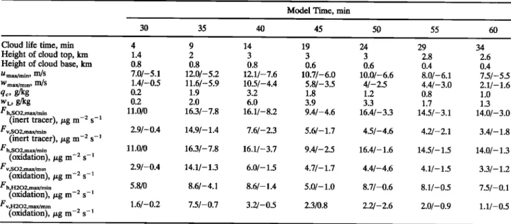
/,t max/min, m/s 7.0/-5.1 12.0/-5.2 12.1/-7.6 10.7/-6.0 10.0/-6.6 8.0/-6.1 7.5/-5.5 Wmax/mi n, m/s 1.4/-0.5 11.6/-5.9 10.5/-4.4 5.8/-3.5 4/-2.5 4.4/-3.0 2.1/- 1.6 qc, g/kg 0.2 1.9 3.2 1.8 1.2 0.8 1.0 w L, g/kg 0.2 2.0 6.0 3.9 3.3 1.7 1.3 Fh,sO2,max/min 11.0/0 16.3/-7.8 16.1/-8.2 9.4/-4.6 16.4/-3.3 14.5/-3.1 14.0/-3.0 (inert tracer),/xg m -2 s -] Fv, so2,max/min 2.9/-0.4 14.9/- 1.4 7.6/-2.3 5.6/- 1.7 4.5/-4.6 4.2/-2.1 3.4/- 1.8 (inert tracer), txg m -2 s -] Fh,sO2,max/min 11.0/0 16.3/-7.8 16.1/-3.7 9.4/-2.5 16.4/- 1.6 14.5/- 1.5 14.0/- 1.3 (oxidation),/xg m -2 s -] Fv, so2,max/min 2.9/-0.4 14.1/- 1.3 6.0/- 1.5 4.7/- 1.7 4.4/-4.6 4.1/- 1.5 3.3/- 1.2 (oxidation),/xg m -2 s -] Fh,H202,max/min 5.8/0 8.6/-4.1 8.6/- 1.4 5.0/- 1.0 8.7/-0.6 8.1/-0.5 7.5/-0.1 (oxidation),/xg m -2 s -] Fv,H202,max/min 1.6/-0.2 7.5/-0.7 3.2/-0.5 2.3/0.8 2.2/- 2.6 2.0/-0.9 1.1/-0.5 (oxidation),/xg m -2 s -]
creased (see Table 1) and the precipitation has almost ceased [Flossmann, 1991 ].
Figure 2b shows the transport through cloud top where we
can see that the mass transport of the gases through cloud top
is a factor of 5-10 smaller than the transport through cloud base. This is caused by the fact that the vertical velocity at
cloud top is generally small (see Figures 3c and 4c). Until 42
min, this transport is zero. Then we note a small net loss due to an updraft at cloud top. After this, we have a net gain of
mass due to a coexistence of weak updraft and downdraft
regions at cloud top (Figures 3c and 4c) whereby the down-
drafts compensate the updrafts and reentrain previously de-
trained gas. We also note the presence of gas above cloud top
in Figures 5 and 6 which give the gas concentrations at 45 and
55 min. There we also see the strong influence of the uptake of
4.- 0. 2. 4. 6. 8. 10. 12. 14. 16. 18. 20. x(km) 0. 2. 4. 6. 8. 10. 12. 14. 16. 18. 20. x (km) 4.- 3.- 2ø- 0. 2. 4. 6. 8. 10. 12. 14. 16. 18. 20. x (km)
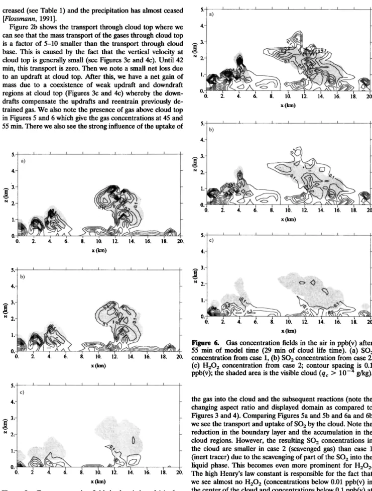
Figure 5. Gas concentration fields in the air in ppb(v) after
45 min of model time (19 min of cloud life time). (a) SO2
concentration from case 1, (b) SO2 concentration from case 2,
(c) H202 concentration from case 2; contour spacing is 0.1
ppb(v);
the shaded
area is the visible
cloud
(qc > 10 -4 g/kg).
4'
1
a)
0', , , , , , , , , , •
0. 2. 4. 6. 8. 10. 12. 14. 16. 18. 20. x(km) 0 • O. 2. 4. 6. g. 10. 12. 14. 16. 18 20. x (km)5. C) I
I
I
I
I
I
I
I
I
4.o.
!
,
0. 2. 4. 6. 8. 10. 12. 14. 16. 18. 20. x(km)Figure 6. Gas concentration fields in the air in ppb(v) after
55 min of model time (29 min of cloud life time). (a) SO2
concentration from case 1, (b) SO2 concentration from case 2,
(c) H202 concentration from case 2; contour spacing is 0.1
ppb(v);
the shaded
area is the visible
cloud
(qc > 10-4 g/kg).
the gas into the cloud and the subsequent reactions (note the
changing aspect ratio and displayed domain as compared to Figures 3 and 4). Comparing Figures 5a and 5b and 6a and 6b we see the transport and uptake of SO2 by the cloud. Note the
reduction in the boundary layer and the accumulation in the
cloud regions. However, the resulting SO2 concentrations in
the cloud are smaller in case 2 (scavenged gas) than case 1
(inert tracer) due to the scavenging of part of the SO2 into the
liquid phase. This becomes even more prominent for H20 2.
The high Henry's law constant is responsible for the fact that
we see almost no H202 (concentrations below 0.01 ppb(v) in
the center of the cloud and concentrations below 0.1 ppb(v) at
the edges) above i km. We find this effect also in the curves for the net mass transport (Figure 7). For the transport through cloud base (Figure 2a) we still see roughly a factor of 2-3 between H202 and S02 maintained. The transport through
18,646 FLOSSMANN AND WOBROCK: TRANSPORT OF GASES IN CONVECTIVE CLOUDS 14 12 E) 10 m 4 25
S0
2 (inert
tracer) S0
2 (oxidation)
t
H20
2
(oxidation)
cloud
boundary
t 20
// -
t,//I
_
/ -///
II .•../"
•'•....• " •
...
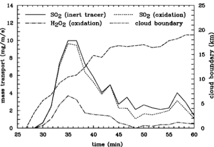
, ,,/, .•", ... • ... •'•_,•'w-•'•'•; .... 0 30 35 40 45 50 55 60 15 ••o •
o 5 time (min)Figure 7. Net transport of mass in mg m -1 s -1 into the
cloud. The long-dashed line gives the length of the cloud
boundary through which the transport occurred.
is mainly determined by the mass transport through cloud base
(compare Figure 2a) as the transports through the sides and the top are generally much smaller and often compensate each
other.
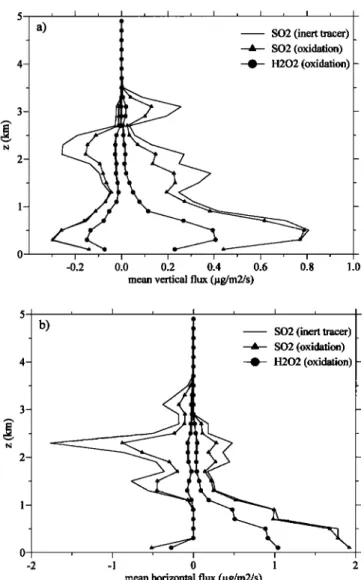
Figures 8 and 9 present a summary of the mass fluxes for 45
and 55 min as a function of height. Figures 8 and 9 are given to support later developments of parameterizations of the pro- cess of cloud venting for larger-scale models. Thus the positive and negative components of the fluxes were averaged sepa-
rately and are displayed as separate curves. Again, we see that
the qualitative behavior of all three gases is similar and only
determined by their different solubility.
Looking at Figure 8a we see that the mean vertical fluxes for
SO2 show a maximum shortly above cloud base, coupled to the maximum in vertical velocity (Figure 3c). The maximum for
H202 is much smaller and shifted toward cloud base due to its
high solubility. The maximum mean downward flux for SO2 is
found near cloud top, while for H202 the maximum mean
cloud top (Figure 2b), however, differs by roughly a factor of 8 as almost no H202 is found at cloud top.
Figures 2c and 2d give the transport through the two lateral
boundaries of the cloud which can be artificially identified in a
2-D simulation. In a simulation with no mesoscale horizontal
wind, these two transports would be identical. In the present
simulation, however, we have initialized the model with an
observed southerly flow for the horizontal wind (from left to
right in Figures 3-6 displayed by a solid line in Figures 3d and
4d) in the lower 2 km and a northerly flow in the upper part of
the atmosphere. These flows were identified with some larger-
scale clusters around the small cell under consideration
[Warner et al., 1979]. The flow is disturbed by circulations associated with this cloud which tends to develop two "rotors"
(see, e.g., Figures 3c and 3d). The strength of the resulting
horizontal fluxes depends on whether the horizontal flow of the cloud itself is in the same direction as the mesoscale flow
or opposing it. Figure 2c shows the transport through the left
boundary of the cloud. We see here in general an inflow, i.e.,
a positive contribution until 42 min, resulting from the advec-
tion with the mesoscale flow. From 42 to 47 min the outflow
part of the "cloud rotor" (see Figure 3b) dominates the trans-
port as the cloud now extends well into the inversion with the
northerly flow aloft (Figure 3d). After 45 min, the circulation
of the cell decreases
(see
Table 1) due to its decay.
Further-
more, after 50 min, the cloud top begins to subside, and con-
sequently, that part of the cloud which extends into the north-
erly flow region decreases. Thus the inflow transport again
dominates the outflow, and we have a net gain of mass. The
transport through the right cloud boundary is smaller and always represents a net loss for the cloud as the horizontal flow
field developed by the cloud at this side is acting all the time
counteracting the large-scale flow (Figures 3d and 4d). As seen
in Figures 3b and 4b, almost no gain results from the inflow in
the lowest kilometer as the horizontal inflow against the large-
scale flow is not sufficiently developed. We only see an outflow
portion which is sufficiently strong because it is mainly located in the region between 1 and 2 km and thus goes in the same direction as the large-scale flow. It is responsible for the net loss of mass through the right cloud boundary. Above, the transport again is negligible. Combining the mass transport
through all four boundaries, we can calculate a net budget for
the cloud, displayed in Figure 7. We see here that the budget
I 4- 3 2- 1- 0 . -0.6 I I I I I • I , I ,
SO2 (inert tracer)
-•- SO2 (oxidation)
• H202 (oxidation)
-d.4'-0•.2 010 012 0.4 016 018 110
mean vertical flux (l•g/m2/s)
5 I i I i
SO2 (inert tracer)
--•- SO2 (oxidation)
• H202 (oxidation)
- 0 1 2 3 4 5
mean horizontal flux (l•g/m2/s)
Figure 8. (a) Mean vertical flux and (b) horizontal flux in
m -2 s
-1 after
45 min of model
time (19 min of cloud
life time)
for the three gases considered. In Figure 8a, positive lines
represent upgoing fluxes and negative lines downgoing fluxes.
In Figure 8b, positive lines represent southerly fluxes (going to
the right in Figures 3b and 4b), and negative lines represent
downward flux is located below cloud base, again due to the
high solubility of H202 in the cloud; 10 min later, at 55 min we
see (Figure 9a) that the pattern for the vertical distribution of
the mean fluxes has changed. In addition to a maximum below
cloud base the upgoing mean vertical flux also shows a distinct
maximum above cloud top, again correlated with the field of
the vertical velocity (Figure 4c). In contrast to that, the down-
going mean flux shows its maximum inside the cloud.
The vertical distributions of the mean horizontal fluxes dis-
played in Figures 8b and 9b restate the observations made in
Figures 2-4. We see that the strongest positive mean fluxes,
representing a southerly flow, are found near the surface below
cloud base as they are embedded into the southerly large-scale
flow. The same applies to the negative mean fluxes, represent-
ing a northerly flow which is strongest between 2 km altitude
and cloud top.
The total masses associated with the transport through the
four different cloud boundaries and the net transport are given
a)
so2
(inert
tracer)
--•-- SO2 (oxidation)
4 -•- H202 (oxidation)
' -0.2 ' 0.0
0.2
0.4
0.6
0.8
1.0
mean vertical flux (gg/m2/s)
b)
t
-- SO2
(inert
tracer)
•
--•-- SO2
(oxidation)
i
1
I
-2 - 0 1 2
mean horizontal flux ([tg/m2/s)
Figure 9. (a) Mean vertical flux and (b) horizontal flux in gg m -2 s -x after 55 min of model time (29 min of cloud life time)
for the three gases considered. In Figure 9a, positive lines
represent upgoing fluxes, and negative lines represent down-
going fluxes. In Figure 9b, positive lines represent southerly fluxes (going to the right in Figures 3b and 4b), and negative
lines represent northerly fluxes (going to the left in Figures 3b
and 4b).
Table 2. Total Masses Transported Through the 2-D Boundaries
SO 2 SO 2 H202
(Inert Tracer) (Oxidation) (Oxidation)
total g/m 7.4 6.8 2.3 cloud base• total g/m 1.0 0.6 0.1 cloud top• total g/m 0.7 0.8 0.4 left boundary• tOtal g/m - 1.3 - 1.3 -0.7 right boundary• T tøtal (2-D), g/m 7.8 6.9 2.1
in Table 2. These variables pertain to a 2-D cloud with unit depth. Considering an average cloud base length of 5 km as
explained in the section on analysis of the data (dimensions
during the most active period, compare to Figure 2a), we can estimate from Table 2 the total mass transfer of a 3-D cloud
from the boundary layer to the free troposphere to be 37 kg for
SO2 as an inert tracer, 34 kg for SO2 as a scavenged species,
and 12 kg for H202. This corresponds to roughly 60% of the
pollutant mass initially present in the boundary layer (this
number depends on the size of the computational domain).
However, not all this material will be found at a given time in
the atmosphere. This will only apply to the case of the inert
tracer. SO2 will be taken up into the cloud where it will be oxidized and transported to the surface with precipitation.
Consequently, the fraction remaining in the atmosphere will
vary but generally ranges around 75%. As H202 has a much higher solubility, only about 30% of the material transported upward will actually be found in the atmosphere. The rest is
scavenged rather efficiently by the cloud drops, whereby the
scavenging is almost complete in the center of the cloud. Gas-
eous H20 2 can only be found at the cloud edges where the liquid water content is rather small.
Summary and Conclusions
We have used the DESCAM model in a 2-D dynamic frame-
work. Assuming a local pollution layer of SO2 and H202 due to
emission at the ground and an even mixture in a marine bound-
ary layer of 400 m, we have calculated the vertical and hori-
zontal redistribution of these gases caused by a warm convec-
tive cloud. In order to cover the different solubilities of
atmospheric gases we have performed two case studies. In the
first case we have used SO2 as an inert tracer by artificially
suppressing any uptake by the cloud drops. Even though this is
an unrealistic scenario, it is nevertheless useful. First, as SO2 is
not interacting with the cloud, it can be considered as a generic
inert tracer so the results obtained would apply to any inert gas with similar distribution, taking into account the differences in molecular weight. Second, case 1 serves as a control for a
comparison with the second case study where SO2 and H202
are scavenged by the cloud drops. In the cloud, S(4) is oxidized
to S(6) with the help of H202 and 03 which are simultaneously
present. The comparison between SO2 from case 1 (inert
tracer) and case 2 (scavenged gas) gives information on the
contribution of cloud chemistry to the process of cloud venting.
Studying the vertical fluxes of the gases in the two cases, as well as the mass transport and the development of the vertical
distribution of the gases, we can draw the following conclusions:
1. An inert tracer is depleted from the boundary layer and
transported upward by a convective cloud. For the medium-
18,648 FLOSSMANN AND WOBROCK: TRANSPORT OF GASES IN CONVECTIVE CLOUDS
through
cloud
base
(initial MBL concentration
of 1.4/a,g/m
3)
corresponding to 60% of the initial pollutant mass in the MBL
surrounding the cloud. Both the upward and downward fluxes
at cloud top are at least a factor of 5 smaller than the inflow at
cloud base. The transport through the sides is strongly influ-
enced by the ambient mesoscale flow influencing cloud circu-
lation.
2. The results showed little sensitivity to either using SO2
as an inert tracer or as a gas scavenged and oxidized by the
cloud drops. The mass of SO2 transported through the cloud
boundaries differs only marginally at cloud base. However, at cloud top the two cases differ by a factor of 2, which reflects the integrated history of the SO2 uptake by the cloud. The total
mass transport across cloud base introduces 34 kg of SO2 into
the free troposphere which corresponds again to 60% of the
SO2 mass initially present in the surrounding MBL. Owing to
the uptake into the cloud drops, however, after half an hour of
cloud life time only about 75% of the gas is actually in the air ready to participate in long range transport if the cloud would
suddenly disappear. Part of the scavenged SO2 is present as
S(6) in the cloud drops and part as S(4) which could eventually
desorb again. Of this scavenged SO2 a certain fraction has
already left the atmosphere because it has been redistributed
through collision and coalescence into the large drops which
have dropped to the surface as precipitation [cf. Flossmann,
1994].
3. As an example of a highly soluble gas, H202 was con-
sidered. Taking into account the fact that 0.5 ppb H202 results
in a factor of 2 lower mass concentration than SO2 (MBL
concentration 0.76/a,g/m3), the mass transport of H202 across
cloud base has the same magnitude as for SO2. Actually, about 12 kg (60% of the mass initially present in the surrounding
MBL) were transported out of the boundary layer through a
cloud base of roughly 25 km 2 as compared to 34 kg for SO2.
The fluxes through the other boundaries are rather small as
almost all H202 (70%) was scavenged by the cloud drops and
partly used up during the sulfur oxidation process.
4. The vertical distribution of the mean horizontal and
vertical fluxes was studied. Here it was found that in general
the vertical fluxes are strongest near cloud base and cloud top
displaying a clear minimum in the middle of the cloud. The
mean horizontal fluxes, however, are mainly determined by the
ambient mesoscale flow.
A major shortcoming of this work is that the model in its
present configuration is two-dimensional. Consequently, the
estimates for 3-D clouds are simply extrapolations giving just
the order of magnitude of the transport. We are presently
working on an extension of the model to three dimensions.
These results presented pertain to a medium-sized cumulus
cloud in the ITCZ. However, similar profiles of temperature and moisture are also found in larger areas of the subtropical and tropical oceans [Garret, 1992; Cotton and Anthes, 1989]. They also show a well-mixed layer at the surface of 400 to 600 m in depth and a weakly mixed layer above where the cloud forms. The cloud layer is then topped by the very dry and
persistent trade wind inversion which will be found at a similar
altitude to the transient inversion of GATE day 261. Conse-
quently, the results obtained here can be applied to a very wide
range of medium-sized cumuli and a rather large area. Even though the exchange in higher altitudes is limited in these latitudinal regions due to the persistent trade wind inversion,
we can nevertheless speculate that through entering the trade
winds the pollutants will be transported over much wider dis-
tances than in the low mixed layer. Eventually, they might
enter the ITCZ and be transported by the deep convection to
even higher altitudes, emphasizing the climatic relevance of
the cloud venting even by rather small clouds.
Acknowledgments. The authors acknowledge with gratitude the support by the European Community under EV5V-CT93-0313. They are solely responsible for the content of this manuscript. The authors thank William D. Hall for his support in installing the new version of the dynamical code and William R. Cotton for this help to improve the manuscript. The calculations for this paper have been done on the Cray C98 and C94 of the "Institut du D6veloppement et des Res- sources en Informatique Scientifique" (IDRIS, CNRS) in Orsay (France) under project 940180. The authors acknowledge with grati- tude the hours of computer time and the support provided. Further- more, the authors acknowledge the support provided by the French national program PATOM.
References
Briimmer, B., Mass and energy budgets of a 1 km high atmospheric box over the GATE C-scale triangle during undisturbed and disturbed
weather conditions. J. Atmos. Sci., 35, 997-1011, 1978.
Chatfield, R. B., and P. J. Crutzen, Sufur dioxide in remote oceanic air: Cloud transport of reactive precursors, J. Geophys. Res., 89, 7111-
7132, 1984.
Ching, J., The role of convective clouds in venting ozone from the mixed layer, paper presented at 3rd Joint Conference on Applica- tion of Air Pollution Meteorology, Am. Meteorol. Soc., San Anto-
nio, Tex., Jan. 12-15, 1982.
Clark, T. L., A small scale dynamic model using terrain-following coordinate transformation, J. Cornput. Phys., 24, 186-215, 1977. Clark, T. L., Numerical simulations with a three dimensional cloud
model, J. Atmos. Sci., 36, 2191-2215, 1979.
Clark, T. L., and R. D. Farley, Severe downslope windstorm calcula- tions in two and three spatial dimensions using anelastic interactive grid nesting, J. Atmos. Sci., 41,329-350, 1984.
Clark, T. L., and R. Gall, Three dimensional numerical model simu-
lations of air flow over mountainous terrain: A comparison with
observation, Mon. Weather Rev., 110, 766-791, 1982.
Cotton, W. R., and R. A. Anthes, Storm and Cloud Dynamics, 883 pp., Academic, San Diego, Calif., 1989.
Cotton, W. R., G. D. Alexander, R. Hertenstein, R. L. Walko, R. L.
McAnelly, and M. Nicholls, Cloud venting--A review and some new global annual estimates, Earth Sci. Rev., 39, 169-206, 1995. Cuong, N. B., B. Bonsang, and G. Lambert, The atmospheric concen-
tration of sulfur dioxide and sulfate aerosols over Antarctic, Sub-
antarctic areas and oceans, Tellus, 26, 241-249, 1974.
Emanuel, K. A., Atmospheric Convection, 580 pp., Oxford Univ. Press,
New York, 1994.
Ferek, R. J., R. B. Chatfield, and M. O. Andreae, Vertical distribution of dimethylsulfide in the marine atmosphere: Implications for the atmospheric sulfur cycle, Nature, 320, 514-516, 1986.
Flossmann, A. I., The scavenging of two different types of marine aerosol particles using a two-dimensional detailed cloud model, Tel- lus, Ser. B, 43, 301-321, 1991.
Flossmann, A. I., The effect of the impaction scavenging efficiency on the wet deposition by a convective warm cloud, Tellus, Ser. B, 45,
34-39, 1993.
Flossmann, A. I., A 2-D spectral model simulation of the scavenging of gaseous and particulate sulfate by a warm marine cloud, J. Atmos.
Res., 32, 255-268, 1994.
Flossmann, A. I., and H. R. Pruppacher, A theoretical study of the wet removal of atmospheric pollutants, part III, J. Atmos. Sci., 45, 1857-
1871, 1988.
Flossmann, A. I., W. D. Hall, and H. R. Pruppacher, A theoretical study of the wet removal of atmospheric pollutants, part I, J. Atmos.
Sci., 42, 582-606, 1985.
Flossmann, A. I., H. R. Pruppacher, and J. H. Topalian, A theoretical study of the wet removal of atmospheric pollutants, part II, J. Atmos.
Sci., 44, 2912-2923, 1987.
Garrat, J. R., The Atmospheric Boundary Layer, 316 pp., Cambridge
Univ. Press, New York, 1992.
dynamic framework: Model description and preliminary results, J. Atmos. Res., 37, 2486-2507, 1980.
Kok, G. L., Measurements of hydrogen peroxide in rainwater, Atmos. Environ., 14, 653-656, 1980.
Lelieveld, J., and P. J. Crutzen, Role of deep cloud convection in the ozone budget of the troposphere, Science, 264, 1759-1761, 1994. Lilly, D. K., On the numerical simulation of buoyant convection, Tel-
lus, 14, 148-172, 1962.
Nicholls, S., and M. A. LeMone, The fair weather boundary layer in GATE: The relationship of subcloud fluxes and structure to the
distribution and enhancement of cumulus clouds, J. Atmos. Sci., 37, 2051-2067, 1980.
Seinfeld, J. H., Atmospheric Chemistry and Physics of Air Pollution, 738 pp., John Wiley, New York, 1986.
Smagorinsky, J., General circulation experiments with primitive equa- tions, 1, Basic experiment, Mon. Weather Rev., 91, 99-164, 1963. Warner, C., J. Simpson, D. W. Martin, D. Suchman, F. R. Mosher, and
R. F. Reinking, Shallow convection on day 261 of GATE: Mesoscale arcs, Mon. Weather Rev., 107, 1617-1635, 1979.
Winklet, Surface ozone over the Atlantic Ocean, J. Atmos. Chem., 7,
73-91, 1988.
Wolff, G. T., M. S. Ruthkosky, D. P. Stroup, P. E. Korsog, M. A. Ferman, G. J. Wendel, and D. H. Stedman, Measurements of SOx, NO x and aerosol species on Bermuda, Atmos. Environ., 20, 1229-
1239, 1986.
A. I. Flossmann and W. Wobrock, Laboratoire de M•tfiorologie Physique, Universitfi Blaise Pascal, CNRS, OPGC, 24 avenue des Lan- dais, F-63177 Aubi•re Cedex, France. (e-mail: [email protected] bpclermont.fr; [email protected])
(Received August 22, 1995; revised May 6, 1996; accepted May 10, 1996.)