Intercomparison between Lagrangian and Eulerian simulations of the development of mid-latitude streamers as observed by CRISTA

HAL Id: hal-00295584

https://hal.archives-ouvertes.fr/hal-00295584

Submitted on 20 Jan 2005

HAL is a multi-disciplinary open access

archive for the deposit and dissemination of

sci-entific research documents, whether they are

pub-lished or not. The documents may come from

teaching and research institutions in France or

abroad, or from public or private research centers.

L’archive ouverte pluridisciplinaire HAL, est

destinée au dépôt et à la diffusion de documents

scientifiques de niveau recherche, publiés ou non,

émanant des établissements d’enseignement et de

recherche français ou étrangers, des laboratoires

publics ou privés.

simulations of the development of mid-latitude

streamers as observed by CRISTA

F. Khosrawi, J.-U. Grooß, R. Müller, P. Konopka, W. Kouker, R. Ruhnke, T.

Reddmann, M. Riese

To cite this version:

F. Khosrawi, J.-U. Grooß, R. Müller, P. Konopka, W. Kouker, et al.. Intercomparison between

Lagrangian and Eulerian simulations of the development of mid-latitude streamers as observed by

CRISTA. Atmospheric Chemistry and Physics, European Geosciences Union, 2005, 5 (1), pp.85-95.

�hal-00295584�

SRef-ID: 1680-7324/acp/2005-5-85 European Geosciences Union

Chemistry

and Physics

Intercomparison between Lagrangian and Eulerian simulations of

the development of mid-latitude streamers as observed by CRISTA

1_{Institut f¨ur Chemie und Dynamik der Geosph¨are I: Stratosph¨are (ICG-I), Forschungszentrum J¨ulich, 52425 J¨ulich, Germany} 2_{Institut f¨ur Meteorologie und Klimaforschung, Forschungszentrum Karlsruhe, 76344 Eggenstein-Leopoldshafen, Germany} 3_{now at: Department of Meteorology, Stockholm University, 106 91 Stockholm, Sweden}

Received: 1 July 2004 – Published in Atmos. Chem. Phys. Discuss.: 5 October 2004 Revised: 10 January 2005 – Accepted: 13 January 2005 – Published: 20 January 2005

Abstract. During the CRISTA-1 mission three pronounced

fingerlike structures reaching from the lower latitudes to the mid-latitudes, so-called streamers, were observed in the mea-surements of several trace gases in early November 1994. A simulation of these streamers in previous studies employing the KASIMA (Karlsruhe Simulation Model of the Middle Atmosphere) and ROSE (Research on Ozone in the Strato-sphere and its Evolution) model, both being Eulerian mod-els, show that their formation is due to adiabatic transport processes. Here, the impact of mixing on the development of these streamers is investigated. These streamers were simu-lated with the CLaMS model (Chemical Lagrangian Model of the Stratosphere), a Lagrangian model, using N2O as long-lived tracer. Using several different initialisations the results were compared to the KASIMA simulations and CRISTA (Cryogenic Infrared Spectrometer and Telescope for the At-mosphere) observations. Further, since the KASIMA model was employed to derive a 9-year climatology, the quality of the reproduction of streamers from such a study was tested by the comparison of the KASIMA results with CLaMS and CRISTA. The streamers are reproduced well for the North-ern Hemisphere in the simulations of CLaMS and KASIMA for the 6 November 1994. However, in the CLaMS sim-ulation a stronger filamentation is found while larger dis-crepancies between KASIMA and CRISTA were found es-pecially for the Southern Hemisphere. Further, compared to the CRISTA observations the mixing ratios of N2O are in general underestimated in the KASIMA simulations. An im-provement of the simulations with KASIMA was obtained for a simulation time according to the length of the CLaMS simulation. To quantify the differences between the simu-lations with CLaMS and KASIMA, and the CRISTA obser-vations, the probability density function technique (PDF) is used to interpret the tracer distributions. While in the PDF of

Correspondence to: F. Khosrawi

(f.khosrawi@fz-juelich.de)

the KASIMA simulation the small scale structures observed by CRISTA are smoothed out due to the numerical diffusion in the model, the PDFs derived from CRISTA observations can be reproduced by CLaMS by optimising the mixing pa-rameterisation. Further, this procedure gives information on small-scale variabilities not resolved by the CRISTA obser-vations.

1 Introduction

While the transport of air masses from the troposphere into the stratosphere occurs mainly in the tropics (Holton et al., 1995) the exchange in the stratosphere between the mid-latitudes and the tropics is hindered by a subtropical transport barrier (e.g. Trepte et al., 1993; Plumb, 1996). However, ob-servations of long-lived chemical compounds and analyses of conserved meteorological quantities such as Ertel’s potential vorticity (Ertel, 1942) indicate that some transport between the mid-latitudes and the tropics does occur in the form of so-called streamers (e.g. Waugh, 1993; Randel et al., 1993). These streamers are pronounced fingerlike structures which reach from the lower latitudes into the mid-latitudes. Stream-ers have been identified at all altitudes from the tropopause to the middle stratosphere. Waugh (1993, 1996) showed that these streamers are linked to disturbances of the po-lar vortex caused by planetary wave activity. A rather pro-nounced streamer caused by large planetary-wave activity and the associated vortex displacement was observed during the CRISTA-2 mission in the Southern Hemisphere (Riese et al., 2002).

The CRISTA instrument was flown first during the CRISTA-1 mission on board the Space Shuttle from 4 to 12 November 1994 (Offermann et al., 1999; Riese et al., 1999a). During the CRISTA-1 mission in early November 1994 three streamers were observed (Offermann et al., 1999; Riese et al., 1999b). Two of the observed streamers were located in

the Northern Hemisphere while the third was located in the Southern Hemisphere. The three pronounced streamers ob-served by the CRISTA experiment on 6 November 1994 were simulated previously by Riese et al. (1999b) and Kouker et al. (1999) employing Eulerian models, the ROSE and the KASIMA model, respectively. Eyring et al. (2003) em-ployed the KASIMA model nudged with ECMWF analyses in T42 resolution and the coupled chemistry-climate model ECHAM4.L39(DLR)/CHEM (E39/C) to establish streamer climatologies. They derived a 9-year climatology (1990-1998) with each of both models by counting all streamer events between 21 and 25 km. By comparing the streamer climatologies derived with the KASIMA model and the E39/C model they showed that both climatologies were qual-itatively in agreement and that in both models the highest streamer frequencies occurred in the Northern Hemisphere in winter. The aim of the study by Eyring et al. (2003) was to use the KASIMA model, driven by ECMWF meteorological analysis, as a reference to check the abilities and deficiencies of E39/C with respect to the temporal and spatial distribution of streamers in the model.

Here, we employ the CLaMS model (McKenna et al., 2002a,b) to test the quality of reproduction of streamers in the results of the KASIMA model. This is done in the frame of a specific case study for which CRISTA observations are available to perform a model validation. Thus, we focus on the streamers observed by CRISTA in early November 1994. We compare the results of the 9-year model run and two short term sensitivity runs of KASIMA obtained for the streamers on 6 November 1994 with the results obtained with CLaMS for the same date. In this way, an intercomparison between Eulerian and Lagrangian simulations of the development of mid-latitude streamers will be given here. Further, we es-tablish a link between the pure model study of Eyring et al. (2003) and the CRISTA observations which allows to discuss to which extent the simulated streamers in the climatology are supported by observations. Finally, we calculate proba-bility density functions (PDF) of the N2O fields measured by CRISTA and simulated by the CLaMS and KASIMA model. These PDF’s are used to quantify differences between the different model types (Eulerian and Lagrangian), differences due to different model resolutions used in KASIMA (T42 and T106) and differences between the derived model fields and CRISTA measurements. However, differences between KASIMA and CLaMS are also expected due to the fact that the vertical coordinate of the two models are different.

2 Model descriptions

2.1 The Chemical Transport Model KASIMA

The KASIMA model is a global circulation model including stratospheric chemistry for the simulation of the behaviour of physical and chemical processes in the middle atmosphere

(Reddmann et al., 2001; Ruhnke et al., 1999a). The meteo-rological component is based on a spectral architecture with the pressure altitude z=−H ln(p/p0)as vertical coordinate where H =7 km is a constant atmospheric scale height, p is the pressure, and p0=1013.25 hPa is a constant reference pressure. The meteorology module of the KASIMA model consists of three versions: the diagnostic model, the prognos-tic model and the nudged model which combines the prog-nostic and diagprog-nostic model (Kouker et al., 1999).

For the simulation of the streamers observed by CRISTA on 6 November 1994 the nudged model version is used. In this version, the model is nudged towards the ECMWF re-analyses (ERA-15, until 1994) and operational analyses thereafter. A correction is solely applied to the temperature field after integrating the primitive equations in the prognos-tic model. That is, the calculated temperature is nudged to-wards the ECMWF analysed temperature using a Newtonian cooling like algorithm. The setup of the nudging coefficient is taken from the experience obtained from sensitivity stud-ies (Kouker et al., 1999). A horizontal resolution of T42 (2.8◦×2.8◦) and 63 vertical levels between 10 and 120 km altitude with a resolution of 750 m in the middle stratosphere are used. The model is initialised in 1990 with an atmo-sphere at rest and a barotropic temperature field taken from the U.S. Standard Atmosphere (1976). The model runs con-tinuously until 1998. In the KASIMA model an idealised tracer representing stratospheric N2O is transported by the model winds. The tracer has a source region in the equa-torial lower stratosphere and a loss through photolysis de-pending on altitude and solar zenith angle only (Eyring et al., 2003). The KASIMA transport algorithm is formulated as a two step flux corrected algorithm (Zalesak, 1979). A first or-der upwind scheme from Courant et al. (1962) is used which is followed by an antidiffusive step based on the difference between the scheme of Lax and Wendroff (1960) and the first order scheme multiplied by a limiter function given by Roe and Baines (1982).

2.2 The Chemical Lagrangian Model CLaMS

The CLaMS model is a chemistry transport model which simulates the dynamics and chemistry of the atmosphere along trajectories of multiple air parcels (McKenna et al., 2002a,b). Trajectories are calculated using a fourth-order Runge-Kutta scheme (Sutton et al., 1994) with a 30-min time step. Here, wind fields were taken from the United Kingdom Meteorological Office (UKMO) Stratosphere-Troposphere Data Assimilation System (Swinbank and O’Neill, 1994). The UKMO data have a meridional and zonal resolution of 2.5◦and 3.75◦, respectively. The vertical coverage is from 1000 to 0.316 hPa with 22 quasi-logarithmic levels. Analy-ses are available every day at 12:00 UT.

The mixing of different air masses, that means the inter-action between neighbouring air parcels, is introduced by both combining air parcels and adding new air parcels under

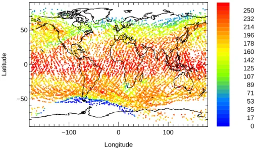
−100 0 100 Longitude −50 0 50 Latitude 0 17 35 53 71 89 107 125 142 160 178 196 214 232 250

Fig. 1. CRISTA observations of N2O between 4 November 1994, 21:00 UT and 6 November 1994, 12:00 UT at 2=675±25 K transformed to a synoptic time (6 November 12:00 UTC) by trajectory calculations.

certain conditions determined by the deformation of the flow (McKenna et al., 2002b; Konopka et al., 2003). The inten-sity of mixing is controlled by the Lyapunov exponent λ for a given spatial resolution r0 and a given mixing time step

1t. The Lyapunov exponent is a measure of the deforma-tion rate of the horizontal wind field and switches on mixing in the flow regions where λ exceeds the critical Lyapunov exponent λc, that is, in flow regions for which the

deforma-tion of the flow is strong enough (Konopka et al., 2003). The CLaMS simulations suggest a temporally and spatially inho-mogeneous mixing in the lower stratosphere with a lateral (across the wind) effective diffusion coefficient of the order of 103m2s−1. Optimised mixing parameters were deduced as an mixing time step of 1t=24 h and a critical Lyapunov exponent λc ranging between 0.8 and 1.2 d−1by Konopka

et al. (2003) from the comparison of simulations of CLaMS with spatially highly resolved ER-2 observations. However, we will show below that if coarsely resolved satellite data is considered the best results are obtained with slightly dif-ferent mixing values of λc=1.5 d−1 and 1t=12 h as

re-cently discussed in Konopka et al. (2005) for the simulation of CRISTA observations.

3 CRISTA observations

CRISTA is a limb scanning instrument which measures the thermal emission (4–71 µm) of 15 trace gases, and of aerosols and clouds. CRISTA has a high spatial resolution in all three dimensions (typically 6◦in longitude, 3◦in lati-tude and 2 km vertical). The horizontal distance of two adja-cent measurement points is about 200 km along the flight track and 650 km across the flight track. The CRISTA-1

mission was conducted from 4–12 November 1994 and the CRISTA instrument was launched aboard the NASA Space Shuttle “Atlantis” into a 300 km, 57◦_{orbit. The CRISTA}

in-strument was mounted on the CRISTA Shuttle Pallet Satellite (SPAS) platform which operates at a distance of 20–100 km behind the shuttle. Several different photochemically active gases like O3, ClONO2, HNO3, NO2, N2O5as well as the long-lived tracers CFC-11, N2O and CH4 have been mea-sured (Offermann et al., 1999; Riese et al., 1999a). Here, we focus on the CRISTA measurements of N2O. The systematic and statistical errors are 26% and 3%, respectively, at 25 km and 23% and 3.5%, respectively, at 30 km (Version 3 data). A description of the CRISTA error analysis can be found in Riese et al. (1999a).

The N2O distribution on the 675±25 K isentropic sur-face observed by CRISTA on 6 November 1994 is shown in Fig. 1. Here, asynoptic profiles observed between 4 Novem-ber and 6 NovemNovem-ber were transformed to the synoptic time on 6 November, 12:00 UTC, by using isentropic forward tra-jectories. The 675±25 K level has been chosen since at this level streamers are most pronounced. The measurements show a typical distribution with high N2O mixing ratios in the tropics and low mixing ratios towards the polar regions. The southern hemispheric polar vortex is noticeable as a re-gion with very low mixing ratios centered near 70◦W and 60◦S due to the strong descent of air masses inside the polar vortex.

At mid-latitudes, the N2O distribution exhibits three nar-row tongues (streamers) showing tropical values of N2O in the mid-latitude regions. Two of these three streamers are located in the Northern Hemisphere while the third one is lo-cated in the Southern Hemisphere. The first streamer is orig-inating at about 120◦W, 30◦N pointing northeast to about

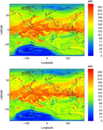
−100 0 100 Longitude −50 0 50 Latitude 0 17 35 53 71 89 107 125 142 160 178 196 214 232 250 N2O [ppbv]

Fig. 2. Result of the KASIMA 9-year run for the 6 November 1994.

0◦E, 60◦N while the second one is originating at about 90◦E, 30◦N pointing northeast to about 180◦E, 60◦N. The southern hemispheric streamer is originating at 90◦W, 20◦S pointing southeast to about 20◦E, 45◦S. Following Offer-mann et al. (1999) these three streamers will hereinafter re-ferred to as the (1) Atlantic streamer, (2) the east Asian streamer, and (3) the Southern Hemisphere streamer. The Southern Hemisphere streamer, however, is much weaker pronounced than those in the Northern Hemisphere as can be observed in the weak gradient of N2O.

4 Model simulations

4.1 Model setup of the CLaMS simulations

To obtain a meaningful comparison of the results of CLaMS and KASIMA, the CLaMS simulation was initialised with the results of the 9-year run of KASIMA (Eyring et al., 2003). That is, both model simulations start with the same initial conditions. The CLaMS simulation was initialised for 20 October and was run until 6 November 1994. The simu-lation time of 17 days should be sufficient to investigate the influence of mixing processes on the N2O distribution and on the development of streamers, since this length of simulation time is about the time scale where mixing processes become important (Konopka et al., 2005).

We also performed simulations with a shorter simulation time (8 days, not shown) initialising the CLaMS simulation on 29 October; the date used by Kouker et al. (1999) for their KASIMA simulations. In general, with both the 8-day and 17-8-day simulation, similar results were achieved. In the shorter run (8 days) the three streamers are already dis-tinguishable. However, in the longer model run (17 days) a more distinctive filamentation is found showing that the longer run is on a time scale which is more suitable for studying mixing processes as already stated in Konopka et al. (2005).

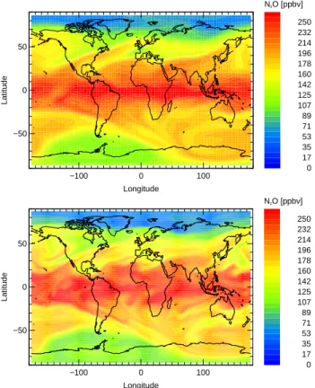
Fig. 3. CLaMS simulation with high resolution (top) and low resolution (bottom) for the 6 November 1994 (Table 1, case B). The CLaMS simulation was initialised on 20 October 1994 with KASIMA model results (2=675 K).

The CLaMS simulations were made on an isentropic level of 2=675 K negelecting diabatic effects, using UKMO data to drive the model, an mixing time step of 1t =24 h and a Lyapunov exponent of λ=1.2 (in-situ optimised mixing, (Konopka et al., 2003)). The isentropic level of 2=675 K (≈27 km) was chosen since N2O is a good dynamical tracer at this level. Further, the streamers are most pronounced at these altitudes in the CRISTA measurements (Offermann et al., 1999; Riese et al., 1999b; Kouker et al., 1999). While in the CLaMS simulation around 50 000 air parcels are used, in the KASIMA simulation only 8000 grid boxes per level are used. To allow an assessment of the impact of the spatial resolution of the model simulations to KASIMA, the simula-tion of CLaMS was repeated with a resolusimula-tion corresponding to KASIMA (approximately 8000 air parcels).

4.2 Comparison of CLaMS and KASIMA results

The results of the KASIMA (T42) model calculations de-rived for the 6 November 1994 are shown in Fig. 2 and the re-sults of the CLaMS calculation (17 days) for the same day in Fig. 3. The low resolution simulation with CLaMS (approx-imately 8000 air parcels) corresponds to the T42 simulation

Table 1. Mixing time steps and critical Lyapunov exponents used

for the CLaMS simulations initialised with KASIMA.

Case 1t, h λc, d−1 mixing intensity

A 24 2.0 reduced

B 24 1.2 in-situ optimised

C 12 1.5 satellite optimised

D 6 1.2 enhanced

of KASIMA (Fig. 3, bottom panel) while the high resolution simulation (approximately 50 000 air parcels) has a consid-erably greater spatial resolution. Both models reproduce the two northern hemispheric streamers, the Asian and the At-lantic streamer, well. However, in the CLaMS simulation the streamers are much more distinctive than in the simulation with KASIMA (Fig. 2).

The conditions in the Southern Hemisphere are not well reproduced by KASIMA. Significant differences between the KASIMA model results (Fig. 2) and the CRISTA measure-ments (Fig. 1) are evident. The location of the Southern Hemisphere streamer is not well reproduced by the KASIMA model. A possible explanation of this failure may be found in the weak pronounced features of the streamer in the CRISTA data. Small errors in KASIMA e.g. in the reproduction of the residual circulation may lead to errors in the N2O distribution in the polar vortex that in turn may affect the gradients in the streamers. This issue is known and has already been dis-cussed in detail by Kouker et al. (1999). However, an overall correctness of the residual circulation in KASIMA has been shown in Ruhnke et al. (1999b) and Reddmann et al. (2001). Further, using the low resolution model simulation of CLaMS (approximately 8000 air parcels) which is corresponding to the KASIMA resolution, the streamers are, as in the high resolution simulation, much more pronounced in the CLaMS simulation. In general, in the CLaMS simu-lation a much greater filamentation is simulated even in the simulation with the low resolution. Further, the elongated extension of the Atlantic streamer which spun up the globe measured by CRISTA is simulated in both CLaMS simula-tions, with high and low resolution, but not with KASIMA.

Both model simulations show high N2O values in the re-gion centered around 140◦W and 50◦N. This appears to be in an anticylconic circulation, which is likely part of the plan-etary wave event that caused the east Asian streamer. Further, both models show a swirling pattern centered near 120◦E and 70◦S which appears to be associated to the anticyclone that was involved in the development of the Southern Hemi-sphere streamer.

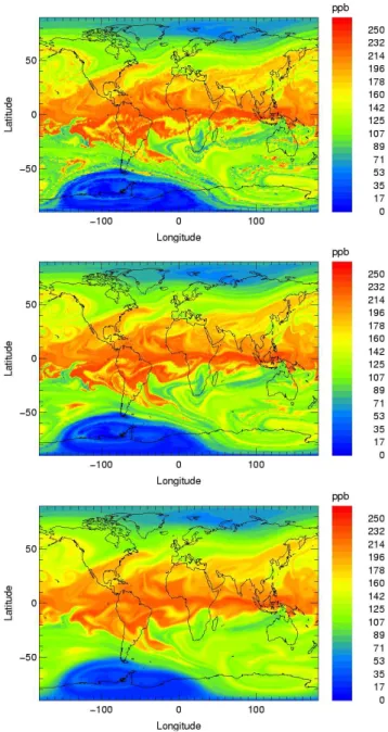
Fig. 4. CLaMS simulations with different mixing intensities for the 6 November 1994 initialised on 20 October 1994 (2=675 K) with KASIMA. Reduced mixing (top, case A), satellite optimised mixing (middle, case C) and enhanced mixing (bottom, case D).

4.3 Influence of different mixing parameterisations on the development of streamers within ClaMS

The influence of different mixing parameterisations on the filamentary structure in chemical tracer fields in CLaMS was previously investigated by Konopka et al. (2003). For a more precise estimation of the influence of the mixing parameter-isation on the formation of the streamer the CLaMS sim-ulations for the initialisation on 20 October 1994 (17 day model run, approximately 50 000 air parcels) were repeated using different mixing intensities, that is, different mixing

Table 2. Mixing time steps and critical Lyapunov exponents used

for the CLaMS simulations initialised with CRISTA.

Case 1t, h λc, d−1 mixing intensity

A 24 1.2 in-situ optimised

B 12 1.5 satellite optimised

C 6 1.2 enhanced

time steps and critical Lyapunov exponents (Konopka et al., 2003). The mixing intensity was once stronlgy reduced and once strongly enhanced. Further, we use the mixing val-ues proposed by Konopka et al. (2005) for the simulation of coarsely resolved satellite data like the CRISTA observations (Section 2.2). Thus, the following configurations of the mix-ing parameterisation are used: strongly reduced (1t=24 h,

λc=2.0 d−1), satellite optimised (1t=12 h, λc=1.2 d−1) and

strongly enhanced (1t =6 h, λc=1.2 d−1). An overview of

the employed mixing time steps and critical Lyapunov expo-nents are given in Table 1.

The simulations with different mixing time steps and Lya-punov exponents shows that the intensity of mixing in the CLaMS model has no significant influence on the forma-tion of the streamers (Fig. 4). Thus, the formaforma-tion of the streamers is primarily caused by large-scale advection of air masses out of the tropics (Riese et al., 1999b) corroborating the conclusions of the model studies by Kouker et al. (1999) and Eyring et al. (2003). However, in the Southern Hemi-sphere some differences become noticeable. For example, with increasing mixing intensity in the model, the structures are smoothed and some of the smaller filaments disappear. This is similarly observed in the Northern Hemisphere but to a somewhat smaller degree.

4.4 Comparison of the simulations with CRISTA measure-ments

The comparison of the KASIMA model results with CRISTA shows an underestimation of the KASIMA N2O values in general, especially in the Southern Hemisphere (Figs. 1 and 2). The simulated gradients in the Southern Hemisphere are too strong in the subtropics (about 20◦S) and too weak at the edge of the polar vortex. Since the CLaMS simulations were initialised with the KASIMA distribution on 20 Octo-ber these features are also found in the CLaMS result (Figs. 3 and 4). The location and the spatial extent of the Atlantic and east Asian streamer are well reproduced by KASIMA. How-ever, the location and spatial extent of the Southern Hemi-sphere streamer is not well reproduced. The differences be-tween the N2O mixing ratios simulated by KASIMA and the N2O mixing ratios measured by CRISTA are possibly due to the simplified N2O chemistry in the KASIMA model. How-ever, comparisons are limited by uncertainties of the N2O measurements of CRISTA (Riese et al., 1999a).

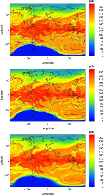
Fig. 5. CLaMS simulations with different mixing intensities for the

6 November 1994 initialised on 20 October 1994 with PV/N₂O cor-relation (2=675 K) derived from the CRISTA observations. In-situ optimised mixing (top, case B), satellite optimised mixing (middle, case C) and enhanced mixing (bottom, case D).

4.4.1 CLaMS simulation initialised with a N2O-PV corre-lation from CRISTA observations

To improve the comparison of the model results with the CRISTA observations the CLaMS model was initialised with a N2O-PV correlation which was deduced from the CRISTA data (McKenna et al., 2002a). The simulation was started on 20 October 1994 with a high spatial resolution (approx-imately 50 000 air parcels). To investigate the influence of

mixing processes on the formation of the streamer, as in the previous section, different mixing time steps and critical Lya-punov exponents were used for the simulations (Table 2): in-situ optimised mixing (1t=24 h, λc=1.2 d−1), satellite

opti-mised mixing (1t =12 h, λc=1.5 d−1) and enhanced mixing

(1t=6 h, λc=1.2 d−1).

The results of the simulation show that the simulated N2O mixing ratios are greater for this simulation than for the simulation using the results of the KASIMA 9-year run as initialisation (Fig. 5). The simulated N2O values are in good agreement with the CRISTA observations. The observed gradients in the Southern Hemisphere are well reproduced by CLaMS. Even some vortex remnants in the mid-latitudes characterised by low N2O values were reproduced. However, in the CLaMS simulation some filaments are present which were not measured by CRISTA. This may be due to the fact that the spatial resolution of the CLaMS simulation is higher than the resolution of CRISTA. CRISTA has a resolution of 200 km×650 km while in the CLaMS simulation a resolution of r0=100 km was used.

The simulations with different mixing time steps and Lya-punov exponents are not significantly different from each other. However, some differences occur in the Southern Hemisphere. Small filaments which are partly evident in the CRISTA measurement disappear due to the enhanced inten-sity of mixing (Table 2, case C). The best agreement with the CRISTA observations was achieved with an mixing time step of 1t =12 h and a Lyapunov exponent of λc=1.5 d−1

(satellite optimised case).

4.5 Impact of different meteorological analyses on CLaMS results

In the present study, KASIMA is driven by ECMWF analy-ses and CLaMS by UKMO analyanaly-ses. To investigate in how far differences in the KASIMA and CLaMS simulations are caused by differences in the employed meteorological anal-yses, we conducted CLaMS simulations driven by ECMWF (ERA-40) analyses for case B (Table 1) initialised with the results of the 9-year run of KASIMA (Fig. 6, top panel) and initialised with a N2O-PV correlation from CRISTA (Fig. 6, bottom panel). The CLaMS simulations were initialised on 20 October 1994 and were run until 6 November 1994.

The results based on ECMWF and UKMO analyses show similar structures. However, there are some differences in the details of the simulated filamentary patterns, that are partic-ularly noticeable for the Southern Hemisphere. Nonetheless, the use of different meteorological analyses is not the ma-jor cause for the differences between CLaMS and KASIMA simulations.

Fig. 6. CLaMS simulations for the 6 November 1994 driven by

ECMWF analyses to study the impact of different meteorolgical analyses on CLaMS results. The CLaMS simulations were ini-tialised on 20 October 1994. Top panel: As Fig. 3, top panel, but CLaMS driven by ECMWF analyses instead of UKMO analyses. Bottom panel: As Fig. 5, top panel, but CLaMS driven by ECMWF analyses instead of UKMO analyses.

4.6 Impact of spatial resolution and temporal coverage on KASIMA results

To assess the impact of the spatial resolution of the KASIMA model on the model results, the simulations were re-peated using a resolution of T42 and T106 (2.8◦×2.8◦ and 1.125◦×1.125◦ (250×250 km and 110×110 km), roughly corresponding to 8000 and 50.000 air parcels (with a resolu-tion of 250 km and 100 km), respectively). For these simula-tions the model was initialised with an atmosphere at rest and a barotropic temperature field taken from the U.S. Standard Atmosphere (1976) at 15 October 1994. As in the previous KASIMA simulations the nudging technique is used. The model is nudged to the ECMWF re-analyses (ERA-40, see chapter 2.1). The N2O field was initialised by an idealised tracer representing stratospheric N2O which is transported by the model winds. The tracer has a source region in the equatorial lower stratosphere (equator-wards of 15 latitude and at altitudes below 100 hPa) and a prescribed

photoly-−100 0 100 Longitude −50 0 50 Latitude 0 17 35 53 71 89 107 125 142 160 178 196 214 232 250 N2O [ppbv] −100 0 100 Longitude −50 0 50 Latitude 0 17 35 53 71 89 107 125 142 160 178 196 214 232 250 N2O [ppbv]

Fig. 7. KASIMA simulations for T42 (top) and T106 (bottom) resolution for the 6 November 1994 initialised on 15 October 1994.

sis coefficient depending on altitude and zenith angle only (Eyring et al., 2003). From many experiments it has been shown, that this combination of meteorological and chemical initialisation reveals a 3-d distribution of N2O after several days typically observed in the lower stratosphere. A simu-lation time of 20 days was used, thus allowing a three day model spin up before the 17 day simulation period for which CLaMS and KASIMA are being compared.

In general, with these KASIMA simulations a better agree-ment with the CRISTA observations was found for both the Southern and Northern Hemisphere (Fig. 7). In the Northern Hemisphere the elongated extention of the Atlantic streamer which spun up the globe is now reproduced by KASIMA. Further, the location of the Southern Hemisphere streamer is now better simulated though there is still a slight displace-ment. The absolute values of the N2O mixing ratios are better reproduced, except in the Southern Hemisphere at the loca-tion of the polar vortex where the KASIMA values are too high. In the T106 simulation more spatial structure and a stronger filamentation is found compared to the T42 simula-tion. However, some structures, like the Atlantic streamer, are smeared out.

4.7 Probability density functions (PDFs) of the observed and the simulated N2O distributions

The study of the PDFs (probability density functions) of tracer differences between APs (air parcels) separated by a prescribed distance offers an effective way to analyse the variability of tracer distributions (e.g. Sparling, 2000; Hu and Pierrehumbert, 2001, 2002). In turbulent flows, anomalously high probability of extreme spatial concentration fluctua-tions, termed “intermittency”, is expected and, consequently, the corresponding PDFs are characterised by a Gaussian core and non-Gaussian tails (e.g. Shraiman and Siggia, 2000). Konopka et al. (2005) used this technique to quantify the statistics of N2O variability both in CRISTA observations and in CLaMS simulations, and to determine the critical flow deformation and thus the critical Lyapunov exponent in CLaMS that triggers the mixing algorithm in CLaMS. Here, we apply this method in order to quantify the differences be-tween the CRISTA observations and the simulations carried out with the Eulerian model KASIMA and the Lagrangian model CLaMS.

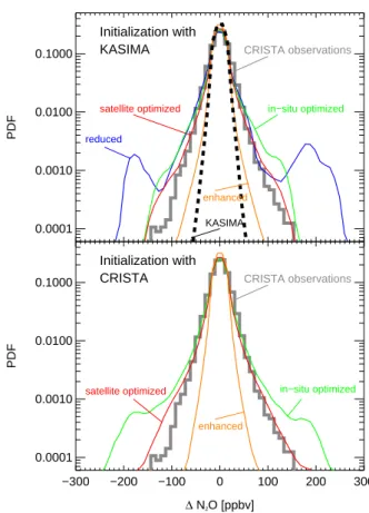
The PDFs on the 675 K isentropic surface are calcu-lated for all pairs of grid points separated by distances be-tween 100 and 300 km and, owing to the limited coverage of the CRISTA observations, with latitudes between 60◦S and 70◦N. By numbering the APs (air parcels) from north to south, only pairs with i<j are considered to avoid dou-ble counting (thus, the PDFs are not necessarily symmetric). The PDFs were calculated for the time period of the CRISTA campaign (4–12 November 1994) and the results are shown in Fig. 8, where the CLaMS PDFs are obtained from the sim-ulated N2O-distributions initialised either from the KASIMA distribution (top panel) or from the PV/N2O-correlation de-duced from CRISTA observations (bottom panel). The PDFs were also calculated for the KASIMA simulations initialised on 15 October 1994 using both a T42 and a T106 resolu-tion. However, for the KASIMA T42 simulation only 25% of the distances between the next neighbours achieved the pre-scribed distance of 100 and 300 km making thus the statistic unusable. Therefore, only the PDF for the KASIMA T106 simulation is shown in Fig. 8 (top panel). For this configura-tion, about 85% of the distances between the next neighbours vary between 100 and 300 km with lowest and highest values in the tropics and polar regions, respectively (note that this meridional bias is not present in the PDFs derived from the CLaMS distributions). In principle, the form of a PDF is not scale independent, that is it is not independent of the spatial resolution of the model in question (Hu and Pierrehumbert, 2001). However, Konopka et al. (2005), have shown (in their Fig. 6) that only a weak increase occurs in the width of the PDFs for a fourfold increase in the CLaMS model resolution. Therefore this issue can be neglected in our further discus-sion here.

The PDF derived from CRISTA observations (gray thick line in both panels of Fig. 8) is characterised by a Gaussian

core, that is most likely due to instrumental precision, and non-Gaussian tails, the so-called “fat tails”, indicat-ing an anomalously high probability of events with steep N2O gradients. These strong gradients occur mainly at the edges of the polar vortices and across streamers, filaments and vortex remnants which were sampled by CRISTA. The tails of the PDF derived from the KASIMA distributions are steeper (i.e. more Gaussian) than the CRISTA observa-tions. This indicates that numerical diffusion in the KASIMA model smoothes out the small-scale structures with strong tracer gradients observed by CRISTA.

The PDFs derived from the CLaMS simulations of the N2O-distribution strongly depend on the choice of the mix-ing parameters. The tails of these PDFs are most pro-nounced in the run with a reduced mixing intensity and are increasingly smoothed out for higher mixing intensities. The satellite optimised configuration approximates fairly well the PDF derived from CRISTA whereas the CLaMS distribu-tions obtained with the in-situ optimised and enhanced mix-ing parameterisation over- and underestimate the observed N2O variability, respectively. Even the CLaMS simulation with enhanced mixing shows slightly more pronounced PDF tails, thus, higher N2O variability than the KASIMA simula-tion. In the lower panel of Fig. 8, the same kind of sensitivity study is shown carried out for the N2O variability in CLaMS by initialising the model with CRISTA observations. The satellite optimised configuration approximates the PDF ob-tained from CRISTA better than the N2O distribution derived with in-situ optimised mixing. Further, the PDFs derived from CLaMS simulations driven by ECMWF analyses (not shown) are very similar to those derived from the CLaMS simulations driven by UKMO analyses.

As Konopka et al. (2005) argued, physical structures with scales smaller than the horizontal and vertical weighting functions of CRISTA (about 200 km and 2 km, respec-tively) are smoothed out in the observations (“optical mix-ing”). Indeed, Sparling and Bacmeister (2001) have shown that the width of PDFs derived from situ observations in-creases with the spatial resolution of the data. Therefore, the CRISTA observations may underestimate the true atmo-spheric variability of N2O, i.e. the tails in the corresponding PDFs are expected to be more pronounced in reality and may therefore better agree with the PDF obtained from the in-situ optimised simulation.

5 Conclusions

We investigated the formation and the development of the three streamers that were observed by the CRISTA-1 ex-periment on 6 November 1994. We compared the results obtained with the CLaMS model to the results of the 9-year simulation by Eyring et al. (2003) conducted with the KASIMA model. For the CLaMS simulation the N2O dis-tribution on 20 October obtained with the 9-year simulation

0.0001 0.0010 0.0100 0.1000 PDF CRISTA observations reduced

satellite optimized in−situ optimized

enhanced KASIMA Initialization with KASIMA −300 −200 −100 0 100 200 300 ∆ N2O [ppbv] 0.0001 0.0010 0.0100 0.1000 PDF CRISTA observations

satellite optimized in−situ optimized

enhanced

Initialization with CRISTA

Fig. 8. PDFs of N₂O distribution on 2=675 K observed by CRISTA (gray solid line) and calculated from the KASIMA (black dotted line) and CLaMS simulations using different mixing parameterisa-tions (enhanced mixing (orange), in-situ optimised mixing (green), satellite optimised mixing (red) and reduced mixing (blue)) for the time period of CRISTA measurements (4–12 November 1994). Top: CRISTA versus KASIMA (T106) versus CLaMS for CLaMS initialised on 20 October 1994 with KASIMA. Bottom: CRISTA versus CLaMS for CLaMS initialised with the PV/N2O-correlation deduced from CRISTA observations.

conducted with KASIMA was used as initialisation. Further, the results from both models were compared to the CRISTA observations.

The CLaMS model as well as the KASIMA model re-produces the streamers observed on 6 November 1994 well. However, a stronger filamentation than in KASIMA is present in all CLaMS simulations, both in the high resolution (approximately 50.000 air parcels) and in the low resolution (approximately 8000 air parcels) simulations. In the South-ern Hemisphere, the observed gradients in N2O are underes-timated by KASIMA. In general, the N2O values simulated by KASIMA are lower in both hemispheres than measured by CRISTA. This is possibly caused by the employed initial-isation of the 9-year run of KASIMA or by the fact that the simulation was made for a time period of 9-years and there-fore that a simplified N2O chemistry had to be implemented. However, uncertainties in the CRISTA N2O measurements have to be taken into account.

To improve the results of the CLaMS simulations we also used a N2O-PV correlation derived from CRISTA measure-ments as initialisation. For this comparison a better agree-ment between measureagree-ments and model results was obtained. In contrast to the initialisation with the KASIMA model re-sults, the N2O gradients in the Southern Hemisphere were well reproduced by CLaMS. Therefore, our results show that the initialisation used for the model simulation significantly influences the results of the simulation. Thus, an initialisa-tion based on measurements is essential for a realistic model simulation.

Further, whether an Eulerian or a Lagrangian model is more adequate for the simulation depends on the intention of the scientific studies. In case of a streamer climatology as in Eyring et al. (2003) an Eulerian model is particularly suitable since such models require much less computer effort than Lagrangian models. This is a significant advantage for long-term simulation studies over several years. In the study of Eyring et al. (2003) a streamer climatology was derived with KASIMA and compared to the ECHAM4.L39(DLR)/CHEM (E39/C) model showing a good agreement between both models. Although from a case study as the one presented here no conclusions on the validity of a climatology can be drawn, the agreement between the principle features of the CLaMS and KASIMA simulations with the streamer struc-tures observed by CRISTA gives confidence in the ability of KASIMA to simulate the large scale structure of streamers. However, if the intention is to investigate the development and fine scale structure of certain streamers a high resolution Lagrangian model, such as the CLaMS model, seems more appropriate.

However, simulations with KASIMA on a shorter time scale corresponding to that of the CLaMS simulations, and the usage of different spatial resolutions showed an improve-ment of the KASIMA results. A better agreeimprove-ment with the CRISTA measurements was found in both hemispheres. Fur-ther, an improvement of the absolute values of N2O mixing ratios was achieved.

PDFs (probability density functions) were calculated in or-der to quantify the differences in N2O variability between the CRISTA observations and the simulations carried out with the CLaMS and KASIMA model. The PDF derived from the KASIMA simulations indicates that the small scale structures observed by CRISTA are smoothed out in this model as a result of relatively high numerical diffusion. The PDFs derived from the CLaMS simulation depend strongly on the mixing parameterisation showing that the satellite op-timised configuration is in good agreement with the CRISTA observation. However, in the CRISTA observations, phys-ical structures are smoothed out due to “optphys-ical mixing”. Thus, through the PDFs additional information on atmo-spheric variability is given indicating that in-situ observa-tions are necessary to quantify the real mixing intensity of the stratosphere.

Acknowledgements. We would like to thank I. Langbein for

providing part of the KASIMA data. We thank the CRISTA team for providing their data and we thank the UK Meteorological Office (UKMO) and the European Centre for Medium-Range Weather Forecasts (ECMWF) for providing meteorological analyses. This work was supported by the “Vernetzungsfond” of the Helmholtz Gesellschaft (HGF).

Edited by: M. Dameris

References

Courant, R., Isaakson, E., and Rees, M.: On the solution of nonlin-ear hyperbolic differential equations, Comm. Pure Appl. Math, 5, 243–255, 1962.

Ertel, H.: Ein neuer hydrodynamischer Erhaltungssatz, Naturwis-senschaften, 30, 543–544, 1942.

Eyring, V., Dameris, M., Grewe, V., Langbein, I., and Kouker, W.: Climatologies of subtropical mixing derived from 3D models, Atmos. Chem. Phys, 3, 1007–1021, 2003,

SRef-ID: 1680-7324/acp/2003-3-1007.

Holton, J. R., Haynes, P., McIntyre, M. E., Douglass, A. R., Rood, R. B., and Pfister, L.: Stratosphere-troposphere exchange, Rev. of Geophys., 33, 403–439, 1995.

Hu, Y. and Pierrehumbert, R. T.:, The advection-diffusion problem for stratospheric flow. Part I: Concentration probability distribu-tion funcdistribu-tion, J. Atmos. Sci., 58, 1493–1510, 2001.

Hu, Y. and Pierrehumbert, R. T.: The advection-diffusion problem for stratospheric flow. Part II: Probability distribution function of tracer gradients, J. Atmos. Sci., 59, 2830–2845, 2002.

Konopka, P., Grooß, J. U., G¨unther, G., McKenna, D. S., M¨uller, R., Elkins, J. W., Fahey, D., Popp, P., and Stimpfle, R. M.: Weak influence of mixing on the chlorine deactivation dur-ing SOLVE/THESEO2000: Lagrangian modeldur-ing (CLaMS) ver-sus ER-2 in situ observations., J. Geophys. Res., 108, 8234, doi:10.1029/2001JD000 876, 2003.

Konopka, P., Spang, R., G¨unther, G., , M¨uller, R., McKenna, D. S., Offermann, D., and Riese, M.: How homogeneous and isotrop is stratospheric mixing?: CRISTA-1 observations versus transport studies with the Chemical Lagrangian Model of the Stratosphere (CLaMS), Q. J. R. Meteorol. Soc., in press, 2005.

Kouker, W., Offermann, D., K¨ull, V., Reddmann, T., Ruhnke, R., and Franzen, A.: Streamers observed by the CRISTA experiment and simulated in the KASIMA model, J. Geophys. Res., 104, 16 405–16 418, 1999.

Lax, P. D. and Wendroff, B.: Systems of conservation laws, Comm. Pure Appl. Math., 13, 217–237, 1960.

McKenna, D. S., Konopka, P., Grooß, J.-U., G¨unther, G., M¨uller, R., Spang, R., Offermann, D., and Orsolini, Y.: A new Chemi-cal Lagrangian Model of the Stratosphere (CLaMS): Part I For-mulation of advection and mixing, J. Geophys. Res., 107, 4309, doi:10.1029/2000JD000 114, 2002a.

McKenna, D. S., Grooß, J.-U., G¨unther, G., Konopka, P., M¨uller, R., Carver, G., and Sasano, Y.: A new Chemical Lagrangian Model of the Stratosphere (CLaMS): Part II Formulation of chemistry-scheme and initialisation, J. Geophys. Res., 107, 4265, doi:10.1029/2000JD000 113, 2002b.

Offermann, D., Grossmann, K.-U., Barthol, P., Knieling, P., Riese, M., and Trant, R.: Cryogenic Infrared Spectrometers and

Tele-scopes for the Atmosphere (CRISTA) experiment and middle atmosphere variability, J. Geophys. Res., 104, 16 311–16 325, 1999.

Plumb, R. A.: A “tropical pipe” model of stratospheric transport, J. Geophys. Res., 101, 3957–3972, 1996.

Randel, W. J., Gille, J. C., Roche, A. E., Kumer, J. B., Mergen-thaler, J. L., Waters, J. W., Fishbein, E. F., and Lahoz, W. A.: Stratospheric transport from the tropics to middle latitudes by planetary-wave mixing, Nature, 365, 533–535, 1993.

Reddmann, T., Ruhnke, R., and Kouker, W.: Three-dimensional model simulations of SF6 with mesospheric chemistry, J. Geo-phys. Res., 106, 14 525–14 537, 2001.

Riese, M., Spang, R., Preusse, P., Ern, M., Jarisch, M., Offer-mann, D., and GrossOffer-mann, K.-U.: Cryogenic infrared spectrome-ters and telescopes for the atmosphere (CRISTA) data processing and atmospheric temperature and trace gas retrieval, J. Geophys. Res., 104, 16 349–16 347, 1999a.

Riese, M., Tie, X., Brasseur, G., and Offermann, D.: Three-dimensional simulation of stratospheric trace gas distributions measured by CRISTA, J. Geophys. Res., 104, 16 419–16 435, 1999b.

Riese, M., Manney, G. L., Oberheide, J., Tie, X., and Offer-mann, D.: Stratospheric transport by planetary wave mixing as observed during CRISTA-2, J. Geophys. Res., 107, 8179, doi:10.1029/2001JD000 269, 2002.

Roe, P. L. and Baines, M. J.: Algorithms for advection and shock problems, in: Proc. of the 4th GAMM conference on numerical methods in fluid mechanics, edited by: H. Viviand, pp. 281–300, Vieweg, Braunschweig, 1982.

Ruhnke, R., Kouker, W., and Reddmann, T.: The influence of the OH + NO2+ M reaction on the NOypartitioning in the late arctic

winter 1992/1993 as studied with KASIMA, J. Geophys. Res., 104, 3755–3772, 1999a.

Ruhnke, R., Kouker, W., Reddmann, T., Berg, H., Hochschild, G., Kopp, G., Krupa, R., and Kuntz, M.: The vertical distribution of ClO at Ny- ˚Alesund during March 1997, Geophys. Res. Lett., 26, 839–842, 1999b.

Shraiman, B. and Siggia, E. D.: Scalar turbulence, Nature, 405, 639–646, 2000.

Sparling, L. C.: Statistical perspectives on stratospheric transport, Rev. Geophys., 38, 417–436, 2000.

Sparling, L. C. and Bacmeister, J. T.: Scale dependence of tracer microstructure: PDFs, intermittency and the dissipation scale, J. Geophys. Res., 28, 2823–2826, 2001.

Sutton, R. T., Maclean, H., Swinbank, R., O’Neill, A., and Taylor, F. W.: High-resolution stratospheric tracer fields estimated from satellite observations using Lagrangian trajectory calculations, J. Atmos. Sci., 51, 2995–3005, 1994.

Swinbank, R. and O’Neill, A.: A stratosphere-troposphere data as-similation system, Mon. Wea. Rev., 122, 686–702, 1994. Trepte, C., Veiga, R. E., and McCormick, M. P.: The poleward

dis-persal of Mount Pinatubo volcanic aerosol, J. Geophys. Res., 98, 18 563–18 573, 1993.

Waugh, D. W.: Subtropical stratospheric mixing linked to distur-bances in the polar vortices, Nature, 365, 535–537, 1993. Waugh, D. W.: Seasonal variation of isentropic transport out of the

tropical stratosphere, J. Geophys. Res., 101, 4007–4023, 1996. Zalesak, S. T.: Fully multidimensional flux-corrected transport