Comparison of high-latitude line-of-sight ozone column density with derived ozone fields and the effects of horizontal inhomogeneity

HAL Id: hal-00295928

https://hal.archives-ouvertes.fr/hal-00295928

Submitted on 29 May 2006

HAL is a multi-disciplinary open access

archive for the deposit and dissemination of

sci-entific research documents, whether they are

pub-lished or not. The documents may come from

teaching and research institutions in France or

abroad, or from public or private research centers.

L’archive ouverte pluridisciplinaire HAL, est

destinée au dépôt et à la diffusion de documents

scientifiques de niveau recherche, publiés ou non,

émanant des établissements d’enseignement et de

recherche français ou étrangers, des laboratoires

publics ou privés.

Comparison of high-latitude line-of-sight ozone column

density with derived ozone fields and the effects of

horizontal inhomogeneity

W. H. Swartz, J.-H. Yee, C. E. Randall, R. E. Shetter, E. V. Browell, J. F.

Burris, T. J. Mcgee, M. A. Avery

To cite this version:

W. H. Swartz, J.-H. Yee, C. E. Randall, R. E. Shetter, E. V. Browell, et al.. Comparison of

high-latitude line-of-sight ozone column density with derived ozone fields and the effects of horizontal

inho-mogeneity. Atmospheric Chemistry and Physics, European Geosciences Union, 2006, 6 (7),

pp.1843-1852. �hal-00295928�

Atmos. Chem. Phys., 6, 1843–1852, 2006 www.atmos-chem-phys.net/6/1843/2006/ © Author(s) 2006. This work is licensed under a Creative Commons License.

Atmospheric

Chemistry

and Physics

Comparison of high-latitude line-of-sight ozone column density with

derived ozone fields and the effects of horizontal inhomogeneity

W. H. Swartz1, J.-H. Yee1, C. E. Randall2, R. E. Shetter3, E. V. Browell4, J. F. Burris5, T. J. McGee5, and M. A. Avery4

1_{The Johns Hopkins University Applied Physics Laboratory, Laurel, MD, USA}

2_{Laboratory for Atmospheric and Space Physics, University of Colorado, Boulder, CO, USA} 3_{National Center for Atmospheric Research, Boulder, CO, USA}

4_{NASA Langley Research Center, Hampton, VA, USA} 5_{NASA Goddard Space Flight Center, Greenbelt, MD, USA}

Received: 29 August 2005 – Published in Atmos. Chem. Phys. Discuss.: 14 November 2005 Revised: 14 February 2006 – Accepted: 15 March 2006 – Published: 29 May 2006

Abstract. Extensive ozone measurements were made during the second SAGE III Ozone Loss and Validation Experiment (SOLVE II). We compare high-latitude line-of-sight (LOS) slant column ozone measurements from the NASA DC-8 to ozone simulated by forward integration of measurement-derived ozone fields constructed both with and without the assumption of horizontal homogeneity. The average bias and rms error of the simulations assuming homogeneity are rel-atively small (−6 and 10%, respectively) in comparison to the LOS measurements. The comparison improves signifi-cantly (−2% bias; 8% rms error) using forward integrations of three-dimensional proxy ozone fields reconstructed from potential vorticity–O3 correlations. The comparisons

pro-vide additional verification of the proxy fields and quantify the influence of large-scale ozone inhomogeneity. The spa-tial inhomogeneity of the atmosphere is a source of error in the retrieval of trace gas vertical profiles and column abun-dance from LOS measurements, as well as a complicating factor in intercomparisons that include LOS measurements at large solar zenith angles.

1 Introduction

Extensive measurements of ozone were made in the Arc-tic during the second SAGE III Ozone Loss and Valida-tion Experiment (SOLVE II) in winter 2003, including: in situ sampling, lidar and ozonesonde vertical profiles, line-of-sight (LOS) measurements (from the NASA DC-8 air-craft to the Sun), and satellite vertical profiles and column

Correspondence to: W. H. Swartz

(bill.swartz@jhuapl.edu)

measurements. To date, several comparisons of ozone mea-surements from this campaign have been made. Lait et al. (2004) used a quasi-conservative coordinate mapping tech-nique to compare sometimes spatially and temporally dis-parate lidar, ozonesonde, and Polar Ozone and Aerosol Mea-surement (POAM) III solar occultation vertical profiles. Liv-ingston et al. (2005) compared vertical column densities in-ferred from LOS solar measurements made by the Ames Airborne Tracking Sunphotometer (AATS-14) with similar measurements from the NCAR Direct beam Irradiance At-mospheric Spectrometer (DIAS) and NASA/Langley’s Gas and Aerosol Monitoring System (GAMS), as well as inte-grated column measurements retrieved by the Stratospheric Aerosol and Gas Experiment (SAGE) III, POAM III, Total Ozone Mapping Spectrometer (TOMS), and Global Ozone Monitoring Experiment (GOME) satellite instruments.

In this paper, we extend the evaluation of LOS ozone by comparison with other, complementary measurements. We shall focus on LOS ozone retrieved from DIAS solar irra-diance measurements using the multi-spectral, multi-species retrieval of Swartz et al. (2005). There are issues that com-plicate such evaluations of ozone, especially at high lati-tudes, including the effects of spatial (horizontal) inhomo-geneities of the ozone field. Global ozone, in terms of its ver-tical column density, ranges from tropical values of roughly 250 Dobson Units (DU) to a polar high of nearly 500 DU, before annual springtime ozone depletion occurs within the polar vortex, with total ozone reduced to a minimum of close to 100 DU. Hudson et al. (2003) have recently classified total ozone amounts into tropical, midlatitude, and polar meteo-rological regimes. The polar vortex itself circumscribes a transient fourth regime, driven by photochemical ozone loss. The boundaries of these regimes are constantly moving with

1844 W. H. Swartz et al.: Comparison of line-of-sight ozone, horizontal inhomogeneity the dynamics of the atmosphere. In addition, ozone varies on

small distance scales, smaller than the grid-scale of satellite retrievals and three-dimensional (3-D) models. These small-scale structures may occur because of dynamics, such as fil-aments drawn off of the polar vortex or in association with stratosphere–troposphere exchange.

For the present analysis, our goal is to compare DIAS LOS ozone to LOS simulations based on ozone profiles measured by other instruments during SOLVE II. Ideally, these other measurements would include a high-resolution, 3-D specifi-cation of the ozone field, which could be integrated along the DIAS line of sight, from the aircraft to the Sun. Al-though this is not available, ozone measurements made dur-ing SOLVE II were extensive, and it is possible to construct 3-D fields based on these ozone measurements. We will sim-ulate LOS ozone by forward integration of the ozone dataset, both with and without 3-D inhomogeneities, and compare these with the DIAS LOS measurements, which include hor-izontal inhomogeneities by definition. By taking the inho-mogeneity of the ozone field into consideration, we will be able to examine error associated with the assumption of at-mospheric homogeneity in the presence of large-scale ozone gradients associated with the polar vortex.

After describing the ozone datasets (Sect. 2) and how the LOS simulations were computed (Sect. 3), we will show how the simulations, with and without the homogeneity as-sumption, agree with the LOS measurements (Sect. 4). All-flight statistical comparisons will be presented, along with examples of how inhomogeneities affected specific flights. Implications for satellite retrievals will also be considered (Sect. 5).

2 SOLVE II measurements

The second SAGE III Ozone Loss and Validation Experi-ment, in combination with the Validation of International Satellites and study of Ozone Loss (VINTERSOL) cam-paign, operated from Kiruna, Sweden (68◦N, 20◦E) during January–February 2003. The NASA DC-8 hosted a suite of instruments, including: the FAST response OZone instru-ment (FASTOZ) measuring in situ ozone; the Differential Absorption Lidar (DIAL) and Airborne Raman Ozone, Tem-perature, and Aerosol Lidar (AROTAL) vertically profiling ozone; and DIAS and AATS-14 making solar LOS ozone measurements. Eleven science flights provided a substan-tial ozone dataset for intercomparison, validation, and eval-uation. For the present analysis, we focus on data from the 10 flights from 12 January through 2 February 2003, exclud-ing the final transit flight (note that the analysis of Swartz et al. (2005) was restricted to six flights from 19 January to 2 February, for comparison with available AATS-14 data). In addition, the satellite-based solar occultation instruments POAM III, the Halogen Occultation Experiment (HALOE), and SAGE II/III were all operational during SOLVE II. These

satellite data were combined to form near-global 3-D ozone fields that were used in the intercomparisons, as described below.

2.1 Sun-viewing line-of-sight ozone measurements The DC-8 was equipped with a number of instruments that measured the slant ozone column density from the aircraft to the Sun. For this analysis, we used measurements made by the NCAR DIAS instrument. DIAS is a scanning spectrora-diometer designed to determine the direct solar UV and vis-ible irradiance from 290 to 630 nm with roughly 1-nm reso-lution (Swartz et al., 2005), reporting complete spectra every 30 s. Swartz et al. (2005) developed a multi-species spectral-fitting technique for deriving LOS ozone from DIAS spec-tra during SOLVE II. Intercomparison with the NASA/Ames AATS-14 Sun photometer, also on board the DC-8, showed the instruments to be in excellent agreement, with mean and root-mean-square relative differences of roughly 2% (Swartz et al., 2005; Livingston et al., 2005). The DIAS LOS mea-surements are further evaluated here by comparison with LOS simulations based on the datasets described next. 2.2 Lidar vertical ozone profiles and in situ ozone

measure-ments

NASA/Langley’s DIAL lidar (Browell et al., 1998; Grant et al., 1998) measured the vertical ozone profile above and below the DC-8. At flight altitude (∼10 km), DIAL pro-files extend from near the surface to roughly 25 km, with the exception of within about 1 km of the DC-8 altitude itself, at 750-m vertical measurement resolution (data re-ported at 75-m intervals). Ozone profiles were rere-ported every minute along the flight track. NASA/Goddard’s AROTAL li-dar (Burris et al., 2002; McGee et al., 1995) reported ozone profiles with a vertical measurement resolution ranging from 500 to 3500 m, above the DC-8 from about 14 to 35 km (data reported at 150-m intervals), every ∼20 s.

Lait et al. (2004) made a very thorough intercomparison of the two lidar datasets, ozonesondes, and POAM III occul-tation profiles during SOLVE II, using a quasi-conservative coordinate mapping technique. Their analysis informed our combination of lidar data in this work (see Sect. 3.2.1). Lait et al. (2004) found that between roughly 16 and 24 km there was excellent agreement among datasets. Below 16 km, AROTAL was biased high relative to the other measure-ments; above 24 km, DIAL was biased high.

In situ ozone mixing ratio was provided by NASA/Langley’s FASTOZ instrument (http://cloud1. arc.nasa.gov/solveII/instrument files/O3.pdf) and converted to number density using flight pressure and temperature. FASTOZ is calibrated to a NIST-referenced ozone standard, providing a very accurate measurement of ozone at flight altitude.

W. H. Swartz et al.: Comparison of line-of-sight ozone, horizontal inhomogeneity 1845 2.3 Solar occultation profiles

A number of approaches have been used to reconstruct three-dimensional ozone fields from fundamentally sparse datasets. Formal data assimilation is one approach (e.g., Struthers et al., 2002). Trajectory mapping (e.g., Pierce et al., 1994) and reverse domain filling (e.g., Sutton et al., 1994) have also been used. Another approach, the quasi-conservative coordinate or PV mapping method, has been used quite effectively and efficiently in recent years in the po-lar regions (Butchart and Remsberg, 1986; Schoeberl et al., 1989; Randall et al., 2002, 2005; Lait et al., 2004). The essence of the technique rests on the premise that ozone behaves as a long-lived tracer in the stratosphere on short timescales and tends to be highly correlated with other, sim-ilarly long-lived dynamical tracers (e.g., potential vorticity) on an isentropic surface. Using PV and potential tempera-ture θ as coordinates, it is possible to reconstruct a “proxy” ozone field wherever PV and θ are known, based on a limited number of ozone observations that span a sufficient range of PV/θ values.

Using the same technique that has been used and validated by Randall et al. (2002) in the 1999/2000 Northern sphere and Randall et al. (2005) in the 2002 Southern Hemi-sphere winters, we produced daily, isentropic ozone proxy fields for the Arctic region during SOLVE II, using solar oc-cultation ozone profiles measured by POAM III, HALOE, and SAGE II/III, each providing ∼14 daily profiles in the Northern Hemisphere. The daily proxy fields cover the SOLVE II flight region and extend from roughly 12 to 60 km (above 1500 K or about 40 km, the proxy was based on PV at 1500 K), based on satellite data collected within a ±3-day window for each day of interest.

3 Line-of-sight ozone calculations

Combining the independent measurements of the ozone field from other measurement systems described above, we simu-lated LOS ozone for comparison with DIAS LOS measure-ments and interpretation (Swartz et al., 2005). We consid-ered both spatially homogeneous (horizontally uniform) and inhomogeneous ozone fields, with the latter capturing actual (large-scale) spatial gradients. This approach reveals the ef-fects of inhomogeneity on such LOS measurements. 3.1 Line-of-sight ozone simulation

The line-of-sight path was determined by the solar viewing geometry, and we used a numerical integrator to calculate the refracted light path through the atmosphere from the aircraft to the Sun. The integrator has recently been used to simu-late the LOS ozone during SOLVE II for comparison with DIAS measurements (Swartz et al., 2005). It has also been used to compute airmass factors for the conversion of LOS

to vertical ozone column density (Russell et al., 2005; Liv-ingston et al., 2005). (In these previous studies, the integrator has assumed a spatially homogeneous atmosphere.) Russell et al. (2005) have compared airmass calculations using the present integrator with other established techniques at mod-erate SZAs, and the agreement was excellent. Because our integrator accounts for the effects of atmospheric refraction, it is very powerful at large SZAs.

In addition to the LOS path itself, the integrator produces a set of geometric weights for each altitude layer the path passes through in the atmosphere between the DC-8 and the top of the atmosphere. The geometric weighting, when mul-tiplied by the ozone amount (the LOS ozone density profile through the atmosphere), yields a contribution function that, when summed, is the total LOS ozone column. At SZAs larger than 90◦, the light path passes through layers of the atmosphere below the aircraft altitude. These are duly ac-commodated by the integrator. For this analysis, the calcula-tions were performed from DC-8 altitude to 50 km, at 0.5-km resolution, for each point along the flight tracks.

3.2 Homogeneous ozone fields

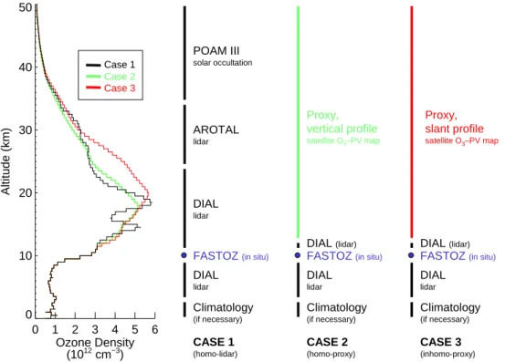
The most basic LOS ozone simulation (and the vast major-ity of satellite vertical profile retrieval algorithms) assumes spatial homogeneity of the atmosphere. The ozone field is horizontally uniform, with a particular vertical profile. In this analysis, we consider two homogeneous cases. The dif-ferent ozone profiles used for LOS simulation are summa-rized graphically in Fig. 1 and described in the following sub-sections. When computing LOS ozone in the spatially homogeneous simulations, the vertical profile was replicated over the entire line of sight, which intersects the profile at dif-ferent heights as the distance from the DC-8 increases. The LOS ozone concentration was then integrated using the ap-propriate geometric weighting function.

3.2.1 Case 1 simulation: homogeneous integration of lidar profiles

In order to calculate vertical ozone profiles for integration to simulate the DIAS observed LOS ozone, we combined a number of difference measurements. We used DIAL lidar profiles both below and above the aircraft, up to 24 km, in-terpolated to the DIAS scan times (every 30 s). In part be-cause the lidar instruments do not report data within about a kilometer above and below the DC-8 altitude, we interpo-lated the lidar profile vertically to FASTOZ in situ ozone. Because the DIAL lidar did not always reach the surface, it was desirable for the purpose of LOS simulations to estimate the ozone in the bottom few kilometers of the atmosphere (although this is only necessary at very large SZAs, when the tangent point altitude of the LOS is well below aircraft altitude). The MODTRAN radiative transfer model (Berk et al., 1989) sub-Arctic winter ozone profile was used as a

1846 W. H. Swartz et al.: Comparison of line-of-sight ozone, horizontal inhomogeneity (1012 cm−3) 0 1 2 3 4 5 6 Ozone Density 0 10 20 30 40 50 Altitude (km) POAM III solar occultation AROTAL lidar DIAL lidar DIAL lidar Climatology (if necessary) FASTOZ (in situ)

Proxy, vertical profile satellite O3–PV map Proxy, slant profile satellite O3–PV map DIAL (lidar)

FASTOZ (in situ) FASTOZ (in situ)

DIAL lidar Climatology (if necessary) DIAL lidar Climatology (if necessary) DIAL (lidar) CASE 1 (homo-lidar) CASE 2 (homo-proxy) CASE 3 (inhomo-proxy) Case 1 Case 2 Case 3

Fig. 1. Graphic representation of the three types of ozone profiles used to build the ozone fields in the simulations. Each profile was constructed by combining data from various sources from difference altitude regions at the location of the DC-8, as indicated. For Case 2, the 3-D ozone proxy field was interpolated to the DC-8 flight track to yield a vertical profile, assumed to be spatially homogeneous. In inhomogeneous Case 3, the situation is similar, except that the profile varies along the LOS, interpolated from the full three-dimensional proxy field (this variable Case-3 profile is projected onto the local vertical for the profile comparison example on the left of the figure, which is from the 26 January 2003 DC-8 flight).

climatology in this bottommost part of the profile. Above 24 km, we appended the profile with AROTAL lidar mea-surements, which extended the profile to about 35 km. The closest POAM III occultation profile extended the profile to 50 km, which was the limit of integration (an insignificant amount of ozone is above the stratosphere).

3.2.2 Case 2 simulation: homogeneous integration of proxy ozone fields

For Case 2, we first horizontally interpolated each vertical layer of the 3-D proxy field to the flight track at the DIAS scan times and then assumed a uniform atmosphere based on the interpolated vertical profile. This is directly compa-rable to the lidar profiles described above. In fact, the inter-polated proxy fields agreed closely with the combination of lidar profiles used in Case 1. Averaged over all flights, the lidar–proxy differences were <5% below 24 km and <10% above. Because the proxy field is available down to only about 12 km, we used DIAL lidar, FASTOZ in situ, and cli-matological ozone below (as in Case 1).

3.3 Case 3 simulation: inhomogeneous integration of proxy ozone fields

Case 3 integrated the full, 3-D proxy field to yield what in principle should be the most accurate, “true” LOS ozone pro-file and ozone column density. The proxy field was three-dimensionally interpolated to the LOS path, and the Case 3 “vertical” ozone profile example on the left of Fig. 1 was constructed by projecting the LOS slant profile through the 3-D proxy field onto the vertical altitude grid, for com-parison. Below the proxy (at altitudes _{.12 km), DIAL} lidar/FASTOZ/climatological profiles were used and inte-grated homogeneously (as in Cases 1 and 2).

An example of the ozone field integration is shown in Fig. 2. In the figure, the 3-D proxy has been interpolated in latitude and longitude to a particular LOS path from the 26 January 2003 flight, producing a 2-D vertical curtain oriented along the LOS, horizontally indexed to the dis-tance from the DC-8. The SZA is 90◦. The LOS path through the curtain is indicated, along with the ozone con-tribution function at each altitude layer (summed over 2.5-km bins). The contribution functions from both the inho-mogeneous (Case 3) and its difference in comparison to the homogeneous proxy (Case 2) simulations are depicted

W. H. Swartz et al.: Comparison of line-of-sight ozone, horizontal inhomogeneity 1847 1 2 3 4 5 6 Ozone Density (10 12 cm −3 ) 0 100 200 300 400 500 600 700 Range (km) 0 10 20 30 40 Altitude (km)

Fig. 2. Integration of the 3-D proxy ozone field. The 2-D curtain plot of ozone number density is oriented along the solar line of sight

(SZA=90◦, roughly to the south) with the range indicated along the

abscissa from a point along the DC-8 flight track on 26 January

2003, (71◦N, 25◦W) – the same point from which the profiles in

Fig. 1 are derived. The DC-8 was at an altitude of 11 km (indicated with a red diamond on the ordinate). Black-on-white solid circles spaced every 2.5 km in the vertical above the DC-8 indicate the path of the line of sight through the atmosphere. The areas of the solid circles are proportional to the ozone absorption contribution func-tion (ozone density × geometric weighting) in the 2.5-km layer. The white solid circles correspond to the inhomogeneous Case 3 integration of the proxy field. The black, overlying solid circles correspond to the differences between the Case 3 and homogeneous Case 2 (Case 3−Case 2) integrations of the proxy field, the latter as-suming a uniform, homogeneous field based on the vertical, 1-D in-terpolation of the proxy at the DC-8 location. The ozone total slant

column density for the Case 3 (Case 2) simulation is 2.31×1020

(2.07×1020) cm−2.

quantitatively as concentric black-on-white solid circles. The curtain plot for the corresponding uniform atmosphere (not shown) would be constant across the plot, equal to the values of the vertical profile at the DC-8. As was typical of so-lar observations during SOLVE II (viewing southward from high latitudes), ozone increases to the south along the LOS, such that the inhomogeneous simulation is larger than the corresponding homogeneous case. This is the essence of the inhomogeneity problem, resulting in a negative bias in the simulation of the homogeneous ozone field, which can be seen in both Figs. 1 and 2.

4 Comparison of LOS ozone simulations and

measure-ments

We now focus on the LOS ozone derived from DIAS mea-surements on-board the DC-8 during SOLVE II and compare this with simulations based on the homogeneous and inho-mogeneous ozone fields described above (Cases 1–3).

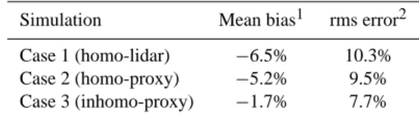
Statis-Table 1. All-flight statistical agreement between various simula-tions and DIAS line-of-sight ozone measurements.

Simulation Mean bias1 rms error2

Case 1 (homo-lidar) −6.5% 10.3%

Case 2 (homo-proxy) −5.2% 9.5%

Case 3 (inhomo-proxy) −1.7% 7.7%

1_{Mean relative difference.}

2_{Root-mean-square (rms) relative error (difference).}

tics from all of the flights considered will be shown first, fol-lowed by more detailed examples from specific flights. 4.1 All-flight comparison statistics

Because the true, 3-D ozone field is not precisely known at high spatial and temporal resolutions (and not known at all in three dimensions below the proxy field lowest alti-tude of ∼12 km), it is impossible to specifically attribute measurement–simulation discrepancies completely. But the SOLVE II dataset is sufficiently large to consider such com-parisons in the aggregate. We have examined the 10 DC-8 flights from 12 January through 2 February 2003 (exclud-ing transit flights), and the results are summarized in Table 1 (Cases 1 and 3 are also plotted in Fig. 3).

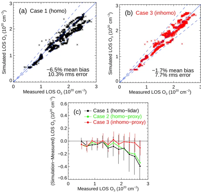
Figure 3a, based on Case 1 ozone profiles, is equivalent to the results reported by Swartz et al. (2005, Fig. 6), who noted a −9.6% mean relative (12.5% root-mean-square) difference in the simulation–DIAS measurement comparison. The rea-son for the apparent improvement in Fig. 3a is due in part to the use of AROTAL lidar data at 24–35 km, along with the addition of four more flights to the comparison (which had been restricted to six flights, for comparison with the co-manifested AATS-14 Sun photometer by Swartz et al., 2005). Case 1 simulations agree well with the LOS measurements.

The homogeneous, proxy-derived LOS ozone simulations of Case 2 provide a modest improvement in the mean bias and rms error (Table 1). This also verifies the accuracy of the ozone proxy.

Figure 3 shows the simulation–measurement improvement going from Case 1 to Case 3. The cluster of points in Fig. 3a moves closer to the 1-to-1 line in Fig. 3b, as most of the mean bias is taken into account by virtue of the ozone gradient. This improvement, Case 1-to-3 (and Case 2-to-3), gives an estimate of the effects of inhomogeneity on a LOS retrieval that assumes spatial homogeneity based on the vertical ozone profile at the DC-8 (either from lidar/in situ or the 3-D proxy interpolated to the flight track). The rms error also benefits from taking ozone inhomogeneity into account.

The absolute error associated with the homogeneity as-sumption (and size of the corresponding correction by three-dimensionally integrating the 3-D ozone field) is

1848 W. H. Swartz et al.: Comparison of line-of-sight ozone, horizontal inhomogeneity

0

1

2

3

Measured LOS O

3

(10

20

cm

−2

)

0

1

2

3

Simulated LOS O

3

(10

20

cm

−2

)

_{Case 1 (homo)}

−6.5% mean bias

10.3% rms error

(a)

0

1

2

3

Measured LOS O

₃

(10

20

cm

−2

)

0

1

2

3

Simulated LOS O

3

(10

20

cm

−2

)

_{Case 3 (inhomo)}

−1.7% mean bias

7.7% rms error

(b)

0

1

2

3

Measured LOS O

₃

(10

20

cm

−2

)

−0.6

−0.4

−0.2

0.0

0.2

0.4

0.6

(Simulation−Measured) LOS O

3

(10

20

cm

−2

)

Case 1 (homo−lidar)

Case 2 (homo−proxy)

Case 3 (inhomo−proxy)

(c)

0

1

2

3

Measured LOS O

3

(10

20

cm

−2

)

0

1

2

3

Simulated LOS O

3

(10

20

cm

−2

)

_{Case 1 (homo)}

−6.5% mean bias

10.3% rms error

(a)

0

1

2

3

Measured LOS O

₃

(10

20

cm

−2

)

0

1

2

3

Simulated LOS O

3

(10

20

cm

−2

)

_{Case 3 (inhomo)}

−1.7% mean bias

7.7% rms error

(b)

0

1

2

3

Measured LOS O

3

(10

20

cm

−2

)

−0.6

−0.4

−0.2

0.0

0.2

0.4

0.6

(Simulation−Measured) LOS O

3

(10

20

cm

−2

)

Case 1 (homo−lidar)

Case 2 (homo−proxy)

Case 3 (inhomo−proxy)

(c)

0 1 2 3 Measured LOS O3 (10 20 cm−2) 0 1 2 3 Simulated LOS O 3 (10 20 cm −2 )

_{Case 1 (homo)}

−6.5% mean bias

10.3% rms error

(a)

0 1 2 3 Measured LOS O3 (10 20 cm−2) 0 1 2 3 Simulated LOS O 3 (10 20 cm −2 )

_{Case 3 (inhomo)}

−1.7% mean bias

7.7% rms error

(b)

0 1 2 3 Measured LOS O3 (10 20 cm−2) −0.6 −0.4 −0.2 0.0 0.2 0.4 0.6 (Simulation−Measured) LOS O 3 (10 20 cm −2 )

Case 1 (homo−lidar)

Case 2 (homo−proxy)

Case 3 (inhomo−proxy)

(c)

Fig. 3. Line-of-sight ozone comparison of simulations and DIAS measurements for 10 flights during 12 January–2 February 2003: (a) homogeneous Case 1 simulation, (b) inhomogeneous Case 3 simulation, and (c) absolute bias in various simulations vs. DIAS measurements. In (a) and (b), blue lines indicate 0, ±20% differences, and the mean (bias) and root-mean-square relative simulation-measurement differences are noted (see Table 1 for summary). In (c), the absolute bias is shown as a function of measured LOS ozone, with vertical whiskers showing the rms absolute errors (which are similar for the two homogeneous simulations; only the Case 1 errors are shown).

demonstrated as a function of LOS ozone column density in Fig. 3c. In general, as the SZA increases, so too does the LOS column because of the increasing slant path. The data span a range of SZAs from roughly 82◦to 92◦. The homo-geneity assumption error is expected to increase in general as a retrieval is pushed to larger SZAs. The homogeneous sim-ulations underestimate the LOS measurements by over 10% at large ozone column densities, where the inhomogeneous simulations are in much better agreement with the measured LOS ozone.

Despite the improvement in Fig. 3c, there is still a signifi-cant amount of scatter. This may in part be due to sub-grid-scale spatial and temporal inhomogeneities that are not cap-tured in the proxy. Simulations that account for only larger-scale inhomogeneities will always have this limitation. 4.2 Specific flight comparison

Two flights, on 26 and 19 January 2003, have been se-lected in order to illustrate the effects of synoptic-scale (and

W. H. Swartz et al.: Comparison of line-of-sight ozone, horizontal inhomogeneity 1849 −60 −50 −40 ₋₃₀ −20 −10 0 65 70 75 −60 −50 −40 ₋₃₀ −20 −10 0 65 70 75 −60 −50 −40 ₋₃₀ −20 −10 0 65 70 75 1 2 3 1 2 3 3 4 5 6 7 Ozone Density (10 12 cm −3 ) @ 500 K

(a) DC−8 Flight track Points of maximum O3 absorption

11.5 12.0 12.5 13.0 13.5 14.0 Time (h UT) 0.0 0.5 1.0 1.5 2.0 2.5 3.0

LOS Ozone Column Density (10

20 cm −2 ) 1 2 3 DIAS LOS O3 Case 3 Case 1

Case 3 (above proxy floor)

Case 1 (above proxy floor) Case 1 (below proxy floor)

(b)

Fig. 4. Example of line-of-sight ozone inhomogeneity: 26 Jan-uary 2003 DC-8 flight. (a) Geographic location of the DC-8 flight track and the points of maximum ozone absorption along the lines of sight (weighted by LOS geometric factors and not necessarily corresponding to the ozone profile peak) at each point along the flight track, superimposed on the proxy ozone field at 500 K poten-tial temperature. Three solar-illuminated legs of the flight are la-beled. In each case, the aircraft was traveling from east to west. (b) Measured and simulated (forward-integrated) LOS ozone above the DC-8 altitude are shown along the three flight legs (labeled). The total LOS ozone column above the aircraft (•), that above the floor (lowest altitude) of the proxy field (◦), and at altitudes between the aircraft and proxy floor (+) are indicated. Data have been averaged in 2-min intervals to improve legibility.

also sub-grid-scale) ozone inhomogeneity on LOS measure-ments. Figures 4 and 5 show the geography of the flight tracks, indicating both the sub-aircraft track and also the locations of maximum contributions to the ozone absorp-tion along the solar LOSs (i.e., the locaabsorp-tion of the largest solid white circle symbol in Fig. 2), superimposed on the proxy ozone density field at 500 K potential temperature. The points of maximum absorption do not necessarily co-incide with where the LOS path reaches the vertical ozone peak, as the partial LOS ozone column is also weighted by the path geometry. Included in the figures are the DIAS measured LOS ozone, homogeneous (Case 1) and

inhomoge-0 10 ₂₀ 30 40 60 65 70 0 10 ₂₀ 30 40 60 65 70 0 10 ₂₀ 30 40 60 65 70 1 2 3 4 1 2 3 4 3 4 5 6 7 Ozone Density (10 12 cm −3) @ 500 K

(a) DC−8 Flight track Points of maximum O3 absorption

8 9 10 11 Time (h UT) 0.0 0.5 1.0 1.5 2.0 2.5

LOS Ozone Column Density (10

20 cm −2) 1 ₂ 3 4 DIAS LOS O3 Case 3 Case 1

Case 3 (above proxy floor)

Case 2 (above proxy floor)

Case 1 (above proxy floor) Case 1 (below proxy floor)

(b)

Fig. 5. Example of ozone inhomogeneity (including sub-grid-scale effects): 19 January 2003 DC-8 flight. Otherwise same as Fig. 4.

neous (Case 3) simulated ozone, and partial ozone contribu-tions from different altitude regions of the simulation cases, both above and below the minimum altitude of the available proxy fields (referred to as the “proxy floor”), for compari-son. The above-proxy floor partial LOS column is useful for understanding what in the simulations comes from the proxy ozone field and what comes from the small portion of the li-dar profile used between the aircraft altitude and the proxy floor.

4.2.1 26 January 2003: example of line-of-sight inhomo-geneity

The DC-8 flew three roughly constant-latitude legs in its 26 January 2003 flight over the eastern coast of Greenland, north of Iceland, at SZAs between 89◦ _{and 91}◦_{, shown in}

Fig. 4. The edge of the polar vortex was draped roughly along the Greenland coast, as is evidenced by the steep ozone gradient, with low ozone values confined within the vortex. The homogeneous Cases 1 and 2 are in excellent agreement with each other (for clarity, only the LOSs from the Case 1 simulations are shown in the figure). Flying along the vortex edge region, however, there is a systematic offset between

1850 W. H. Swartz et al.: Comparison of line-of-sight ozone, horizontal inhomogeneity the Case 1 and inhomogeneous Case 3 simulations, with

the Case 3 simulation estimating a significantly larger LOS ozone column. The reason for this difference is the ozone gradient. The homogeneous simulations assume an ozone vertical profile based on the aircraft position, which is always smaller because the aircraft was on the low side of the ozone gradient. The inhomogeneous simulation accounts for the gradient. Thus, in general, there is better agreement between the DIAS measurements and the Case 3 simulation, although there are unexplained discrepancies in the latter half of the final leg. Simulations assuming spatial homogeneity system-atically underestimate the LOS ozone column.

4.2.2 19 January 2003: example including sub-grid-scale inhomogeneity

Figure 5 shows the 19 January flight, over northern Scandi-navia. Four legs are shown, with the DC-8 sampling roughly the same location in each leg at the edge of the vortex, at a SZA range of 92◦_–89◦_{. Similar to the 26 January flight,}

the inhomogeneous Case 3 simulation is larger than the ho-mogeneous cases, because the LOS is looking “up hill” in terms of the ozone gradient. On average, the lidar verti-cal ozone profiles agree well with the 1-D vertiverti-cal interpo-lations of the 3-D proxy fields for all SOLVE II flights (see Sect. 2.2), within roughly 5%. In this flight, although the Case 1 and 2 LOS simulations (Case 2 simulation shown for above the proxy floor) agree well on average, the lidar re-peatedly measured a persistent sub-grid-scale ozone feature along the flight legs, which the proxy map is too coarse to re-solve, thus translating into small-scale differences in Cases 1 and 2. The general trends measured by DIAS in each in-dividual leg are nearly opposite that of the Case 1 simula-tion. The Case 3 simulation from proxy integration above the proxy floor, shown with open circle symbols in Fig. 5 (i.e., not including the below-floor part, which was derived from lidar measurements), captures the measured increasing ozone along each leg (although the Case 1 simulation in these legs does a little better than Case 3 with the average absolute magnitude). Sub-grid-scale ozone features measured by the lidar and driving the Case 1 simulation are not necessarily reflected in the LOS measurements, because the LOS mea-surement in essence averages out small-scale inhomogeneity over large horizontal distances, irrespective of synoptic-scale gradients. This is a limitation of assuming a uniform ozone field based on in situ profiles, since small-scale features can in essence be amplified.

5 Summary and conclusions

Having already been established as an accurate measurement of line-of-sight ozone column density previously through in-tercomparison with other LOS instruments (Swartz et al., 2005; Livingston et al., 2005), LOS ozone derived from the

multi-spectral fitting of DIAS solar irradiance spectra along the NASA DC-8 flight tracks during SOLVE II was com-pared in this study with simulated LOS ozone derived from other, complementary measurements, during 10 flights from 12 January through 2 February 2003. We simulated LOS ozone by forward integration along the line of sight through homogeneous and inhomogeneous ozone fields as the basis for comparison of LOS ozone. Three different cases were considered (see Fig. 1 for detailed descriptions). The first two assumed a spatially homogeneous atmosphere, with vertical profiles along the DC-8 flight tracks based primarily on (1) lidar profiles (augmented with in situ measurements) and (2) vertical ozone profiles interpolated to the DC-8 flight tracks from 3-D O3–PV proxy fields. A third case incorporating

ozone spatial inhomogeneity was also examined, based on (3) integration through the 3-D proxy fields, capturing the actual spatial inhomogeneity of the ozone along the line of sight.

In comparison with DIAS LOS ozone column measure-ments, the homogeneous, primarily lidar-based Case 1 sim-ulations were reasonably good, with biases on the order of

−6% on average, but with deviations of over 10% at the largest LOS column densities. The bias was improved mod-estly in comparison with homogeneous proxy-based Case 2 simulated LOS ozone. The inhomogeneous Case 3 simu-lation by integration of 3-D proxy fields, however, agreed better still, with a bias of less than −2% on average. The ex-cellent agreement with the inhomogeneous simulation pro-vides independent verification of the ozone proxy. Further, although small-scale inhomogeneities are undetermined in the context of SOLVE II LOS measurements, accounting for the large-scale gradients in the ozone field quantifies the dis-crepancy in this dataset that can arise when assuming a spa-tially homogeneous ozone field.

These results clearly suggest that high-latitude inhomo-geneity needs to be considered in ozone intercomparisons. Homogeneity errors can also potentially impact satellite re-trievals. Although the improvements afforded by account-ing for the true inhomogeneity of the ozone field may not be overwhelming (a 6-to-2% improvement in the context of the present study), errors in assuming spatial homogeneity of the atmosphere are very significant relative to the total errors in state-of-the-art measurements. For example, intercompar-isons between satellite ozone measurements and ozoneson-des are now routinely at the 5%-or-better level at many al-titudes (Randall et al., 2003). Occultation, limb, and nadir (with solar illumination along a long slant path) retrievals, virtually all of which assume spatial homogeneity, will ex-perience errors resulting from ozone gradients. These errors translate into systematic biases when viewing directions are in similar ozone gradient directions, as is the case, for ex-ample, with SAGE II/III solar occultation and TOMS/OMI nadir measurements in the vicinity of the polar vortex edge, which always view direct or back-scattered Sun light from “down-gradient.”

W. H. Swartz et al.: Comparison of line-of-sight ozone, horizontal inhomogeneity 1851 Several approaches seek to overcome problems

associ-ated with the homogeneity assumption. The first is the di-rect, two-dimensional (tomographic) retrieval of spatial in-homogeneities, which is possible when a satellite instru-ment makes consecutive limb scans in the orbit plane. Livesey and Read (2000) developed a general 2-D re-trieval for the Aura/MLS instrument, with similar appli-cability to the Aura/Tropospheric Emission Spectrometer (TES) and Aura/High Resolution Dynamics Limb Sounder (HIRDLS). Two-dimensional tomography has also been ap-plied to the Odin/OSIRIS infrared imager (Degenstein et al., 2004, 2003). Similar developments are ongoing in the con-text of Envisat (e.g., Ridolfi et al., 2000; Stiller et al., 2002). These 2-D tomographic approaches are limited, however, in that they require the multiple observations to be made in the same (orbit) plane, which limits the geographic coverage available.

Formal data assimilation, trajectory mapping, and reverse domain filling techniques have also been used to reconstruct three-dimensional fields (e.g., ozone) from sparse datasets, including satellite measurements. Alternatively, when the species of interest is relatively long-lived and is correlated with another tracer (e.g., potential vorticity), it is possible to map measurements of the species to another region of the at-mosphere where the correlated tracer is known in an efficient manner (see Sect. 2.3 for a description of the O3–PV

recon-structions used in this study). These various techniques can be used to map measurements into a region with a strong gra-dient, but the input measurements may have suffered from in-homogeneity issues themselves, and the transformations are further limited by the model and tracer correlation accura-cies.

The results of this study underscore the need, depending on the desired measurement accuracy, for more sophisticated satellite retrievals that properly account for the inhomogene-ity of the atmosphere. We are currently evaluating the impact of inhomogeneity on satellite inversions. On-going efforts to validate the instruments on-board Aura (for example) will be limited by inhomogeneities under certain circumstances, and errors associated with horizontal gradients may be compa-rable to the required accuracy of in situ measurements for validation.

Acknowledgements. We thank the DC-8 pilots and crew who

participated in SOLVE II, as well as the scientific investigators who made the mission possible. This research was supported by NASA Solar Occultation Satellite Science Team research grants NNG04GH76G (W. H. Swartz and J.-H. Yee) and NNG04GF39G (C. E. Randall).

Edited by: K. Carslaw

References

Berk, A., Bernstein, L. S., and Robertson, D. C.: MODTRAN: A moderate resolution model for LOWTRAN 7, Tech. Rep. GL-TR-89-0122, Geophysics Laboratory, Air Force System Com-mand, Hanscom AFB, Massachusetts, 1989.

Browell, E. V., Ismail, S., and Grant, W. B.: Differential Absorption Lidar (DIAL) measurements from air and space, Appl. Phys. B, 67, 399–410, 1998.

Burris, J., McGee, T., Hoegy, W., Lait, L., Twigg, L., Sumnicht, G., Heaps, W., Hostetler, C., Bui, T. P., Neuber, R., and McDermid, I. S.: Validation of temperature measurements from the airborne Raman ozone temperature and aerosol lidar during SOLVE, J. Geophys. Res., 107(D20), 8286, doi:10.1029/2001JD001028, 2002.

Butchart, N. and Remsberg, E. E.: The area of the stratospheric polar vortex as a diagnostic for tracer transport on an isentropic surface, J. Atmos. Sci., 43, 1319–1339, 1986.

Degenstein, D. A., Llewellyn, E. J., and Lloyd, N. D.: Volume emis-sion rate tomography from a satellite platform, Appl. Opt., 42, 1441–1450, 2003.

Degenstein, D. A., Llewellyn, E. J., and Lloyd, N. D.: Tomo-graphic retrieval of the oxygen infrared Atmospheric band with the OSIRIS infrared imager, Can. J. Phys., 82, 501–515, 2004. Grant, W. B., Fenn, M. A., Browell, E. V., McGee, T. J., Singh,

U. N., Gross, M. R., McDermid, I. S., Froidevaux, L., and Wang, P.-H.: Correlative stratospheric ozone measurements with the airborne UV DIAL system during TOTE/VOTE, Geophys. Res. Lett., 25, 623–626, 1998.

Hudson, R. D., Frolov, A. D., Andrade, M. F., and Follette, M. B.: The total ozone field separated into meteorological regimes. Part I: Defining the regimes, J. Atmos. Sci., 60, 1669–1677, 2003. Lait, L. R., Newman, P. A., Schoeberl, M. R., McGee, T., Twigg, L.,

Browell, E. V., Fenn, M. A., Grant, W. B., Butler, C. F., Bevilac-qua, R., Davies, J., DeBacker, H., Andersen, S. B., Kyr¨o, E., Kivi, R., von der Gathen, P., Claude, H., Benesova, A., Skri-vankova, P., Dorokhov, V., Zaitcev, I., Braathen, G., Gil, M., Litynska, Z., Moore, D., and Gerding, M.: Non-coincident inter-instrument comparisons of ozone measurements using quasi-conservative coordinates, Atmos. Chem. Phys., 4, 2345–2352, 2004.

Livesey, N. J. and Read, W. G.: Direct retrieval of line-of-sight at-mospheric structure from limb sounding observations, Geophys. Res. Lett., 27, 891–894, 2000.

Livingston, J. M., Schmid, B., Russell, P. B., Eilers, J. A., Kolyer, R. W., Redemann, J., Ramirez, S. A., Yee, J.-H., Swartz, W. H., Trepte, C. R., Thomason, L. W., Pitts, M. C., Avery, M. A., Ran-dall, C. E., Lumpe, J. D., Bevilacqua, R. M., Bittner, M., Er-bertseder, T., McPeters, R. D., Shetter, R. E., Browell, E. V., Kerr, J. B., and Lamb, K.: Retrieval of ozone column content from airborne Sun photometer measurements during SOLVE II: Comparison with coincident satellite and aircraft measurements, Atmos. Chem. Phys., 5, 2035–2054, 2005.

McGee, T. J., Gross, M. R., Singh, U. N., Butler, J. J., and Kimvi-lakani, P. E.: Improved stratospheric ozone lidar, Opt. Eng., 20, 1421–1430, 1995.

Pierce, R. B., Grose, W. L., Russell III, J. M., and Tuck, A. F.: Evolution of Southern Hemisphere spring air masses observed by HALOE, Geophys. Res. Lett., 21, 213–216, 1994.

Randall, C. E., Lumpe, J. D., Bevilacqua, R. M., Hoppel, K. W.,

1852 W. H. Swartz et al.: Comparison of line-of-sight ozone, horizontal inhomogeneity

Fromm, M. D., Salawitch, R. J., Swartz, W. H., Lloyd, S. A., Kyro, E., von der Gathen, P., Claude, H., Davies, J., DeBacker, H., Dier, H., Molyneux, M. J., and Sancho, J.: Reconstruction of three-dimensional ozone fields using POAM III during SOLVE, J. Geophys. Res., 107(D20), 8299, doi:10.1029/2001JD000471, 2002.

Randall, C. E., Rusch, D. W., Bevilacqua, R. M., Hoppel, K. W., Lumpe, J. D., Shettle, E., Thompson, E., Deaver, L., Zawodny, J., Kyr¨o, E., Johnson, B., Kelder, H., Dorokhov, V. M., K¨onig-Langlo, G., and Gil, M.: Validation of POAM III ozone: Com-parisons with ozonesonde and satellite data, J. Geophys. Res., 108(D12), 4367, doi:10.1029/2002JD002944, 2003.

Randall, C. E., Manney, G. L., Allen, D. R., Bevilacqua, R. M., Hornstein, J., Trepte, C., Lahoz, W., Ajtic, J., and Bodeker, G.: Reconstruction and simulation of stratospheric ozone distribu-tions during the 2002 austral winter, J. Atmos. Sci., 62, 748–764, 2005.

Ridolfi, M., Carli, B., Carlotti, M., von Clarmann, T., Dinelli, B. M., Dudhia, A., Flaud, J.-M., H¨opfner, M., Morris, P. E., Raspollini, P., Stiller, G., and Wells, R. J.: Optimized forward model and re-trieval scheme for MIPAS near-real-time data processing, Appl. Opt., 39, 1323–1340, 2000.

Russell, P., Livingston, J., Schmid, B., Eilers, J., Kolyer, R., Re-demann, J., Ramirez, S., Yee, J.-H., Swartz, W., Shetter, R., Trepte, C., Risley, A., Jr., Wenny, B., Zawodny, J., Chu, W., Pitts, M., Lumpe, J., Randall, C., and Bevilacqua, R.: Aerosol optical depth measurements by airborne sun photometer in SOLVE II: Comparisons to SAGE III, POAM III and airborne spectrometer measurements, Atmos. Chem. Phys., 5, 1311–1339, 2005.

Schoeberl, M. R., Lait, L. R., Newman, P. A., Martin, R. L., Proffitt, M. H., Hartmann, D. L., Loewenstein, M., Podolske, J., Strahan, S. E., Anderson, J., Chan, K. R., and Gary, B.: Reconstruction of the constituent distribution and trends in the Antarctic polar vor-tex from ER-2 flight observations, J. Geophys. Res., 94, 16 815– 16 845, 1989.

Stiller, G. P., von Clarmann, T., Funke, B., Glatthor, N., Hase, F., H¨opfner, M., and Linden, A.: Sensitivity of trace gas abundances retrievals from infrared limb emission spectra to simplifying ap-proximations in radiative transfer modelling, J. Quant. Spectrosc. Radiat. Transfer, 72, 249–280, 2002.

Struthers, H., Brugge, R., Lahoz, W. A., O’Neill, A., and Swin-bank, R.: Assimilation of ozone profiles and total ozone mea-surements into a global general circulation model, J. Geophys. Res., 107(D20), 4438, doi:10.1029/2001JD000957, 2002. Sutton, R. T., Maclean, H., Swinbank, R., O’Neill, A., and Taylor,

F. W.: High-resolution stratospheric tracer fields estimated from satellite observations using Lagrangian trajectory calculations, J. Atmos. Sci., 51, 2995–3005, 1994.

Swartz, W. H., Yee, J.-H., Shetter, R. E., Hall, S. R., Lefer, B. L., Livingston, J. M., Russell, P. B., Browell, E. V., and Avery, M. A.: Column ozone and aerosol optical properties retrieved from direct solar irradiance measurements during SOLVE II, At-mos. Chem. Phys., 5, 611–622, 2005.