Mobile laboratory measurements of black carbon, polycyclic aromatic hydrocarbons and other vehicle emissions in Mexico City

(1)

HAL Id: hal-00301725

https://hal.archives-ouvertes.fr/hal-00301725

Submitted on 25 Aug 2005

HAL is a multi-disciplinary open access

archive for the deposit and dissemination of sci-entific research documents, whether they are pub-lished or not. The documents may come from teaching and research institutions in France or abroad, or from public or private research centers.

L’archive ouverte pluridisciplinaire HAL, est destinée au dépôt et à la diffusion de documents scientifiques de niveau recherche, publiés ou non, émanant des établissements d’enseignement et de recherche français ou étrangers, des laboratoires publics ou privés.

Mobile laboratory measurements of black carbon,

polycyclic aromatic hydrocarbons and other vehicle

emissions in Mexico City

M. Jiang, L. C. Marr, E. J. Dunlea, S. C. Herndon, J. T. Jayne, C. E. Kolb,

W. B. Knighton, T. M. Rogers, M. Zavala, L. T. Molina, et al.

To cite this version:

M. Jiang, L. C. Marr, E. J. Dunlea, S. C. Herndon, J. T. Jayne, et al.. Mobile laboratory mea-surements of black carbon, polycyclic aromatic hydrocarbons and other vehicle emissions in Mexico City. Atmospheric Chemistry and Physics Discussions, European Geosciences Union, 2005, 5 (4), pp.7387-7414. �hal-00301725�

(2)

ACPD

5, 7387–7414, 2005 Mobile lab measurements of vehicle emissions in Mexico City M. Jiang et al. Title Page Abstract Introduction Conclusions References Tables Figures J I J I Back Close

Full Screen / Esc

Print Version Interactive Discussion

EGU

Atmos. Chem. Phys. Discuss., 5, 7387–7414, 2005 www.atmos-chem-phys.org/acpd/5/7387/

SRef-ID: 1680-7375/acpd/2005-5-7387 European Geosciences Union

Atmospheric Chemistry and Physics Discussions

Mobile laboratory measurements of black

carbon, polycyclic aromatic hydrocarbons

and other vehicle emissions in Mexico

City

M. Jiang1, L. C. Marr1,2, E. J. Dunlea2,3, S. C. Herndon4, J. T. Jayne4, C. E. Kolb4, W. B. Knighton5, T. M. Rogers5, M. Zavala2, L. T. Molina2, and M. J. Molina2

1

Dept. of Civil and Environmental Engineering, Virginia Polytechnic Institute and State University, Blacksburg, Virginia, USA

2

Dept. of Earth, Atmospheric, and Planetary Sciences, Massachusetts Institute of Technology, Cambridge, Massachusetts, USA

3

Cooperative Institute for Research in Environmental Sciences, University of Colorado, Boulder, Colorado, USA

4

Center for Atmospheric and Environmental Chemistry, Aerodyne Research, Inc., Billerica, Massachusetts, USA

5

Dept. of Chemistry and Biochemistry, Montana State University, Bozeman, Montana, USA Received: 2 June 2005 – Accepted: 4 July 2005 – Published: 25 August 2005

Correspondence to: L. C. Marr (lmarr@vt.edu)

(3)

ACPD

Full Screen / Esc

EGU

Abstract

Black carbon (BC) and polycyclic aromatic hydrocarbons (PAHs) are of concern due to their effects on climate and health. The main goal of this research is to provide the first estimate of emissions of BC and particle-phase PAHs (PPAHs) from motor vehicles in Mexico City. The emissions of other pollutants including carbon monoxide 5

(CO), oxides of nitrogen (NO_x), volatile organic compounds (VOCs), and particulate matter of diameter 2.5 µm and less (PM_2.5) are also estimated. As a part of the Mexico City Metropolitan Area field campaign in April 2003 (MCMA-2003), a mobile laboratory was driven throughout the city. The laboratory was equipped with a comprehensive suite of gas and particle analyzers, including an aethalometer that measured BC and 10

a photoionization aerosol sensor that measured PPAHs. While driving through traf-fic, the mobile lab is continuously sampling exhaust plumes from the vehicles around it. We have developed a method of automatically identifying exhaust plumes, which are then used as the basis for calculation of fleet-average emission factors. In the approximately 75 h of on-road sampling during the field campaign, we have identified 15

∼30 000 exhaust measurement points that represent a variety of vehicle types and driv-ing conditions. The large sample provides a basis for estimatdriv-ing fleet-average emis-sion factors and thus the emisemis-sion inventory. Motor vehicles in the Mexico City area are estimated to emit 1700±200 metric tons BC, 57±6 tons PPAHs, 1 190 000±40 000 tons CO, 120 000±3000 tons NO_x, 202 000±4000 tons VOCs, and 4400±400 tons PM_2.5per 20

year, not including cold start emissions. The estimates for CO, NO_x, and PPAHs may be low by up to 10% due to the slower response time of analyzers used to measure these species. Compared to the government’s official motor vehicle emission inventory for the year 2002, the estimates for CO, NO_x, VOCs, and PM_2.5 are 38% lower, 23% lower, 7% higher, and 26% higher, respectively. The distributions of emission factors 25

of BC, PPAHs, and PM_2.5are highly skewed, i.e. asymmetric, while those for benzene, measured as a surrogate for total VOCs, and NO_x are less skewed. As a result, the total emissions of BC, PPAHs, and PM_2.5 could be reduced by approximately 50% if

(4)

ACPD

Full Screen / Esc

EGU

the highest 20% of data points were removed, but “super polluters” are less influential on overall NO_xand VOC emissions.

1. Introduction

Mexico City has become known for its air pollution problem as a result of the rapid growth of population, industry, and services, which encouraged an enormous increase 5

in transportation activity and related pollutant emissions. In the 1990s, the Mexican government implemented pollution control measures on vehicles and fuels, which suc-cessfully reduced the ambient concentrations of three criteria pollutants: lead (Pb), carbon monoxide (CO), and sulfur dioxide (SO₂). Nonetheless, air quality standards for other pollutants are still frequently violated. For example, the ozone standard was 10

exceeded on ∼80–90% of the days every year between 1988 and 2000, and the daily standard for PM₁₀ (particulate matter of aerodynamic diameter 10 µm and less) was violated on more than 20% of the days in 1995–1998 (Molina and Molina, 2002).

As in most large cities, the transportation sector in Mexico City is a major source of air pollution. The vehicle population is estimated to be 3.6 million (Comisi ´on Ambi-15

ental Metropolitana, 2004), and factors such as congestion, lack of emission controls on many vehicles and poor fuel quality contribute to higher vehicle emissions (Gaken-heimer et al., 2002). According to the government’s 2002 emission inventory, mobile sources contribute over 99% of all CO, 84% of nitrogen oxides (NO_x), 39% of hydro-carbons (HC), 58% of SO₂, 19% of PM₁₀, and 52% of PM_2.5emitted in the Mexico City 20

Metropolitan Area (MCMA) (Comisi ´on Ambiental Metropolitana, 2004). A five-week field campaign was conducted in April 2003 to support the understanding of the air pollution problem in Mexico City. In this work, we focus on motor vehicle emissions of black carbon (BC) and particulate polycyclic aromatic hydrocarbons (PPAHs), whose emissions have not yet been systematically estimated.

25

Black carbon refers to the elemental carbonaceous component of particulate mat-ter that is formed through incomplete combustion of organic substances. Besides its

(5)

ACPD

Full Screen / Esc

EGU

direct effect on visibility, BC also influences global and regional climate and public health. Recent modeling studies suggest that BC has important climate effects caus-ing short-term regional coolcaus-ing but long-term global warmcaus-ing (Jacobson, 2002). Fur-thermore, due to the porosity of BC particles and their correspondingly large surface area, BC can adsorb a variety of chemicals that are present in combustion exhaust, in-5

cluding polycyclic aromatic hydrocarbons (PAHs), which are carcinogenic or mutagenic (Finlayson-Pitts and Pitts, 2000). Therefore, BC is a human health threat because of its ability to transport carcinogens to the lungs.

PAHs are a group of over 100 different compounds that are composed of two or more fused aromatic rings. They are a byproduct of incomplete combustion and are found 10

in both gasesous and particulate phases. Some PAHs, such as benzo(a)pyrene, are carcinogenic (Denissenko et al., 1996), and a recent study has linked genetic abnor-malities in newborns to their mothers’ exposure to PAHs during pregnancy (Bocskay et al., 2005). Major urban sources of PAHs include residential wood combustion, tobacco smoking, cooking, and most of all, motor vehicle use. Contrary to the perception that 15

diesel vehicles are the main vehicular source of PPAHs, light-duty gasoline vehicles have been found to be the most important source of PPAH emissions in some urban areas (Lobscheid and McKone, 2004). Concentrations of PPAHs along roadways in Mexico City are among the highest measured in the world (Marr et al., 2004), but quantitative estimates of their emissions are needed. Motor vehicles are expected to 20

be the major source of PPAHs in Mexico City.

A variety of methods are used to measure motor vehicle emissions, including chassis dynamometer, tunnel, remote sensing and mobile lab studies. A dynamometer is ideal for quantifying emissions from individual vehicles under a range of controlled driving conditions. However, dynamometer testing is practical for only a limited sample size, 25

and thus it is difficult to represent the entire fleet and to estimate the emission inventory accurately. Tunnel and remote sensing studies can provide fleet-average emissions by sampling a larger number of vehicles, but because the measurements are conducted at a fixed site, they are usually restricted to certain driving conditions. Mobile laboratories,

(6)

ACPD

Full Screen / Esc

EGU

which are instrumented mobile platforms, including vans, trailers, boats and airplanes (Kolb et al., 2004), can measure fresh tailpipe emissions while tailing vehicles. The advantage of the mobile lab is that it can measure emissions in real-time over a wide range of real-world driving modes, e.g. idling, acceleration, cruising, and braking.

During the MCMA-2003 field campaign, a mobile lab was deployed in chasing mode, 5

where individual vehicles were sampled in on-road chases, and in stationary mode, where the mobile lab remained fixed at a particular location for several days (Kolb et al., 2004). While analysis of individual chasing events provides emissions estimates for specific vehicles (Canagaratna et al., 2004), here we present a complementary ap-proach which aims to estimate fleet-average emissions by employing all plumes mea-10

sured by the laboratory as it is driven throughout the city. The assumption is that nearly all plumes measured on-road stem from vehicle exhaust, whether the mobile lab is chasing a specific vehicle or not. The objective of this research is to implement this approach for estimating fleet-average emissions of BC, PPAHs, and other species in Mexico City. Based on the measurement of emission ratios and by carbon balance, 15

we characterize the distribution of emissions among the fleet and estimate the motor vehicle emission inventory.

2. Experimental

2.1. Mobile laboratory

A mobile lab designed and built by Aerodyne Research, Inc. (Billerica, MA) (Kolb et al., 20

2004) was deployed during the MCMA-2003 field campaign (Fig. 1). It was equipped with a comprehensive suite of state-of-the-art fast response instruments, including an aethalometer (Magee Scientific AE-16) for BC; a photoionization aerosol sensor (EcoChem PAS 2000CE) for particle-bound PAHs; a non-dispersive infrared (NDIR) unit (Li-Cor LI 6262) for carbon dioxide (CO₂); an Aerodyne tunable infrared laser di ffer-25

(7)

ACPD

Full Screen / Esc

EGU

(HCHO); an NDIR analyzer for carbon monoxide (CO); a chemiluminescent analyzer (Thermo 42C) for nitrogen oxides (NO_x); a proton transfer reaction mass spectrometer (PTR-MS) for speciated volatile organic compounds (VOCs); and an aerosol photome-ter for PM_2.5 (TSI DustTrak 8520). Fast results for the aethalometer, which recorded measurements at one-minute intervals, were obtained by applying the time signature of 5

the aerosol photometer data, as previous results have shown a strong correlation be-tween BC and DustTrak measurements (Moosm ¨uller et al., 2001). In strict terms, the chemiluminescent analyzer was configured to detect total reactive nitrogen species (NO_y); however NO_x accounts for nearly all of NO_yin fresh vehicle exhaust. Environ-mental parameters, including the van’s speed, wind speed and direction (0◦is straight 10

ahead, 90◦is toward the passenger side), temperature, relative humidity and pressure, were also measured by onboard instruments. Data were recorded at 1-s intervals. Furthermore, a video camera facing forward continuously recorded the view ahead and provided visual records of the chase experiments, such as traffic conditions and types of the targeted vehicles.

15

The PM_2.5measurements presented here are subject to additional uncertainty due to the calibration of the aerosol photometer. The instrument was calibrated against seven 24-h ambient PM_2.5 gravimetric samples collected during the field campaign, and the resulting calibration factor was 0.34±0.02, applied to the factory-calibrated readings. The method depends on scattering efficiencies, which are a function of particle size 20

distributions and optical properties. Although scattering efficiencies of ambient and diesel particles are similar (Waggoner et al., 1981), the efficiencies may differ for gaso-line particles; and the calibration for individual vehicles may vary by a factor of two or more (Moosm ¨uller et al., 2001).

2.2. Mobile experiments 25

Data collected by the mobile lab can be analyzed using two approaches: “microscopic,” which focuses on chases of individual vehicles and “macroscopic,” which considers all measurements as potential exhaust plumes. Building upon previous mobile lab

(8)

stud-ACPD

Full Screen / Esc

EGU

ies in which fleet-average emission ratios were derived (Jimenez et al., 2000; Kolb et al., 2004), here we adopt the macroscopic approach, in which we identify many mea-surements representing a large number of vehicles in order to calculate fleet-average emissions. The laboratory continuously samples ambient air from an inlet at the front of the van, and it is always “seeing” exhaust plumes from the vehicles around it while 5

driving through traffic, even when not actively chasing a particular vehicle.

In this analysis, we consider 75 h of data collected over 13 days of driving in all di ffer-ent directions from the field campaign’s base at the Universidad Aut ´onima de M ´exico (UAM) in the neighborhood of Iztapalapa. As described in the following section, we an-alyze pollutant and meteorological measurements to develop criteria for the separation 10

of fresh exhaust plumes from the on-road background. 2.3. Plume identification

The continuous measurements of pollutant concentrations represent three categories: 1) fresh tailpipe exhaust, 2) on-road background, and 3) exhaust contaminated by emis-sions from the mobile lab’s engine and generator, referred to as “self-sampling” in this 15

paper. Our objective is to quantify emissions from on-road motor vehicles, so we wish to consider only those data points likely to reflect exhaust from other vehicles. There-fore, the identification and elimination of background and self-sampling measurements is an essential component of the calculation.

This approach follows the method suggested in previous analyses of fleet-average 20

emissions using the mobile lab (Jimenez et al., 2000; Kolb et al., 2004). The identifica-tion of tailpipe exhaust and background sampling is based on concentraidentifica-tions of CO₂, which is a direct tracer of carbonaceous fuel combustion. As “baseline” is defined here as the minimum ambient pollutant concentration, the term “on-road background” refers to those data points that are not significantly above the “baseline.” “On-road back-25

ground” points are therefore believed to represent measurements that are minimally influenced by nearby vehicles, as opposed to those heavily influenced by fresh vehicle exhaust. The baseline will change in space and time, as it is influenced by diurnal

(9)

me-ACPD

Full Screen / Esc

EGU

teorological patterns and neighborhood-scale emissions. For example, the “baseline” in a neighborhood with numerous busy roads at a stagnant time of day will be higher than in a large park during a windy period.

The baseline is constructed by setting the fifth lowest value in a moving time window of 3 min, i.e. 180 1-s data points, as the baseline for all corresponding data points in 5

the window. The fifth lowest value, rather than the lowest one, is used to account for outliers. We tested window widths of 1–15 min and found by visual inspection that a width of 3 min best balanced short- and long-term variability in the baseline for all instruments. The baseline is then smoothed by applying a binomial filter.

To determine a criterion for the separation of on-road background from fresh ex-10

haust plume measurements, we analyze the CO₂measurements during the time peri-ods when the van was parked away from traffic to find the natural variance of ambient CO₂ concentrations. We find that 95% of the data points lie within 42 ppm above the baseline. Therefore, we define 42 ppm (above baseline) as the threshold for potential exhaust plumes, as shown in Fig. 2. Points that exceed the threshold are considered 15

exhaust plume measurements; those that fall below the threshold are considered on-road background measurements. Sensitivity tests reveal that a 10 ppm decrease in the threshold (to 32 ppm) results in a 4% decrease in calculated CO emission factors and that a 10 ppm increase (to 52 ppm) results in a 1% increase in CO emission fac-tors. The relatively small change in emission factors, compared to the much larger 20

change (24%) in the threshold, means that our results are not strongly dependent on the selection of a particular threshold. The implications of not including some of the smaller plumes from vehicles are discussed later. We also considered other algorithms for plume identification, but their results did not match as well with the video record in identifying plumes. These alternate approaches included (1) requiring a certain thresh-25

old in the change in CO₂concentration from one second to the next and (2) calculating ratios of the change in pollutant concentration to change in CO₂ from one second to the next.

(10)

emis-ACPD

Full Screen / Esc

EGU

sions from the mobile lab’s own tailpipe or its onboard generator. The generator was found to emit methanol (possibly from its coolant) which is not common in the exhaust of Mexico City’s vehicle fleet and which is therefore used as a tracer to identify self-sampling of the generator. When baseline-subtracted methanol concentrations exceed 30 ppb, a threshold determined by visual inspection of the data and video, the point 5

is considered to be affected by self-sampling. Furthermore, the wind direction rela-tive to the sampling inlet is also indicarela-tive of self-sampling. When the wind originates from behind the van or from the driver’s side where the van’s generator is located, the corresponding measurements are likely to be influenced by the van’s own emis-sions. In fact, when the wind direction is in the range of 180–300◦, elevated methanol 10

concentrations are often found, indicating self-sampling. We extend the self-sampling wind direction range to 90–300◦to eliminate potential sampling of the mobile lab’s own tailpipe emissions from the rear. Overall, approximately 40% of all points are identified as self-sampling measurements.

After identifying potential exhaust plumes and self-sampling incidents, we construct 15

a time series of markers that labels each one-second data point as one of three types: valid exhaust measurements, on-road background measurements, and self-sampling. This time series, based on CO₂, wind direction, and methanol, is then applied univer-sally to all other pollutant time series, e.g. CO, BC, PPAHs, to identify exhaust measure-ments. The assignment of sample types has been confirmed by visual examination of 20

the video record at many brief intervals throughout the field campaign. 2.4. Emission factors

By performing a carbon balance on the fuel combustion process, one can relate the emissions of carbon-containing species in vehicle exhaust to fuel consumption. If [C_f] refers to the carbon content originally in the fuel, [CO₂], [CO], [VOC], [BC] and [PPAH] 25

represent the carbonaceous species produced during combustion (mass of carbon per mass of fuel consumed), and [C₀] accounts for all remaining carbon-containing species, such as fuel residues and other non-volatile organic compounds, the following

(11)

ACPD

Full Screen / Esc

EGU

mass balance should be observed:

[C_f]=[CO₂]+ [CO] + [VOC] + [BC] + [PPAH] + [C₀] (1)

The sum of [BC], [PPAHS] and [C₀] is very likely to be less than 0.1% of C_f (Hansen and Rosen, 1990). We therefore simplify the equation to

[C_f]=[CO₂]+ [CO] + [VOC] (2)

5

Then, the fuel-based emission factor can be calculated using the following equation:

E_P = ∆[P]

∆[CO2]+ ∆[CO] + ∆[VOC]

w_c (3)

where E_P is the emission factor of pollutant P in grams of pollutant emitted per kilo-gram of fuel consumed; ∆[P] is the concentration of pollutant P above the baseline value, expressed in grams per cubic meter of air;∆[CO₂], ∆[CO] and ∆[VOC] are the 10

concentration increases of CO₂, CO and VOC above their baseline values, expressed in grams of carbon per cubic meter of air; and w_c is the mass fraction of carbon in the fuel. In this work, we compute the emission factors for the pollutants BC, PPAHs, CO, NO_x, benzene, total VOCs, and PM_2.5.

Due to the slower response times of some instruments (CO, NO_x, and PPAH), we 15

integrate measurements over 10-s periods when at least 80% of the points represent exhaust plumes. The integration does not produce significantly different results for the species measured by instruments with true 1-s response times, such as benzene. For species measured by instruments with slower response times, the integration may result in a ∼10% underestimate of emission factors due to the blending of “plume” and 20

“background” values in the instruments’ response. This sensitivity test was not perfect because CO, with a slower response time, appears in the denominator of Eq. (3); however, its magnitude is very small compared to that of CO₂.

For estimation of fleet-average VOC emission factors, we use benzene as a surro-gate for total VOCs because fast measurements of total VOCs are not available in the 25

(12)

ACPD

Full Screen / Esc

EGU

mobile lab. From canister-based speciated VOC measurements collected during the morning hours, when vehicle emissions are dominant and fresh and unaffected by pho-tochemical oxidation, the VOC/benzene ratio is 53.6 by mass (Lamb et al., 2004). We then apply this ratio to the results for benzene to estimate VOC emissions.

2.5. Emission inventory 5

By multiplying emission factors by the annual fuel sales in the MCMA, we can estimate the emission inventory, or the total emissions of each species. The area’s fuel sales were 6.82 and 1.50 billion liters per year of gasoline and diesel, respectively, in the year 2003 (Instituto Mexicano del Petr ´oleo (IMP), 2001). We use an average fuel density of 760 g L−1 fuel and carbon content of 0.85, based on a sales-weighted average of 10

gasoline and diesel fuel properties (Gamas et al., 1999; Kirchstetter et al., 1999a; Schifter et al., 2000).

The method is potentially biased by the fact that the number of data points represent-ing different types of vehicles that were sampled may be disproportional to the actual distribution of vehicle types in the city. But it is reasonable to assume that the probabil-15

ity of measuring a certain vehicle type during an on-road experiment is consistent with the percentage of this specific type of vehicle in the city’s fleet. It is also reasonable to assume that large plumes, which are sampled in larger numbers due to their extended periods of high CO₂concentrations (and therefore greater fuel consumption), should in fact receive higher weight when considering their contribution to total emissions. In a 20

fuel-based emission inventory for Los Angeles, the fleet-average emission factor was constructed by weighting emission factors specific to each model year by the model year’s fractional fuel consumption (Singer, 2000). To account for self-sampling by the mobile lab, we have excluded points containing methanol, but we may have inadver-tently screened out other vehicles’ exhaust that contains methanol. At this point in time, 25

such vehicles, mainly methanol-powered ones, are not expected to contribute signifi-cantly to Mexico City’s motor vehicle emission inventory. A final source of uncertainty stems from compositing fuel properties, i.e. carbon weight fraction and density, for use

(13)

ACPD

Full Screen / Esc

EGU

in Eq. (3) and emission inventory calculations. Carbon weight fractions differ by only 2% between gasoline and diesel fuel, but their densities differ by 13%. Our use of a sales-weighted density should minimize such error.

3. Results

3.1. Emission factors 5

Tables 1 and 2 summarize the emission factors of each species found in this study and in others that have taken place within Mexico and around the world. As shown in Ta-ble 2, CO and VOCs have the next highest emission factors among the carbonaceous species after CO₂, representing 13% and 3% respectively of carbon in the exhaust on average, while BC and PPAHs (Table 1) rank among the lowest emission factors and 10

account for 0.04% and <0.001% of carbon in the exhaust, which is consistent with our earlier assumption for the simplified mass balance. Also note that the standard devia-tions (s_x) are generally large because of the skewed distributions, but the large number of measurements (∼2300 valid 10-s periods) results in a much smaller standard error and narrower confidence interval.

15

Table 1 lists the values of emission factors of BC and/or PPAHs determined in pre-vious studies in the US and Switzerland. While the emission factors measured in Mexico City represent a fleet-average that incorporates both gasoline- and diesel-powered vehicles, many of the other studies provide separate emission factors for light-duty (mainly gasoline-powered) and heavy-duty (mainly diesel-powered) vehicles. 20

The emission factors measured in Mexico City, shown at the top of the table, fall within the range of measurements found in the other studies.

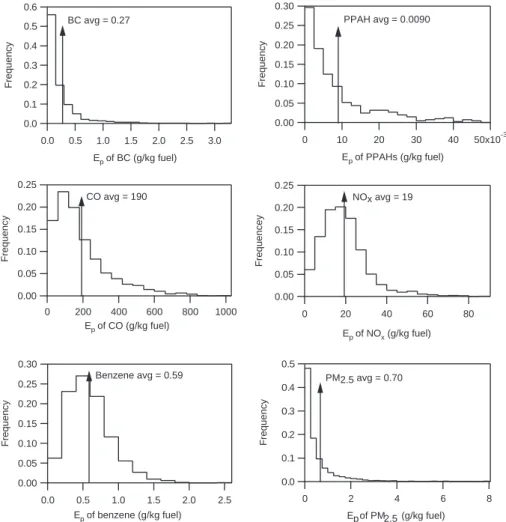
As shown in Fig. 3, the distributions of emission factors of different species are skewed to varying degrees. The distributions of those species with modes near zero, such as BC, PPAHs, and PM_2.5, are dramatically skewed by a small number of high 25

(14)

ACPD

Full Screen / Esc

EGU

skewness coefficient, a measure of the symmetry of a distribution where 0 is perfectly symmetric, of BC and PM_2.5emission factors is 5–6; and that of the other species is <2 in all cases. The few data points with very high values considerably affect the means of BC, PPAHs, CO, and PM_2.5. The implications of the different distribution patterns are discussed in the following section.

5

3.2. Emission inventory

Table 3 compares our results to the Mexican government’s official motor vehicle emis-sion inventory for the year 2002, the most recent year for which such estimates are available. For NO_x and VOCs, our estimates represent lower limits due to the instru-ments’ slower response times, as discussed previously. The Secretar´ıa del Medio 10

Ambiente y Recursos Naturales, the Mexican equivalent of the US Environmental Pro-tection Agency (EPA), has been producing inventories since 1996 using a customized version of EPA’s MOBILE model and light-duty gasoline emission factors measured by the Instituto Mexicano del Petr ´oleo. Comparison of the official inventory against independent estimates can provide a measure of uncertainty in the inventory.

15

The reasonably good agreement between the two sets of estimates adds confidence to them. As shown in Fig. 4, our estimates of Mexico City’s motor vehicle emissions in 2003 for CO, NO_x, VOCs, and PM_2.5 are 38% lower, 23% lower, 7% higher, and 26% higher, respectively, than found in the government’s official motor vehicle emission inventory for the year 2002. For reference, it is not uncommon for such estimates to 20

disagree by factors of two (200%) or more (Fine et al., 2003; Russell and Dennis, 2000), or even by factors of up to ten (Ryerson et al., 2003), so the agreement found here is relatively good. Emission inventory models such as MOBILE have underestimated VOC and CO emissions in the past (Arriaga-Colina et al., 2004; Sawyer et al., 2000), yet our results and those of another study using fuel-based methods (Schifter et al., 25

(15)

ACPD

Full Screen / Esc

EGU

4. Discussion

4.1. Emission factors

As shown in Table 2, the emission factors of CO, NO_x, and VOCs measured in this study are similar to those found in a remote sensing study in Mexico City in 2000 (Schifter et al., 2005) and in Monterrey in 1995 (Bishop et al., 1997). Our results are 5

substantially lower than found in a remote sensing study in Mexico City in 1991 (Beaton et al., 1992). Our mean CO emission factor is 23% higher than the year 2000 measure-ment. The difference may stem from the mobile lab’s ability to capture a wider range of engine loads compared to remote sensing, which is typically limited to sites with a single lane of traffic and requires uphill grades or locations with moderate accelerations 10

to capture a signal. The NO_x emission factors agree well. If the remote sensing VOC measurement is scaled upward by a factor of two, as suggested to account for varying absorptions by different VOCs (Singer et al., 1998), then the corrected value of 36 g kg−1is essentially equivalent to our estimate.

Table 2 also shows that over a 12-year period between 1991 and 2003, CO and VOC 15

emission factors fell by 60% and 83% (again applying the factor-of-two correction for the 1991 VOC measurement), respectively, if we assume that remote sensing and the mobile lab provide equivalent results. At the very least, we can assert that emission factors of these two pollutants have fallen significantly. The introduction of catalytic converters in 1991 likely played a large role in these reductions, with the effect slowly 20

propagating through the fleet as older cars were gradually replaced. With respect to total emissions, reductions in emission factors are partially offset by growth in fuel consumption over this period, such that the corresponding change in the emission inventory is not expected to be as large.

Mexico City’s emission factors are considerably higher than those measured in the 25

US. Because gasoline-powered vehicles are the predominant source of vehicular CO and VOC emissions (Sawyer et al., 2000), we focus on comparing Mexico City’s emis-sion factors of these two species to measurements of light-duty gasoline-powered

(16)

ve-ACPD

Full Screen / Esc

EGU

hicles in the US. Remote sensing measurements in Denver found a light-duty fleet-average CO emission factor of 65 g kg−1 in 1999–2000 (Pokharel et al., 2002). In the Caldecott Tunnel in the San Francisco Bay Area in 2001, light-duty CO emission fac-tors were 34–81 g kg−1 over a range of engine loads with vehicle specific powers of −5 to 18 W kg−1 (Kean et al., 2003). The emission factor of 190 g kg−1 measured in 5

Mexico City is 2.4–5.6 times higher than found in the US. The difference for VOC emis-sion factors is even larger. In 1997, light-duty VOC emisemis-sion factors of ∼3 g kg−1were measured in the Caldecott Tunnel (Kirchstetter et al., 1999b). Mexico City’s emission factor of 35 g kg−1measured in 2003 is more than 10 times higher, and the actual dis-crepancy is probably larger if the US emission factors have continued their historical 10

trend of declining between the years 1997 and 2003. A previous comparison using the mobile lab found that the ratio of formaldehyde to CO₂was seven times higher in Mexico City than in Boston (Kolb et al., 2004).

Because our NO_xemission factors represent a fleet-average that includes both light-and heavy-duty vehicles, a direct comparison to measurements in the US is not possi-15

ble. Remote sensing and tunnel studies have reported light-duty NO_x emission factors of 7 g kg−1 in the US in recent years (Harley et al., 2005; Pokharel et al., 2002). The average heavy-duty NO_x emission factor in the US is 39 g kg−1(Marr et al., 2002) and has not changed significantly over the past 20 years (Yanowitz et al., 2000). Mexico City’s combined NO_xemission factor of 19 g kg−1falls in between light- and heavy-duty 20

values found in the US.

The skewness of the emission factor distributions shown in Fig. 3 may indicate the degree to which a pollutant is mainly emitted by certain types of vehicles that make up a small fraction of the fleet. BC is expected to be emitted mainly by diesel vehicles, while the other pollutants are also emitted by gasoline-powered vehicles, which make 25

up the majority of the fleet. The distributions and their skewness may also be indicative of different driving modes.

The discrepancies between the mean and the mode of the distributions shown in Fig. 3 illustrate the large impact that a very small fraction of the vehicle fleet may have

(17)

ACPD

Full Screen / Esc

EGU

on the average emission factor. In fact, if the highest 20% of the points are eliminated, the average emission factors of BC, PPAHs, and PM_2.5 can be reduced by ∼50%, respectively, which corresponds to comparable reductions in the emission inventory. On the other hand, species like NO_x and benzene are not skewed as much by the “super polluters.” Eliminating the highest 20% of values will only result in a 24% and 5

23% reduction in their emissions, respectively. For CO, whose emission factors are moderately skewed, eliminating the highest 20% of values reduces the overall average by 36%. These distribution patterns suggest that policies focusing on a small fraction of the vehicle fleet, i.e. targeting the “super polluters,” will have the greatest effect on BC and PPAH emissions and less of an effect on NO_x and benzene (or VOCs).

10

4.2. Emission inventory

Although we can conclude that the mobile lab and government model give approxi-mately similar results, at least in comparison to previous studies, two sources of un-certainty prevent us from making stronger quantitative conclusions about the accuracy of the inventory. First, cold-start emissions are not captured in our on-road experi-15

ments and are therefore not included in our estimates. Second, using the ambient VOC/benzene ratio to estimate VOC emissions adds uncertainty, as other sources may also contribute to total VOC and benzene concentrations and may have different VOC/benzene ratios. By using measurements collected during the morning rush hour, when vehicle emissions are dominant and fresh, we have attempted to minimize un-20

certainty associated with using ambient concentration ratios. This uncertainty can be determined quantitatively in the future when a method for fast measurements of total VOCs becomes available in the mobile lab.

We also compare our estimates of the total emissions of BC and PPAHs to the results determined using an alternative approach, in which the ambient BC/CO and PPAH/CO 25

ratios are multiplied by the total CO emissions in the city (Table 3). The ratio of BC/CO measured at the supersite in Iztapalapa during the MCMA-2003 field campaign was 1.63±0.02 µg m−3 ppm−1 (r2=0.64), or 1.89±0.03×10−3g BC g−1 CO. The resulting

(18)

ACPD

Full Screen / Esc

EGU

estimate of BC emissions, shown in Table 3, is 35% higher than our fuel-based result, which is consistent with the common understanding that ambient measurements will detect BC emissions from sources besides on-road motor vehicles. Likewise, the am-bient PPAH/CO ratio was 19.5±0.2 ng m−3ppm−1(r2=0.71), or 2.27±0.03×10−5g PAH g−1 CO, but the alternative estimate is 53% lower than the result from the mobile lab. 5

We believe the difference is largely due to particle aging or coating that occurs dur-ing the transport from vehicle tailpipes to the ambient monitordur-ing site. Particle agdur-ing, through coagulation and coating by secondary aerosol, causes a large portion of the surface adsorbed PAHs to become undetectable to the photoionization aerosol sensor, which is sensitive only to PAHs on particle surfaces.

10

The advantage of the mobile lab is its ability to provide a comprehensive estimate of the vehicle fleet’s emissions, taking into consideration a variety of vehicle types under the full range of real-world driving conditions. In future work, we suggest using additional statistical analyses to identify the different types of engines associated with each exhaust plume point. Principal component analysis could be used to study the 15

expected covariance between, for example, high NO_xand high BC emissions that might be associated with diesel vehicles.

5. Conclusions

We have used a mobile lab to measure fleet-average emission factors of BC, PPAHs, and other species in Mexico City. Out of 75 h of sampling, the method has identi-20

fied ∼30 000 data points corresponding to exhaust plumes. Motor vehicles are es-timated to emit 1700±200 metric tons BC, 57±6 tons PPAHs, 1 190 000±40 000 tons CO, 120 000±3000 tons NO_x, 202 000±4000 tons VOCs, and 4400±400 tons PM_2.5per year. The estimates for CO, NO_x, and PPAHs may be low by ∼10% due to the slower response time of analyzers used to measure these species. The distributions of the 25

emission factors are skewed to varying degrees. As a result, the total emissions of BC and PPAHs can be reduced by approximately 50% if the highest 20% of data points are

(19)

ACPD

Full Screen / Esc

EGU

removed, but the “super polluters” are less influential on NO_x and VOC emissions. A fast measurement technique for total VOCs is desired in order to more directly estimate VOC emissions using this method. This method can be combined with manual analysis of chase events, so that the emissions of individual vehicles or vehicle classes can be studied while self-sampling and on-road background measurements are conveniently 5

detected and separated from those of the real exhaust plumes.

Acknowledgements. This research was supported by funds from the Alliance for Global

Sus-tainability, the Mexican Metropolitan Environmental Commission to the Integrated Program on Urban, Regional and Global Air Pollution at MIT, and the National Science Foundation. We are also grateful to Aerodyne Research Inc. and other participants in MCMA-2003 field campaign,

10

RAMA and PEMEX for providing additional data, and Robert Slott for technical advice.

References

Arriaga-Colina, J. L., West, J. J., Sosa, G., Escolona, S. S., Ordunez, R. M., and Cervantes, A. D. M.: Measurements of VOCs in Mexico City (1992–2001) and evaluation of VOCs and CO in the emissions inventory, Atmos. Environ., 38, 2523–2533, 2004.

15

Beaton, S. P., Bishop, G. A., and Stedman, D. H.: Emission characteristics of Mexico City vehicles, J. Air Waste Manage. Assoc., 42, 1424–1429, 1992.

Bishop, G. A., Stedman, D. H., Garza Castro, J., and D ´avalos, F. J.: On-road remote sensing of vehicle emissions in Mexico, Environ. Sci. Technol., 31, 3505–3510, 1997.

Bocskay, K. A., Tang, D., Orjuela, M. A., Liu, X., Warburton, D. P., and Perera, F. P.:

Chro-20

mosomal aberrations in cord blood are associated with prenatal exposure to carcinogenic polycyclic aromatic hydrocarbons, Cancer Epidemiol. Biomarkers Prevention, 14, 506–511, 2005.

Canagaratna, M. R., Jayne, J. T., Ghertner, D. A., Herndon, S., Shi, Q., Jimenez, J. L., Silva, P. J., Wiiliams, P., Lanni, T., Drewnick, F., Demerjian, K. L., Kolb, C. E., and Worsnop, D.

25

R.: Chase studies of particulate emissions from in-use New York City vehicles, Aerosol Sci. Technol., 38, 555–573, 2004.

Comisi ón Ambiental Metropolitana: Inventario de Emisiones de la Zona Metropolitana del Valle de M éxico, Secretar´ıa del Medio Ambiente, Gobierno de México, Mexico, 2004.

(20)

ACPD

Full Screen / Esc

EGU

Denissenko, M. F., Pao, A., Tang, M. S., and Pfeiffer, G. P.: Preferential formation of benzo[a]pyrene adducts at lung cancer mutational hotspots in P53, Sci., 274, 430–432, 1996.

Fine, J., Vuilleumier, L., Reynolds, S., Roth, P., and Brown, N.: Evaluating uncertainties in re-gional photochemical air quality modeling, Annu. Rev. Environ. Resour., 28, 59–106, 2003.

5

Finlayson-Pitts, B. J. and Pitts, J. N.: Chemistry of the Upper and Lower Atmosphere, Academic Press, San Diego, 2000.

Gakenheimer, R., Molina, L. T., Sussman, J., Zegras, C., Howitt, A., Makler, J., Lacy, R., Slott, R., Villegas, A., Molina, M. J., and S ´anchez, S.: The MCMA transportation system: mobility and air pollution, in: Air Quality in the Mexico Megacity, edited by: Molina, L. T. and Molina,

10

M. J., Kluwer Academic Publishers, Boston, 2002.

Gamas, E. D., Diaz, L., Rodriguez, R., L ´opez-Salinas, E., Schifter, I., and Ontiveros, L.: Ex-haust emissions from gasoline- and LPG-powered vehicles operating at the altitude of Mex-ico City, J. Air Waste Manage. Assoc., 49, 1179–1189, 1999.

Hansen, A. D. A. and Rosen, H.: Individual measurements of the emission factor of aerosol

15

black carbon in automobile plumes, J. Air Waste Manage. Assoc., 40, 1654–1657, 1990. Harley, R. A., Marr, L. C., Lehner, J. K., and Giddings, S. N.: Changes in motor vehicle

emis-sions on diurnal to decadal time scales and effects on atmospheric composition, Environ. Sci. Technol., 39, 5356–5362, 2005.

Instituto Mexicano del Petr ´oleo (IMP): Demanda de Petrol´ıferos en la ZMCM,

20

INDA/RPDA/SROYC, Registro de Derecho de Autor No. 03-2001-113012253600-01, Mexico, D.F., 2001.

Jacobson, M. Z.: Control of fossil-fuel particulate black carbon and organic matter, possibly the most effective method of slowing global warming, J. Geophys. Res., 107, art. no. 4410, doi:10.1029/2001JD001366, 2002.

25

Jimenez, J. L., McManus, J. B., Shorter, J. H., Nelson, D. D., Zahniser, M. S., Koplow, M., McRae, G. J., and Kolb, C. E.: Cross road and mobile tunable infrared laser measurements of nitrous oxide emissions from motor vehicles, Chemosphere – Global Change Science, 2, 397–412, 2000.

Kean, A. J., Harley, R. A., and Kendall, G. R.: Effects of vehicle speed and engine load on

30

motor vehicle emissions, Environ. Sci. Technol., 37, 3739–3746, 2003.

Kirchstetter, T. W., Harley, R. A., Kreisberg, N. M., Stolzenburg, M. R., and Hering, S. V.: On-road measurement of fine particle and nitrogen oxide emissions from light- and heavy-duty

(21)

ACPD

Full Screen / Esc

EGU

motor vehicles, Atmos. Environ., 33, 2955–2968, 1999a.

Kirchstetter, T. W., Singer, B. C., Harley, R. A., Kendall, G. R., and Traverse, M.: Impact of Cal-ifornia reformulated gasoline on motor vehicle emissions. 1. Mass emission rates, Environ. Sci. Technol., 33, 318–328, 1999b.

Kolb, C. E., Herndon, S. C., McManus, J. B., Shorter, J. H., Zahniser, M. S., Nelson, D. D.,

5

Jayne, J. T., Canagaratna, M. R., and Worsnop, D. R.: Mobile laboratory with rapid response instruments for real-time measurements of urban and regional trace gas and particulate distributions and emission source characteristics, Environ. Sci. Technol., 38, 5694–5703, 2004.

Lamb, B., Velasco, E., Allwine, E., Westberg, H., Herndon, S., Knighton, B., and Grimsrud,

10

E.: Ambient VOC measurements in Mexico City during the 2002 and 2003 field campaigns, The 84th AMS Annual Meeting: Sixth Conference on Atmospheric Chemistry, Seattle, WA, P1.16, 2004.

Lobscheid, A. B. and McKone, T. E.: Constraining uncertainties about the sources and magni-tude of polycyclic aromatic hydrocarbon (PAH) levels in ambient air: the state of Minnesota

15

as a case study, Atmos. Environ., 38, 5501–5515, 2004.

Marr, L. C., Black, D. R., and Harley, R. A.: Formation of photochemical air pollution in central California 1. Development of a revised motor vehicle emission inventory, J. Geophys. Res., 107, art. no. 4047, doi:10.1029/2001JD000690, 2002.

Marr, L. C., Grogan, L. A., Worhnschimmel, H., Molina, L. T., Molina, M. J., Smith, T. J., and

20

Garshick, E.: Vehicle traffic as a source of particulate polycyclic aromatic hydrocarbon expo-sure in Mexico City, Environ. Sci. Technol., 38, 2584–2592, 2004.

Marr, L. C., Kirchstetter, T. W., Harley, R. A., Miguel, A. H., Hering, S. V., and Hammond, S. K.: Characterization of polycyclic aromatic hydrocarbons in motor vehicle fuels and exhaust emissions, Environ. Sci. Technol., 33, 3091–3099, 1999.

25

Molina, L. T. and Molina, M. J.: Clearing the air: a comparative study, in Air Quality in the Mexico Megacity: An Integrated Assessment, edited by: Molina, L. T. and Molina, M. J., Kluwer Academic Publishers, Boston, 2002.

Moosm ¨uller, H., Arnott, W. P., Rogers, C. F., Bowen, J. L., Gillies, J. A., Pierson, W. R., Collins, J. F., Durbin, T. D., and Norbeck, J. M.: Time resolved characterization of diesel particulate

30

emissions. 1. Instruments for particle mass measurements, Environ. Sci. Technol., 35, 781– 787, 2001.

(22)

in-ACPD

Full Screen / Esc

EGU

ventory for Denver: an efficient alternative to modeling, Atmos. Environ., 36, 5177–5184, 2002.

Russell, A. and Dennis, R.: NARSTO critical review of photochemical models and modeling, Atmos. Environ., 34, 2283–2324, 2000.

Ryerson, T. B., Trainer, M., Angevine, W. M., Brock, C. A., Dissly, R. W., Fehsenfeld, F. C., Frost,

5

G. J., Goldan, P. D., Holloway, J. S., Hubler, G., Jakoubek, R. O., Kuster, W. C., Neuman, J. A., Nicks Jr., D. K., Parrish, D. D., Roberts, J. M., and Sueper, D. T.: Effect of petrochem-ical industrial emissions of reactive alkenes and NO_x on tropospheric ozone formation in Houston, Texas, J. Geophys. Res., 108, art. no. 4249, doi:10.1029/2002JD003070, 2003. Sawyer, R. F., Harley, R. A., Cadle, S. H., Norbeck, J. M., Slott, R., and Bravo, H. A.: Mobile

10

sources critical review: 1998 NARSTO assessment, Atmos. Environ., 34, 2161–2181, 2000. Schifter, I., D´ıaz, L., M´ugica, V., and L´opez-Salinas, E.: Fuel-based motor vehicle emission

inventory for the metropolitan area of Mexico city, Atmos. Environ., 39, 931–940, 2005. Schifter, I., D´ıaz, L., Vera, M., Castillo, M., Ramos, F., Avalos, S., and Lopez-Salinas, E.: Impact

of engine technology on the vehicular emissions of Mexico City, Environ. Sci. Technol., 34,

15

2663–2667, 2000.

Singer, B. C., Harley, R. A., Littlejohn, D., Ho, J., and Vo, T.: Scaling of infrared remote sensor hydrocarbon measurements for motor vehicle emission inventory calculations, Environ. Sci. Technol., 32, 3241–3248, 1998.

Singer, B. C. and Harley, R. A.: A fuel-based inventory of motor vehicle exhaust emissions in

20

the Los Angeles area during summer 1997, Atmos. Environ., 34, 1783–1795, 2000.

Waggoner, A. P., Weiss, R. E., Ahlquist, N. C., Covert, D. S., Will, S., and Charlson, R. J.: Optical characteristics of atmospheric aerosols, Atmos. Environ., 15, 1891–1909, 1981. Weingartner, E., Keller, C., Stahel, W. A., Burtscher, H., and Baltensperger, U.: Aerosol

emis-sion in a road tunnel, Atmos. Environ., 31, 451–462, 1997.

25

Yanowitz, J., McCormick, R. L., and Grabowski, M. S.: In-use emissions from heavy-duty diesel vehicles, Environ. Sci. Technol., 34, 729–740, 2000.

(23)

ACPD

Full Screen / Esc

EGU

Table 1. Comparison of Mexico City BC and PPAH emission factors to those measured

else-where.

Location Method BC (g kg−1) PPAHs (g kg−1)

Mexico City 2003 Mobile lab 0.27±0.59 0.01±0.01a

Los Angeles, CA 1985b Remote sensing 0.0034–0.85 N/Ac

Zurich, Switzerland 1993d Tunnel study LDV: 0.02

HDV: 0.3

LDV: 0.002 HDV: 0.007

Oakland, CA 1997e Tunnel study LDV: 0.035±0.003

HDV: 1.3±0.3

LDV: 9.0×10−5 HDV: 0.0023

a

Values reported for species measured by analyzers with slower response times may be un-derestimated by up to 10%, as discussed in the text.

b

Range reported for measurements of individual vehicles (Hansen and Rosen, 1990).

c

Not available.

d

Results reported separately for light-duty vehicles (LDV) and heavy-duty vehicles (HDV). Re-sults originally reported in units of mg km−1 (Weingartner et al., 1997). We assumed a fuel economy of 10 km L−1for LDVs and 2 km L−1 for HDVs to convert to fuel-based emission fac-tors.

e

The PAH emission factor is the sum of 10 individual species (Kirchstetter et al., 1999a; Marr et al., 1999)

(24)

ACPD

Full Screen / Esc

EGU

Table 2. Fuel-based emission factors (g kg−1) from on-road motor vehicles measured in this study and in remote sensing studies in Mexico.

(g kg−1) Vehicle types CO Benzene VOC NOa_x PM_2.5

Mexico City 2003b all 190±160c 0.60±0.32 32±17 19±12c 0.7±1.4d

Mexico City 2000e light-duty 155±18 N/Af 18±3g 21±5 N/A

Monterrey 1995h light-duty 205±23 N/A 12±3g 30±8 N/A

Mexico City 1991i light-duty 475±200 N/A 96±29g N/A N/A

a

NO_xis reported as NO₂.

b

Mean and standard deviation across all individual measurements.

c

d

This estimate does not include the additional uncertainty imposed by the limitations of the PM_2.5measurement method, as discussed in the text.

e

A remote sensing study that reports the mean and 95% confidence intervals across 12 site means (Schifter et al., 2005).

f

Not available.

g

Hydrocarbons only. These values do not include the factor-of-two correction to account for varying absorption by different species (Singer, 2000).

h

A remote sensing study that reports the mean and standard deviation across four site means (Bishop et al., 1997).

i

A remote sensing study that reports the mean and standard deviation across nine days of sampling at five locations (Beaton et al., 1992).

(25)

ACPD

Full Screen / Esc

EGU

Table 3. Comparison of the motor vehicle emission inventory in Mexico City.

Pollutant

(metric tons yr−1)

This studya Official inventory or alternative approach

BC 1700±200 2300±100c PPAHs 57±6b 27±1c CO 1 190 000±40 000b 1 927 101 NOd_x 120 000±3000b 156 311 VOC 202 000±4000 188 530 PM_2.5 4400±400e 3518 a

Range shows 95% confidence interval, and results from this study do not include cold starts.

b

c

The government produces estimates of CO, VOC, NO_x, and PM_2.5emissions (Comisi ´on Am-biental Metropolitana, 2004) but does not estimate emissions of BC or PPAH. To develop alternative estimates for these species, we multiplied the ambient ratios ∆[BC]/∆[CO] and ∆[PPAH]/∆[CO] measured during the field campaign, by our estimate of total CO emissions.

d

Reported as NO₂.

e

This estimate does not include the additional uncertainty imposed by the limitations of the PM_2.5measurement method, as discussed in the text.

(26)

ACPD

Full Screen / Esc

EGU

Figure 1. Schematic of the ARI mobile lab as instrumented for the MCMA-2003 field campaign.

23

Fig. 1. Schematic of the Aerodyne mobile lab as instrumented for the MCMA-2003 field

cam-paign.

(27)

ACPD

Full Screen / Esc

Print Version Interactive Discussion EGU 1200 1000 800 600 400 CO 2 (ppm) 8:30 AM 8:45 AM 9:00 AM 9:15 AM driving parked CO₂ Baseline Plume threshold

Fig. 2. CO₂concentrations measured by the mobile lab on 1 May 2003. The van was parked at the supersite until 8:52 a.m., at which time it began driving. Data points above the plume threshold (42 ppm above baseline) during the driving period are considered potential exhaust plumes.

(28)

ACPD

Full Screen / Esc

Print Version Interactive Discussion EGU 0.5 0.4 0.3 0.2 0.1 0.0 Frequency 8 6 4 2 0 Ep of PM2.5 (g/kg fuel) PM2.5 avg = 0.70 0.6 0.5 0.4 0.3 0.2 0.1 0.0 Frequency 3.0 2.5 2.0 1.5 1.0 0.5 0.0 Ep of BC (g/kg fuel) BC avg = 0.27 0.30 0.25 0.20 0.15 0.10 0.05 0.00 Frequency 50x10-3 40 30 20 10 0 Ep of PPAHs (g/kg fuel) PPAH avg = 0.0090 0.25 0.20 0.15 0.10 0.05 0.00 Frequency 1000 800 600 400 200 0 Ep of CO (g/kg fuel) CO avg = 190 0.30 0.25 0.20 0.15 0.10 0.05 0.00 Frequency 2.5 2.0 1.5 1.0 0.5 0.0 E_p of benzene (g/kg fuel) Benzene avg = 0.59 0.25 0.20 0.15 0.10 0.05 0.00 Frequencey 80 60 40 20 0 Ep of NOx (g/kg fuel) NOx avg = 19

Fig. 3. Normalized distributions and averages of emission factors of BC, PPAH, CO, NO_x, benzene, and PM_2.5. Note that the range of the y-axis varies.

(29)

ACPD

Full Screen / Esc

Print Version Interactive Discussion EGU 250x103 200 150 100 50 0 Emissions (tons yr -1 ) CO/10 NO_x VOC PM_2.5*10 * * *

Official 2002 This study 2003

Fig. 4. Motor vehicle emissions (metric tons per year) of CO, NO_x, VOCs, and PM_2.5in the Mex-ico City Metropolitan Area: the government’s official inventory for the year 2002 (all emissions) and estimates using the mobile lab fuel-based method for the year 2003 (not including cold starts). Error bars show the 95% confidence intervals. The mobile lab estimates of CO, NO_x, and PM_2.5emissions are subject to additional measurement uncertainties (*), as described in the text.